Hiding columns in excel - Word и Excel - помощь в работе с программами

Hide or show rows or columns

Hide or unhide columns in your spreadsheet to show just the data that you need to see or print.

Hide columns

Select one or more columns, and then press Ctrl to select additional columns that aren’t adjacent.
Right-click the selected columns, and then select Hide.

Note: The double line between two columns is an indicator that you’ve hidden a column.

Unhide columns

Select the adjacent columns for the hidden columns.
Right-click the selected columns, and then select Unhide.

Or double-click the double line between the two columns where hidden columns exist.

Need more help?

You can always ask an expert in the Excel Tech Community or get support in the Answers community.

Hiding Excel Column(s)

Hiding a column in excel implies making it invisible so that it is removed from display. A hidden column is not deleted from the worksheet. This means that it does exist and has been only temporarily held from view. In Excel, one can hide both contiguous and non-contiguous columns. However, to use a hidden column again, it needs to be unhidden at first.

For example, a column containing calculations may be hidden. This helps avoid confusion amongst users of a shared worksheet.

A column is hidden when its data needs to be concealed from other Excel users, it is unused and not required for a while, its presence is making comparisons between the remaining columns difficult, and so on. The purpose of hiding an excel column is to allow viewing the relevant areas of a worksheet at a given time.

Hiding Excel Column(s)
- How to Hide Columns in Excel? (Top 4 Methods)
  - Example #1–Hide Columns Using the “Hide” Option of the Context Menu
  - Example #2–Hide Excel Columns Using the “Ctrl+Zero (0)” Shortcut
  - Example #3–Hide Excel Columns by Setting the Column Width as Zero
  - Example #4–Hide Columns Using VBA Code
- Frequently Asked Questions
- Recommended Articles

How to Hide Columns in Excel? (Top 4 Methods)

The techniques of hiding columns in Excel are listed as follows:

“Hide” option of the context menu
“Ctrl+zero (0)” shortcut
Column width as zero
VBA code

Let us discuss these methods one by one with the help of examples.

Note: All the following examples demonstrate the process of hiding adjacent (contiguous) columns. For hiding multiple non-adjacent columns, refer to the second question under the heading “frequently asked questions.” This is given at the end of this article.

Example #1–Hide Columns Using the “Hide” Option of the Context Menu

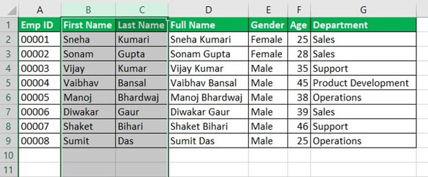
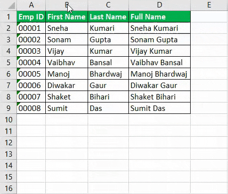
The following table displays the IDs, names, gender, age, and department of some employees of an organization. Consider one column of the table as one column of an Excel worksheet. So, the dataset begins from column A (emp ID) and ends with column G (department).

The first name (column B) and last name (column C) have been concatenated (joined) to form the full name (column D). Since columns B and C are not required (for some time), we want to hide them using the “hide” option of the context menu.

Emp ID	First Name	Last Name	Full Name	Gender	Age	Department
00001	Sneha	Kumari	Sneha Kumari	Female	25	Sales
00002	Sonam	Gupta	Sonam Gupta	Female	28	Sales
00003	Vijay	Kumar	Vijay Kumar	Male	35	Support
00004	Vaibhav	Bansal	Vaibhav Bansal	Male	45	Product Development
00005	Manoj	Bhardwaj	Manoj Bhardwaj	Male	38	Operations
00006	Diwakar	Gaur	Diwakar Gaur	Male	39	Sales
00007	Shaket	Bihari	Shaket Bihari	Male	46	Support
00008	Sumit	Das	Sumit Das	Male	25	Operations

The steps to hide excel columns is listed as follows:

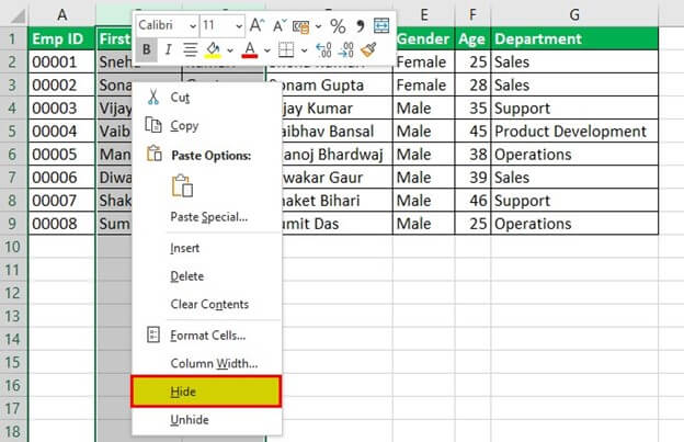
With the help of the mouse, click the label of column B appearing on top. This selects column B entirely. Next, press the keys “Shift+right arrow” to select the entire column C.
The selection is shown in the succeeding image. Notice that in column A, the numbers have been formatted as text. This has been done to place zeros before each number in cells A2 to A9.

Note 1: For “Shift+right arrow” to work, hold the “Shift” key, and at the same time, press the right arrow. When the shortcut “Shift+right arrow” is pressed after selecting a column, the selection is extended to an adjacent column on the right.

When the shortcut “Shift+right arrow” is pressed after selecting a cell, the selection is extended to an adjacent cell on the right.

Note 2: When the numbers of column A were formatted as text, green triangles (shown in the first image of example #2) had appeared on the upper-left corner of each cell. From the “trace error” button, we clicked “ignore error” (for each cell) to remove such green triangles.
Right-click the selection and choose “hide” from the context menu. The same is shown in the following image.
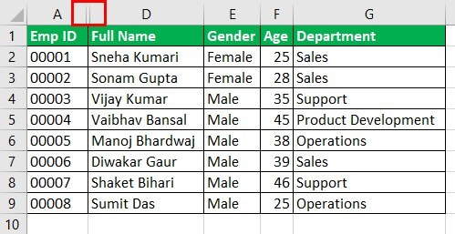
The final dataset, with columns B and C hidden, is shown in the following image. Notice that there are double vertical lines (shown in a red box) between the column labels A and D. These lines indicate that columns B and C have been hidden.

Another indication of hidden excel columns is the change in the sequence of the column labels. After label A, labels B and C are skipped, and straightaway label D is displayed.

Example #2–Hide Excel Columns Using the “Ctrl+Zero (0)” Shortcut

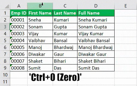
The following image shows a dataset similar to that of example #1. Notice that the number of columns has been reduced this time. Columns A to D are displayed, which consist of the employee ID, first name, last name, and full name respectively.

Ignore the green triangles in column A of the subsequent images. These are displayed because the “ignore error” option from the “trace error” button has not been clicked, unlike in step 1 of the preceding example (example #1).

We want to hide columns B and C by using the shortcut “Ctrl+zero (0)” in Excel.

The steps to hide the stated columns using the given technique are listed as follows:

Step 1: Select columns B and C, which need to be hidden. For this, click the label of column B with the mouse and drag it across to column C. When the mouse pointer is placed on the label of column B, it changes to an arrow pointing downwards.

Note: Alternatively, select any cell of column B and press the keys “Ctrl+space” together. Column B is selected entirely. Next, press the keys “Shift+right arrow” to select column C.

Step 2: Once the columns to be hidden (columns B and C) are selected, press the keys “Ctrl+zero (0)” together.

The steps 1 and 2 are shown in the following image. Hence, columns B and C (selected in step 1) are hidden. Notice that, in the final output, the double vertical lines separate the labels of columns A and D.

Example #3–Hide Excel Columns by Setting the Column Width as Zero

Working on the dataset of example #2, we want to hide columns B and C by setting the column widthA user can set the width of a column in an excel worksheet between 0 and 255, where one character width equals one unit. The column width for a new excel sheet is 8.43 characters, which is equal to 64 pixels.read more as zero.

The steps to hide the mentioned columns using the given technique are listed as follows:

Step 1: Select the columns to be hidden. So, select columns B and C entirely.

Step 2: Right-click the selection and choose “column width” from the context menu. Set column width as zero and click “Ok.”

Both steps 1 and 2 are shown in the following image. The final dataset, with columns B and C hidden, is also displayed in this image. Double vertical lines appear between the labels of columns A and D.

Note: When a column’s width is entered as zero, the column is hidden from the worksheet.

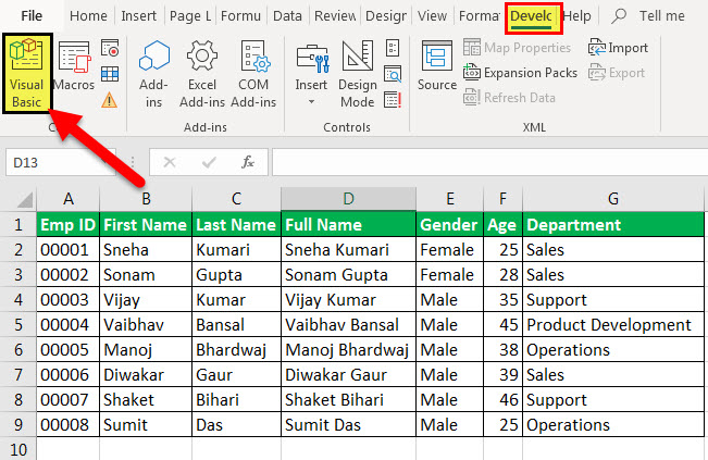
Example #4–Hide Columns Using VBA Code

Working on the dataset of example #1, we want to hide columns B and C with the help of a VBA codeVBA code refers to a set of instructions written by the user in the Visual Basic Applications programming language on a Visual Basic Editor (VBE) to perform a specific task.read more. Consider the dataset to be in “sheet1” of Excel.

The steps to hide columns using a VBA code are listed as follows:

Step 1: From the Developer tab, click “visual basic.” This is shown in the following image.

Note: If the Developer tabEnabling the developer tab in excel can help the user perform various functions for VBA, Macros and Add-ins like importing and exporting XML, designing forms, etc. This tab is disabled by default on excel; thus, the user needs to enable it first from the options menu.read more is not displayed on the ribbon, it must be enabled from the File tab. For the detailed steps, click the given hyperlink.

Step 2: A new window titled “Microsoft visual basic for applications” opens. Double-click “sheet1.” Next, from the Insert tab, click “procedure.” Specify the name of the procedure and paste the following code:

Worksheets(“Sheet1”).Columns(“B:C”).Hidden = True

This is shown in the following image.

Step 3: Save the file with the .xlsm extension as it supports macros. This extension is used for a macro-enabled workbook, which has been created in Excel 2007 or the newer Excel versions.

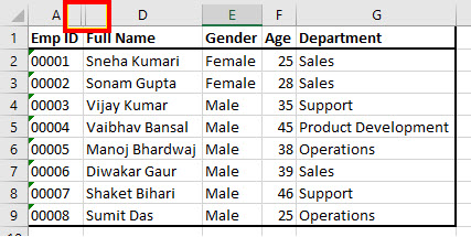
Step 4: From the Run tab, click “run sub/user form.” The output is shown in the following image. Notice the double line (shown in a red box) between the column labels A and D. This indicates that the columns in between (i.e., columns B and C) are hidden.

Frequently Asked Questions

1. What does it mean to hide columns and how is it done in Excel?

To hide a column means removing one or more excel columns from the display. Such hidden columns do exist in the worksheet even though they become invisible. Columns are usually hidden when they are neither being used nor meant to be deleted.

The steps to hide a column in Excel are listed as follows:

a. Select the column to be hidden.
b. Right-click the selection and choose “hide” from the context menu.

The column selected in step “a” is hidden.

Note: For more techniques of hiding a column, refer to the examples of this article.

2. How to hide multiple columns in Excel?

The steps to hide multiple columns in Excel are listed as follows:

a. Select all the columns that need to be hidden.
• For selecting multiple contiguous columns, drag across the column labels with the mouse. Alternatively, select the first column and press the keys “Shift+right arrow” to select columns on the right.
• For selecting multiple non-contiguous columns, click the first column label. Thereafter, hold the “Ctrl” key and click the other column labels.
b. From the Home tab, click the “format” drop-down in the “cells” group.
c. Under “visibility,” select “hide & unhide.” Next, choose “hide columns.”

The columns selected in step “a” are hidden.

3. How to hide and lock columns in Excel?

The steps to hide and lock columns in Excel are listed as follows:

a. Select the entire worksheet by pressing either the keys “Ctrl+A” or the “select all” button. The “select all” button is located at the top-left corner of the Excel worksheet.
b. Right-click the selection and choose “format cells” from the context menu. The “format cells” dialog box opens. Uncheck the “locked” option in the “protection” tab. Click “Ok.”
c. Select the columns to be hidden and locked. Open the “format cells” dialog box again and click the “protection” tab. Check the “locked” option and click “Ok.”
d. Hide the columns selected in the preceding step (step c). For this, keep the columns to be hidden selected and click the “format” drop-down from the Home tab. Next, click “hide columns” from the “hide & unhide” option.
e. From the Review tab, click “protect sheet.” The “protect sheet” dialog box opens. Keep the following checkboxes selected:
• “Protect worksheet and contents of locked cell”
• “Select locked cells”
• “Select unlocked cells”
f. Enter a password and confirm it. Click “Ok” to proceed. The “protect sheet” dialog box closes.

The columns selected in step “c” are hidden. Since the worksheet is protected, these hidden columns cannot be unhidden by the usual ways to unhide a column. The advantage of locking hidden columns is that their content is concealed from the other users of the worksheet.

Note: To unhide the hidden columns, unprotect the sheet in the first place. To unprotect the sheet, click “unprotect sheet” from the Review tab. Next, enter the password and click “Ok.”

Thereafter, unhide the columns by selecting, right-clicking, and choosing “unhide” from the context menu. Alternatively, select the columns and choose “unhide columns” from the “hide & unhide” option of the “format” drop-down (in the Home tab).

Steps

1
Double-click your spreadsheet to open it in Excel.
- If Excel is already open, you can open your spreadsheet by pressing Ctrl + O (Windows) or Cmd + O (macOS) and then selecting the file.
2
Click the letter above the column you want to hide. This selects the entire column.
- For example, to select the first column (column A), click the A at the top of the column.
- If you want to hide multiple columns at once, just click and drag your cursor over the column letters you want to hide.
- You can also select multiple non-adjacent columns by holding down Ctrl as you click each column letter.
Advertisement
3
Right-click the selected column(s). This brings up a menu.
- If you don’t have multiple mouse buttons, hold down the Ctrl key as you click the column(s) instead.
4

Click Hide on the menu. Any selected columns are now hidden.^[1]
5

Unhide columns (optional). If you want to show columns that are hidden, just click any column adjacent to those hidden to select it, and then choose Unhide.

Ask a Question

200 characters left

Include your email address to get a message when this question is answered.

Submit

Thanks for submitting a tip for review!

References

About This Article

Article SummaryX

1. Open your spreadsheet.
2. Select the column(s) you want to hide.

3. Right-click the selected column(s).
4. Click Hide.

Did this summary help you?

Thanks to all authors for creating a page that has been read 42,783 times.

Is this article up to date?

Источник

Hide | Unhide | Multiple Columns or Rows | Hidden Tricks

Sometimes it can be useful to hide columns or rows in Excel.

Hide

To hide a column, execute the following steps.

1. Select a column.

2. Right click, and then click Hide.

Result:

Note: to hide a row, select a row, right click, and then click Hide.

Unhide

To unhide a column, execute the following steps.

1. Select the columns on either side of the hidden column.

2. Right click, and then click Unhide.

Result:

Note: to unhide a row, select the rows on either side of the hidden row, right click, and then click Unhide.

Multiple Columns or Rows

To hide multiple columns, execute the following steps.

1. Select multiple columns by clicking and dragging over the column headers.

2. To select non-adjacent columns, hold CTRL while clicking the column headers.

3. Right click, and then click Hide.

Result:

To unhide all columns, execute the following steps.

4. Select all columns by clicking the Select All button.

5. Right click a column header, and then click Unhide.

Result:

Note: in a similar way, you can hide and unhide multiple rows.

Hidden Tricks

Impress your boss with the following hidden tricks. To hide and show columns with the click of a button, execute the following steps.

1. Select one or more columns.

2. On the Data tab, in the Outline group, click Group.

3. To hide the columns, click the minus sign.

4. To show the columns again, click the plus sign.

Note: to ungroup the columns, first, select the columns. Next, on the Data tab, in the Outline group, click Ungroup.

Finally, to hide cells in Excel, execute the following steps.

1. Select a range of cells.

2. Right click, and then click Format Cells.

The ‘Format Cells’ dialog box appears.

3. Select Custom.

4. Type the following number format code: ;;;

5. Click OK.

Result:

Note: the data is still there. Try it yourself. Download the Excel file, hide cells, select one of the hidden cells and look at the formula bar.

Источник

Learn several ways to do this

Updated on September 19, 2022

What to Know

Hide a column: Select a cell in the column to hide, then press Ctrl+0. To unhide, select an adjacent column and press Ctrl+Shift+0.
Hide a row: Select a cell in the row you want to hide, then press Ctrl+9. To unhide, select an adjacent column and press Ctrl+Shift+9.
You can also use the right-click context menu and the format options on the Home tab to hide or unhide individual rows and columns.

You can hide columns and rows in Excel to make a cleaner worksheet without deleting data you might need later, although there is no way to hide individual cells. In this guide, we provide instructions for three ways to hide and unhide columns in Excel 2019, 2016, 2013, 2010, 2007, and Excel for Microsoft 365.

Hide Columns in Excel Using a Keyboard Shortcut

The keyboard key combination for hiding columns is Ctrl+0.

Click on a cell in the column you want to hide to make it the active cell.
Press and hold down the Ctrl key on the keyboard.
Press and release the 0 key without releasing the Ctrl key. The column containing the active cell should be hidden from view.

To hide multiple columns using the keyboard shortcut, highlight at least one cell in each column to be hidden, and then repeat steps two and three above.

Hide Columns Using the Context Menu

The options available in the context — or right-click menu — change depending upon the object selected when you open the menu. If the Hide option, as shown in the image below, is not available in the context menu it is likely that you didn’t select the entire column before right-clicking.

Hide a Single Column
Click the column header of the column you want to hide to select the entire column.
Right-click on the selected column to open the context menu.
Choose Hide. The selected column, the column letter, and any data in the column will be hidden from view.

Hide Adjacent Columns
In the column header, click and drag with the mouse pointer to highlight all three columns.
Right-click on the selected columns.
Choose Hide. The selected columns and column letters will be hidden from view.

When you hide columns and rows containing data, it does not delete the data, and you can still reference it in formulas and charts. Hidden formulas containing cell references will update if the data in the referenced cells changes.

Hide Separated Columns

In the column header click on the first column to be hidden.
Press and hold down the Ctrl key on the keyboard.
Continue to hold down the Ctrl key and click once on each additional column to be hidden to select them.
Release the Ctrl key.
In the column header, right-click on one of the selected columns and choose Hide. The selected columns and column letters will be hidden from view.

When hiding separate columns, if the mouse pointer is not over the column header when you click the right mouse button, the hide option will not be available.

Hide and Unhide Columns in Excel Using the Name Box

This method can be used to unhide any single column. In our example, we will be using column A.

Type the cell reference A1 into the Name Box.
Press the Enter key on the keyboard to select the hidden column.
Click on the Home tab of the ribbon.
Click on the Format icon on the ribbon to open the drop-down.
In the Visibility section of the menu, choose Hide & Unhide > Hide Columns or Unhide Column.

Unhide Columns Using a Keyboard Shortcut

The key combination for unhiding columns is Ctrl+Shift+0.

Type the cell reference A1 into the Name Box.
Press the Enter key on the keyboard to select the hidden column.
Press and hold down the Ctrl and the Shift keys on the keyboard.
Press and release the 0 key without releasing the Ctrl and Shift keys.

To unhide one or more columns, highlight at least one cell in the columns on either side of the hidden column(s) with the mouse pointer.

Click and drag with the mouse to highlight columns A to G.
Press and hold down the Ctrl and the Shift keys on the keyboard.
Press and release the 0 key without releasing the Ctrl and Shift keys. The hidden column(s) will become visible.

The Ctrl+Shift+0 keyboard shortcut might not work depending on the version of Windows you’re running, for reasons not explained by Microsoft. If this shortcut doesn’t work, use another method from the article.

Unhide Columns Using the Context Menu

As with the shortcut key method above, you must select at least one column on either side of a hidden column or columns to unhide them. For example, to unhide columns D, E, and G:
Hover the mouse pointer over column C in the column header. Click and drag with the mouse to highlight columns C to H to unhide all columns at one time.
Right-click on the selected columns and choose Unhide. The hidden column(s) will become visible.

Hide Rows Using Shortcut Keys

The keyboard key combination for hiding rows is Ctrl+9:

Click on a cell in the row you want to hide to make it the active cell.
Press and hold down the Ctrl key on the keyboard.
Press and release the 9 key without releasing the Ctrl key. The row containing the active cell should be hidden from view.

To hide multiple rows using the keyboard shortcut, highlight at least one cell in each row you want to hide, and then repeat steps two and three above.

Hide Rows Using the Context Menu

The options available in the context menu — or right-click — change depending upon the object selected when you open it. If the Hide option, as shown in the image above, is not available in the context menu it is because you probably didn’t select the entire row.

Hide a Single Row

Click on the row header for the row to be hidden to select the entire row.
Right-click on the selected row to open the context menu.
Choose Hide. The selected row, the row letter, and any data in the row will be hidden from view.

Hide Adjacent Rows

In the row header, click and drag with the mouse pointer to highlight all three rows.
Right-click on the selected rows and choose Hide. The selected rows will be hidden from view.

Hide Separated Rows

In the row header, click on the first row to be hidden.
Press and hold down the Ctrl key on the keyboard.
Continue to hold down the Ctrl key and click once on each additional row to be hidden to select them.
Right-click on one of the selected rows and choose Hide. The selected rows will be hidden from view.

Hide and Unhide Rows Using the Name Box

This method can be used to unhide any single row. In our example, we will be using row 1.

Type the cell reference A1 into the Name Box.
Press the Enter key on the keyboard to select the hidden row.
Click on the Home tab of the ribbon.
Click on the Format icon on the ribbon to open the drop-down menu.
In the Visibility section of the menu, choose Hide & Unhide > Hide Rows or Unhide Row.

Unhide Rows Using a Keyboard Shortcut

The key combination for unhiding rows is Ctrl+Shift+9.

Unhide Rows using Shortcut Keys and Name Box

Type the cell reference A1 into the Name Box.
Press the Enter key on the keyboard to select the hidden row.
Press and hold down the Ctrl and the Shift keys on the keyboard.
Press and hold down the Ctrl and the Shift keys on the keyboard. Row 1 will become visible.

Unhide Rows Using a Keyboard Shortcut

To unhide one or more rows, highlight at least one cell in the rows on either side of the hidden row(s) with the mouse pointer. For example, you want to unhide rows 2, 4, and 6.

To unhide all rows, click and drag with the mouse to highlight rows 1 to 7.
Press and hold down the Ctrl and the Shift keys on the keyboard.
Press and release the number 9 key without releasing the Ctrl and Shift keys. The hidden row(s) will become visible.

Unhide Rows Using the Context Menu

As with the shortcut key method above, you must select at least one row on either side of a hidden row or rows to unhide them. For example, to unhide rows 3, 4, and 6:

Hover the mouse pointer over row 2 in the row header.
Click and drag with the mouse to highlight rows 2 to 7 to unhide all rows at one time.
Right-click on the selected rows and choose Unhide. The hidden row(s) will become visible.

How to Move Columns in Excel

FAQ

How do I hide cells in Excel?

Select the cell or cells you want to hide, then select the Home tab > Cells > Format > Format Cells. In the Format Cells menu, select the Number tab > Custom (under Category) and type ;;; (three semicolons), then select OK.
How do I hide gridlines in Excel?

Select the Page Layout tab, then turn off the View checkbox under Gridlines.
How do I hide formulas in Excel?

Select the cells with formulas you want to hide > select the Hidden checkbox on the Protection tab > OK > Review > Protect Sheet. Next, verify that Protect worksheet and contents of locked cells is turned on, then select OK.

Thanks for letting us know!

Get the Latest Tech News Delivered Every Day

Источник

Hide columns

Unhide columns

Need more help?

See Also

Need more help?

Hiding Excel Column(s)

Table of contents

How to Hide Columns in Excel? (Top 4 Methods)

Example #1–Hide Columns Using the “Hide” Option of the Context Menu

Example #2–Hide Excel Columns Using the “Ctrl+Zero (0)” Shortcut

Example #3–Hide Excel Columns by Setting the Column Width as Zero

Example #4–Hide Columns Using VBA Code

Frequently Asked Questions

Recommended Articles

Steps

References

About This Article

Is this article up to date?

Hide

Unhide

Multiple Columns or Rows

Hidden Tricks

What to Know

Hide Columns in Excel Using a Keyboard Shortcut

Hide Columns Using the Context Menu

Hide a Single Column

Hide Adjacent Columns

Hide Separated Columns

Hide and Unhide Columns in Excel Using the Name Box

Unhide Columns Using a Keyboard Shortcut

Unhide Columns Using the Context Menu

Hide Rows Using Shortcut Keys

Hide Rows Using the Context Menu

Hide a Single Row

Hide Adjacent Rows

Hide Separated Rows

Hide and Unhide Rows Using the Name Box

Unhide Rows Using a Keyboard Shortcut

Unhide Rows using Shortcut Keys and Name Box

Unhide Rows Using a Keyboard Shortcut

Unhide Rows Using the Context Menu