
Show or hide gridlines on a worksheet
Excel for Microsoft 365 Excel for Microsoft 365 for Mac Excel for the web Excel 2021 Excel 2021 for Mac Excel 2019 Excel 2019 for Mac Excel 2016 Excel 2016 for Mac Excel 2013 Excel 2010 Excel 2007 Excel for Mac 2011 Excel Starter 2010 More…Less
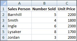
Gridlines are the faint lines that appear between cells on a worksheet.
When working with gridlines, consider the following:
-
By default, gridlines are displayed in worksheets using a color that is assigned by Excel. If you want, you can change the color of the gridlines for a particular worksheet by clicking Gridline color under Display options for this worksheet (File tab, Options, Advanced category).
-
People often confuse borders and gridlines in Excel. Gridlines cannot be customized in the same manner that borders can. If you want to change the width or other attributes of the lines for a border, see Apply or remove cell borders on a worksheet.
-
If you apply a fill color to cells on your worksheet, you won’t be able to see or print the cell gridlines for those cells. To see or print the gridlines for these cells, remove the fill color by selecting the cells, and then click the arrow next to Fill Color
 (Home tab, Font group), and To remove the fill color, click No Fill.
Note: You must remove the fill completely. If you change the fill color to white, the gridlines will remain hidden. To keep the fill color and still see lines that serve to separate cells, you can use borders instead of gridlines. For more information, see Apply or remove cell borders on a worksheet.
-
Gridlines are always applied to the whole worksheet or workbook, and can’t be applied to specific cells or ranges. If you want to apply lines selectively around specific cells or ranges of cells, you should use borders instead of, or in addition to, gridlines. For more information, see Apply or remove cell borders on a worksheet.
 (Home tab, Font group), and To remove the fill color, click No Fill.
If the design of your workbook requires it, you can hide the gridlines:
-
Select one or more worksheets.
Tip: When multiple worksheets are selected, [Group] appears in the title bar at the top of the worksheet. To cancel a selection of multiple worksheets in a workbook, click any unselected worksheet. If no unselected sheet is visible, right-click the tab of a selected sheet, and then click Ungroup Sheets.
-
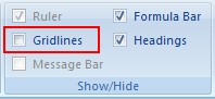
In Excel 2007: On the View tab, in the Show/Hide group, clear the Gridlines check box.
In all other Excel versions: On the View tab, in the Show group, clear the Gridlines check box.
If the gridlines on your worksheet are hidden, you can follow these steps to show them again.
-
Select one or more worksheets.
Tip: When multiple worksheets are selected, [Group] appears in the title bar at the top of the worksheet. To cancel a selection of multiple worksheets in a workbook, click any unselected worksheet. If no unselected sheet is visible, right-click the tab of a selected sheet, and then click Ungroup Sheets.
-
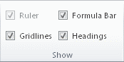
Excel 2007: On the View tab, in the Show/Hide group, select the Gridlines check box.
All other Excel versions: On the View tab, in the Show group, select the Gridlines check box.
Note: Gridlines do not print by default. For gridlines to appear on the printed page, select the Print check box under Gridlines (Page Layout tab, Sheet Options group).
-
Select the worksheet.
-
Click the Page Layout tab.
-
To show gridlines: Under Gridlines, select the View check box.
To hide gridlines: Under Gridlines, clear the View check box.
Follow these steps to show or hide gridlines.
-
Click the sheet.
-
To show gridlines: On the Layout tab, under View, select the Gridlines check box.
Note: Gridlines cannot be customized. To change the width, color, or other attributes of the lines around cells, use border formatting.
To hide gridlines: On the Layout tab, under View, clear the Gridlines check box.
Gridlines are used to distinguish cells on a worksheet. When working with gridlines, consider the following:
-
By default, gridlines are displayed on worksheets using a color that is assigned by Excel. If you want, you can change the color of the gridlines for a particular worksheet.
-
People often confuse borders and gridlines in Excel. Gridlines cannot be customized in the same way that borders can.
-
If you apply a fill color to cells on a worksheet, you won’t be able to see or print the cell gridlines for those cells. To see or print the gridlines for these cells, you must remove the fill color. Keep in mind that you must remove the fill entirely. If you simply change the fill color to white, the gridlines will remain hidden. To retain the fill color and still see lines that serve to separate cells, you can use borders instead of gridlines.
-
Gridlines are always applied to the entire worksheet or workbook and can’t be applied to specific cells or ranges. If you want to selectively apply lines around specific cells or ranges of cells, you should use borders instead of, or in addition to, gridlines.
You can either show or hide gridlines on a worksheet in Excel for the web.
On the View tab, in the Show group, select the Gridlines check box to show gridlines, or clear the check box to hide them.
Excel for the web works seamlessly with the Office desktop programs. Try or buy the latest version of Office now.
See Also
Show or hide gridlines in Word, PowerPoint, and Excel
Print gridlines in a worksheet
Need more help?
Want more options?
Explore subscription benefits, browse training courses, learn how to secure your device, and more.
Communities help you ask and answer questions, give feedback, and hear from experts with rich knowledge.
Hiding gridlines in Excel is a common task and most Excel users should know about it. It makes your spreadsheet clean and presentable. Although grid lines in excel have their own benefits but in some cases, it is better to hide them.
What are Gridlines?
A spreadsheet contains cells and gridlines or grid bars represent the borders of these cells. Gridlines are the faint lines on your spreadsheet that help you to distinguish the cell boundaries.

Uses of Gridlines

1. They make it easier for you to align text or objects by giving you a visual cue.
2. They help you to distinguish between cell boundaries.
3. They make your data-tables more readable especially when they are without a border.
Gridlines are hidden during printing but if you want you can show them explicitly.
Method 1: Hide Excel Gridlines Using the Option in the Ribbon
Excel has a default option to hide these mesh lines.
For Excel 2007 and Onwards
- Navigate to the “View” tab on the Excel ribbon.

- Uncheck the “Gridlines” checkbox and the grid bars will be hidden.
- Or you can also hide the grid lines from the “Page layout” and uncheck the Gridlines “View” option.

For Excel 2003 and Earlier
- Navigate to “Tools” > “Options”.

- Now, a dialog box will open. Navigate to the “View” tab and then uncheck the “Gridlines” option and click ‘OK’. This will hide these annoying lines.
Method 2: Make Gridbars Invisible by changing Background Color
Another obvious way to hide the gridlines in excel is by changing their background color so that it matches the worksheet background. This can be done by using the following steps:
- First of all, select all the rows and columns of the spreadsheet by pressing “Ctrl + A”. Alternatively you can also click the little triangle icon under the “Name box”.
- With all the cells selected, click the “Fill Color” option and select the white color.

- Now, all the gridlines will be hidden.
Method 3: Hiding Gridlines by Using Excel Shortcut
If you are someone who loves to see a keyboard as compared to a mouse then here is the shortcut key for you. You can use the “Alt + WVG” key combination to hide the excel grid bars.
Method 4: Hide Spreadsheet Gridlines using a VBA Script
If you want to hide the gridlines by using a macro then you can use the below code. This code hides the gridlines if they are visible but if the gridlines are already hidden then it displays a message saying “Gridlines are already hidden!»
Sub Hide_Mesh()
If ActiveWindow.DisplayGridlines Then
ActiveWindow.DisplayGridlines = False
Else
MsgBox "Grid lines are already hidden!"
End If
End Sub
Hide Gridlines While Printing the Sheet
To hide the gridlines while printing the sheet follow the below steps:
- Navigate to the “Page Layout” tab and uncheck the “Print” option under the Gridlines area. Or you can also use the “ALT + PPG” key combination to do this.
- After this print, the spreadsheet and the gridlines won’t be visible.
How to Bring the Gridlines Back if they are Already Hidden
If your grid lines are invisible by default and you want to show them up, then just check back the gridlines option that we have unchecked in Method 1. Alternatively, you can also press the keys “Alt + WVG” to make the grid bars visible again.
So, this was all how to hide gridlines in excel. Do share your thoughts and ideas related to the topic.
Recommended Reading: How to create a Checkbox in excel
Excel is an awesome tool. The more I learn about it the more I fall in love with it.
The team that has built Excel has put in a lot of thinking behind it and they continuously work on improving the user experience.
But there are still somethings that I find irritating and often need to change the default settings.
And one such thing is dotted lines in the worksheet in Excel.
In this tutorial, I will show you the possible reasons why these dotted lines appear and how to remove these dotted lines.
So let’s get started!
Possible Reasons for Dotted Lines in Excel
There can be various reasons for the dotted lines to appear in Excel:
- Due to Page breaks where Excel visually show page breaks as dotted lines
- Borders that have been set to show as dotted lines
- Gridlines that appear in the whole worksheet. These are not really dotted lines (rather faint solid lines that looks like dotted borders around the cells)
Your worksheet can have any one or more of these settings and you can easily remove these lines and disable it.
How to Remove Dotted Lines in Excel
Let’s dive in and see how to remove these dotted lines in Excel in each scenario.
Removing the Page Break Dotted Lines
This is one of the most irritating things for me in Excel. Sometimes, I see these page-breaks dotted lines (as shown below) that just refuse to go away.

Now, I understand the utility and purpose of keeping these. It divides your worksheet into sections and you would know what part will be printed on one page and what will spill over.
A super easy (but not ideal) fix of this is to close the workbook and open again. Reopening a workbook will remove the page break dotted lines.
Here is a better way to remove these dotted lines:
- Click on the File tab

- Click on Options

- In the Excel Options dialog box that opens, click on the Advanced option in the left pane

- Scroll down to the section – “Display options for this worksheet”

- Uncheck the option – “Show page breaks”


The above steps would stop showing the page break dotted line for the workbook.
Note that the above steps would stop showing the dotted lines only for the workbook in which you have unchecked this option. For other workbooks, you will have to repeat the same process if you want to get rid of the dotted lines.
In case you have set the print area in the worksheet, the dotted lines will not be shown. Instead, you will see solid lined outlining the print area.
Removing Dotted Lines Border
In some cases (not as common as page break though), people may use dotted lines as the border.
Something as shown below:

To remove these dotted lines, you can either remove the border completely or change the dotted line border to the regular solid line border.
Below are the steps to remove these dotted borders:
- Select the cells from which you want to remove the dotted border
- Click the Home tab

- In the Font group, click on the ‘Border’ drop-down

- In the border options that appear, click on ‘No Border’


The above steps would remove any borders in the selected cells.
In case you want to replace the dotted border with some other type of border, you can do that as well.
Removing Gridlines
While the gridlines are not dotted lines (these are solid lines), some people still think that these look like dotted lines (as these are quite faint).
These gridlines are applied to the entire worksheet and you can easily make them disappear.
Below are the steps to remove these:
- Click on the View tab

- In the Show group, uncheck the Gridlines option


That’s it! The above steps would remove all the gridlines from the worksheet. In case you want the Gridlines back, simply go back and check the same option.
So these are three ways you can remove the dotted lines in Excel.
I hope you found this tutorial useful!
Some Other Excel tutorials you may also like:
- How to Remove Line Breaks in Excel
- How to Remove Table Formatting in Excel
- Use Format Painter in Excel to Quickly Copy Formatting
- How to Split a Cell Diagonally in Excel (Insert Diagonal Line)
- How to Insert/Draw a Line in Excel (Straight Line, Arrows, Connectors)
This tutorial describes three different ways to hide lines in a worksheet. It also explains how to show hidden lines in Excel and how to copy visible lines.
If you want to prevent users from paying attention to parts of the worksheet, you do not want to see them, so hide such lines from your view. This technique is often used to hide sensitive data or formulas, but you may also want to hide unused or unimportant areas to focus your users on relevant information.
On the other hand, when updating your personal worksheet or browsing workbooks, you definitely want to see all the rows and columns to view all the data and understand the dependencies. This article will teach you both.
- How to hide lines in Excel
- How to show hidden rows in Excel
- Show hidden rows using ribbon
- Show hidden rows via right-click menu
- Shortcut to show hidden rows
- Show hidden lines by double-clicking
- How to display all lines in Excel
- How to display multiple lines in Excel
- How to display the initial lines
- Tips and tricks to hide and show lines
- Hide rows containing empty cells
- Hide rows by cell size
- Hide unused rows (blank)
- Find all hidden lines on a page
- How to copy visible lines in Excel
- Do not display rows in Excel – solutions to common problems
Like almost everything in Excel, there is more than one way to hide rows: using the ribbon button, right-click menu, and keyboard shortcut.
By the way, you start by selecting the lines you want to hide:
- Click a title to select a row.
- Drag the row title using the mouse to select multiple consecutive lines. Or select the first row and hold down the Shift key when selecting the last row.
- To select discontinuous rows, click on the title of the first row and hold down the Ctrl key to select the titles of the other rows you want.
Select one of the following options by selecting rows.
Hide rows using ribbon
If you enjoy working with ribbons, you can hide the lines this way.
1. Go to the Home> Cells tab and click the Format button.
2. Under Visibility, go to Hide & Unhide and then select Hide Rows.
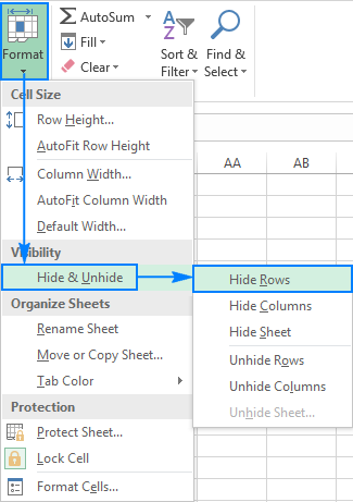
Alternatively, you can go to> Home> Format> Row Height and type 0 in the Row Height box.
In either case, the selected rows are immediately hidden from view.
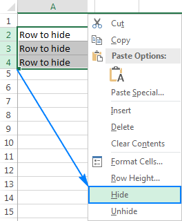
Hide rows using the right-click menu
You can access the Hide command from the right-click menu: right-click on the selected rows and then click Hide.
Excel shortcut to hide rows
If you prefer not to take your hand off the keyboard, you can quickly hide the selected row (s) by pressing this shortcut: Ctrl + 9
How to show hidden rows in Excel
Microsoft Excel has different ways of displaying lines, such as hiding them. Use any of your personal preferences. What makes the difference is the area you choose to instruct Excel to display all hidden rows, special rows, or the first row in a tab.
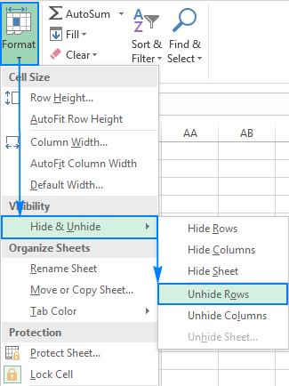
Show hidden rows using ribbon
On the Home tab, in the Cells group, click the Format button, select Hide & Unhide below Visibility, and then click Unhide Rows.
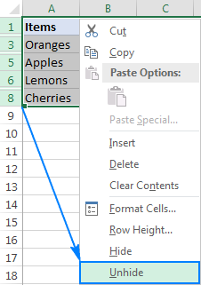
Show hidden rows via right-click menu
You select a group of rows, including the top and bottom rows of the row (s) you want to display, right-click on them, and select Unhide in the list that appears. This method is used to show a hidden line as well as several lines.
For example, to show all the hidden rows between rows 1 and 8, select this group of rows as shown below, right-click and click Unhide:
Shortcut to show hidden rows
Here is the Excel Unhide Rows shortcut: Ctrl + Shift + 9
Pressing this key combination (3 keys simultaneously) shows each row hidden in the selection range.
Show hidden lines by double-clicking
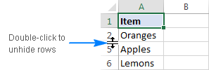
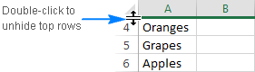
In many cases, the fastest way to display rows in Excel is to double-click on them. The good thing about this method is that you do not need to choose anything. Simply hover your mouse over the hidden row titles and double-click when the mouse pointer turns into a split double arrow.
How to display all lines in Excel
To display all rows on a page, you must select all rows. To do this, you can either:
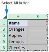
- Click the Select All button (a small triangle in the upper left corner of a tab, at the intersection of row and column titles):
- Press the Select All shortcut key: Ctrl + A
Please note that in Microsoft Excel, this shortcut behaves differently in different situations. If the cursor is empty in a cell, the entire leaf job is selected. But if the cursor is in one of the cells connected to the data, only that group of cells are selected. Press Ctrl + A again to select all cells.
After selecting the entire page, you can display all the rows by doing one of the following:
- Press Ctrl + Shift + 9 (fastest method).
- Select Unhide from the right-click menu (the easiest way to remember nothing).
- On the Home tab, click Format> Unhide Rows.
How to display all lines in Excel
To display all rows and columns, select the entire page as described above, then press Ctrl + Shift + 9 to show hidden rows and Ctrl + Shift + 0 to show hidden columns. Give.
How to display specific rows in Excel
Depending on which rows you want to display, select them as shown below and then apply one of the unhide options discussed above.
To show one or more adjacent rows, select the top row and bottom row (s) you want to display.
To display multiple non-adjacent rows, select all rows between the first and last visible row in the group.
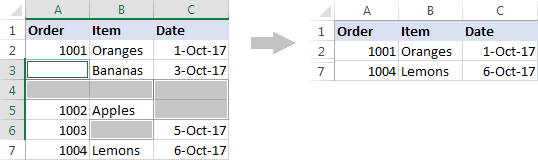
For example, to display rows 3, 7, and 9, select rows 2-10, and then use the ribbon, right-click menu, or keyboard shortcut to display them.
How to display the initial lines
Hiding the first line in Excel is easy, you hide it just like any other line on the page. But when one or more of the above lines are hidden, how can you show them again, given that there is nothing else to choose from?
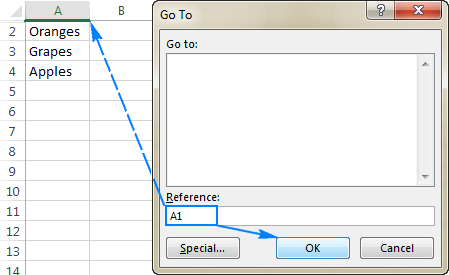
The clue is cell selection A1. All you have to do is type A1 in the Name box and press Enter.
Alternatively, go to Home> Editing, click Find & Select, and then click To Go To. The Go To dialog box appears, type A1 in the Reference box and click OK.
By selecting cell A1, you can display the first hidden row in the usual way, by clicking Format> Unhide Rows on the ribbon, or selecting Unhide from the right-click menu, or pressing the shortcut Ctrl + Shift + 9.
Aside from this common approach, there is another (and faster!) Way to display the first line in Excel. Simply move to the hidden row title and double-click when the mouse cursor turns into a split double arrow:
Tips and tricks to hide and show lines in Excel
As you can see recently, hiding and showing rows in Excel is fast and straightforward. However, in some cases even a simple task can become a challenge. Below are simple solutions to some complex problems.
The Hide rows containing empty cells
Follow these steps to hide rows that contain empty cells:
1. Select the domain containing the empty cells that you want to hide.
2. On the Home tab, in the Editing group, click Find & Select> Go To Special.
3. In the Go To Special dialog box, select the Blanks button and click OK. This selects all empty cells in the range.
4. Press Ctrl + 9 to hide the corresponding rows.
This method works well when you want to hide all rows that have at least one empty cell, as shown in the image below:
If you want to hide empty rows in Excel, ie rows where all cells are empty, use the COUNTBLANK formula.
Hide rows by cell size
Use the Excel Filter feature to hide and display rows based on the number of cells in one or more columns. This feature gives you a handful of predefined filters for text, numbers and dates, as well as the ability to configure a custom filter with the desired criteria.
To display filtered rows, remove the filter from a specific column or all filters on a page.
The Hide unused rows (blank)
If there is a small workspace on the page and a lot of unnecessary empty rows and columns, you can hide unused rows this way:
1. Select the row below the last row with the data (to select the entire row, click on the row tab).
2. Press Ctrl + Shift + Down arrow to expand the selection at the bottom of the tab.
3. Press Ctrl + 9 to hide selected rows.
Hide unused columns in a similar way:
1. Select the empty column after the last column with the data.
2. Press Ctrl + Shift + Right arrow to select other unused columns at the bottom of the tab.
3- To hide the selected columns, press Ctrl + 0. Done!
If you decide to display all cells later, select the full screen, then press Ctrl + Shift + 9 to hold all rows and Ctrl + Shift + 0 to display all columns.
Find all hidden lines on a page
If your worksheet contains hundreds or thousands of lines, it is difficult to identify hidden items. The following trick makes the job easier.
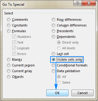
On the Home tab, in the Edit group, select Find & Select> Go To Special. Or press Ctrl + G to open the Go To dialog box, then click Special.
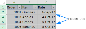
In the Go To Special window, select Visible cells only and click OK.
Select all visible cells and mark the rows adjacent to the hidden rows with a white border:
How to copy visible lines in Excel
Suppose you have hidden several discontinuous lines and now you want to copy the continuous data to another tab or workbook. How can you do this? Select visible lines with the mouse and press Ctrl + C to copy them? But it also copies hidden lines!
To copy visible lines in Excel, you must work differently:
1. Select the visible lines using the mouse.
2. Go to Home> Editing, and select Find & Select> Go To Special.
3. In the Go To Special window, select only the visible cells and click OK. This will select only visible rows.
4. Press Ctrl + C to copy the selected rows.
5. Press Ctrl + V to paste visible rows.
Do not display rows in Excel
If you have trouble displaying rows in your worksheets, it is most likely due to one of the following:
1- The worksheet is protected
Whenever Hide and Unhide features are disabled in Excel, the first thing to check is worksheet protection.
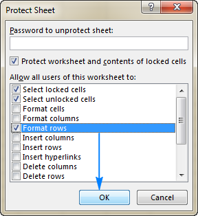
To do this, go to Review> Changes and see if the Unprotect Sheet button is there (this button only appears on protected tabs; in an unprotected worksheet, there is a Protect Sheet button instead). So, if you see the Unprotect Sheet button, click on it.
If you want to keep the user page protected but do not allow the lines to be hidden and visible, click the Protect Sheet button on the Review tab, select Format rows and click OK.
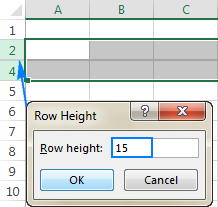
2. The row height is low, but not zero
If the worksheet is not protected, but certain rows still cannot be displayed, check the height of those rows. The point is, if the row height is set slightly, between 0.08 and 1, the row may appear to be hidden, but this is not the case. Such lines cannot be displayed in the usual way. You must change the row height to return them.
To do this, follow these steps:
1. Select a group of lines, including one line above and one line below the problematic line (s).
2. Right-click on them and select Row Height from the menu.
3. Type the desired value in the Row Height box (for example 15) and click OK.
This will make all hidden lines visible again.
If the row height is set to 0.07 or less, such rows usually cannot be displayed without the above manipulations.
3- The problem of not displaying the first line in Excel
If someone has hidden the first row in a tab, you may have trouble returning it because you cannot select the row before it. In this case, select cell A1 as described in the initial rows and then display the row as usual, for example by pressing Ctrl + Shift + 9.
If none of the above works for you, it is possible that the hidden lines are the result of a filter. In this case, clear the filters.
Home > Data Recovery > 2 Methods to Hide or Show Specific Lines in a Line Chart in Your Excel Worksheet
When there are many data series in a worksheet, the corresponding line chart will also be in a mess. In order to make the chart clearer, we have the two methods in this article.
The line chart in Excel can show data and information better. But with many lines in one chart, you will find it hard to check certain lines. In our previous article How to Create a Dynamic Line Chart with Checkboxes in Your Excel Worksheet, we have introduced a method to make the line chart better. And here we have found other two effective methods. Continue reading this article and see how these two methods take effect.
Method 1: Create a Pivot Chart
The pivot chart in Excel is very powerful. You can use it to fulfill many amazing tasks. And here we will show you the steps of using pivot chart to make the line chart better.
- Select the original range in the worksheet.
- And then click the tab “Insert” in the ribbon.
- After that, click the arrow button under the button “PivotTable”.
- In the drop-down menu, only two options are available. Here you need to choose the second option “PivotChart”.

- After that, in the “Create PivotTable with PivotChart” window, set the location that you need to show the chart. Here we will choose a new worksheet.

- When you finish the setting of location, click the button “OK” in the window. Next you will directly come to the new worksheet with the pivot table and the pivot chart.
- In this worksheet, right click in the chart area.
- And then in the new menu, choose the option “Change Chart Type”.

- In the “Change Chart Type” window, you can see that the default chart type is column chart. Here you need to choose the line chart in this window.

- After that, click the button “OK” in the window.
- Now you will also come back to the worksheet. Here you can check the fields in the “Choose fields to add report” area. The field “Date” needs to be always checked. As for other products, you can check them according to your actual need.


Therefore, you can see that using the pivot chart can save you a lot of time and energy. Therefore, the next time you can consider using this method.
Method 2: Use VBA Macros
If you don’t want to create another worksheet or a new pivot table in your worksheet, you can use the VBA macros in the file. Also here you need to combine the VBA macros with the check boxes for the line chart. Before you use the macros, you need first arrange the worksheet.
- In the original worksheet, create the line chart for the data and information.
- And then click the tab “Developer” in the ribbon. If there is no such a tab, you need to add it in the “Excel Options” window.
- Next click the button “Insert” in the toolbar.
- After that, choose the “Check Box” in the drop-down menu.

- And then click in the chart area. Therefore, you have inserted a new check box in the worksheet.
- Next right click the check box.
- In the pop-up menu, change the text into the name of the product “DataNumen Excel Repair”.
- Next adjust the width of the check box so that it can show the whole phrase.

- Repeat the step 2-8 and insert other check boxes for other products. You need to insert the number of check boxes and change their names according to your need.
- Ans then in this step, press the button “Ctrl” on the keyboard and hold it.
- Next use your mouse to select all the check boxes in the chart.
- After that, you can release the button “Ctrl”.
- And then click the tab “Format” in the ribbon.
- After that, click the button “Align” in the toolbar.
- In the drop-down list, choose the options and align those check boxes. Here we will choose “Align Left” and the “Distribute Vertically” in the menu.

- Next, press the “Ctrl” again.
- And then click the line chart. After that, you can also release the button.
- After that, click the button “Group” in the toolbar.
- In the drop-down list, still click “Group”. Therefore, you have grouped those check boxes with the line chart.

- When you finish the setting in the chart, you need to use VBA macros. Here press the button “Alt +F11” on the keyboard to open the Visual Basic window.
- And then insert a new module in the editor.

- In this step, copy the following codes into the new module.


Sub HideShowLine()
  Application.ScreenUpdating = False
  Dim i As Integer
  For i = 1 To 5
    If ActiveSheet.CheckBoxes("Check Box " & i).Value = -4146 Then
      ActiveSheet.ChartObjects("Chart 1").Activate
      ActiveChart.SeriesCollection(i).Format.Line.Visible = msoFalse
    Else
      ActiveSheet.ChartObjects("Chart 1").Activate
      ActiveChart.SeriesCollection(i).Format.Line.Visible = msoTrue
    End If
  Next i
End Sub

Sub AssignMacro()
  Application.ScreenUpdating = False
  Dim i As Integer
  For i = 1 To 5
    ActiveSheet.Shapes.Range(Array("Check Box " & i)).Select
    Selection.OnAction = "HideShowLine"
  Next i
End Sub
There are two macros. The first will hide or show lines according to the condition of the corresponding check boxes. And the second is to assign the first macro to those check boxes. You need to change certain elements in the codes, such as the numbers of the lines, and the name of the chart.
- And then you need to run the second macro. Click in the area of the second macro and press the button “F5” on the keyboard to run it.
Next you can come back to the worksheet. When you check or uncheck the check box, you will see the corresponding lines in the chart.
This method is also very useful. In your actual worksheet, you can also have a try.
A Comparison of the Methods
In this part, we will make a comprehensive comparison of the three methods. And the other method is in the article How to Create a Dynamic Line Chart with Checkboxes in Your Excel Worksheet.
|
Comparison |
Create a Pivot Chart | Use VBA Macros |
Use Check Boxes |
|
Advantages |
This method is very easy to use. And you don’t necessarily need to know the VBA or other functions. | The VBA codes can also be used in other worksheets. You only need to modify certain elements in the codes. | When you don’t know VBA macros and you want to show the result in this ordinary line chart, you can use this method. |
|
Disadvantages |
This method will create the pivot table together with the pivot chart. If you don’t want to create an additional pivot table, you can use other methods. | If you are not familiar with Excel VBA, you will probably meet with problems when changing or running the macros. | This method will actually add a new range in the worksheet. And this will mess up your worksheet. |
All the methods have their advantages and disadvantages. When you need to hide or show lines in a line chart, you can choose one method according to your actual need.
Focus on the Privacy and Security in Excel
In your Excel, not only will there be the data and information that you manually input, but also there will be some private information. This private information is essential. Therefore, you need to pay special attention to your files. Sometimes your files will be damaged by virus or the malicious malware. The result can be very series. Your personal information in the worksheet will be known by someone else. Besides, the data and information will also be damaged. At this moment, you can use a third-party tool to repair Excel xlsx file error. With this tool at hand, you can well protect your important files.
Author Introduction:
Anna Ma is a data recovery expert in DataNumen, Inc., which is the world leader in data recovery technologies, including repair Word docx problem and outlook repair software products. For more information visit www.datanumen.com