
Hide error values and error indicators in cells
Excel for Microsoft 365 Excel 2021 Excel 2019 Excel 2016 Excel 2013 Excel 2010 Excel 2007 More…Less
Let’s say that your spreadsheet formulas have errors that you anticipate and don’t need to correct, but you want to improve the display of your results. There are several ways to hide error values and error indicators in cells.
There are many reasons why formulas can return errors. For example, division by 0 is not allowed, and if you enter the formula =1/0, Excel returns #DIV/0. Error values include #DIV/0!, #N/A, #NAME?, #NULL!, #NUM!, #REF!, and #VALUE!.
Convert an error to zero and use a format to hide the value
You can hide error values by converting them to a number such as 0, and then applying a conditional format that hides the value.
Create an example error
-
Open a blank workbook, or create a new worksheet.
-
Enter 3 in cell B1, enter 0 in cell C1, and in cell A1, enter the formula =B1/C1.
The #DIV/0! error appears in cell A1. -
Select A1, and press F2 to edit the formula.
-
After the equal sign (=), type IFERROR followed by an opening parenthesis.
IFERROR( -
Move the cursor to the end of the formula.
-
Type ,0) – that is, a comma followed by a zero and a closing parenthesis.
The formula =B1/C1 becomes =IFERROR(B1/C1,0). -
Press Enter to complete the formula.
The contents of the cell should now display 0 instead of the #DIV! error.
Apply the conditional format
-
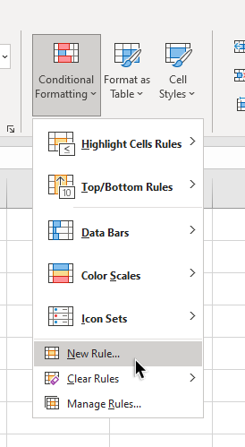
Select the cell that contains the error, and on the Home tab, click Conditional Formatting.
-
Click New Rule.
-
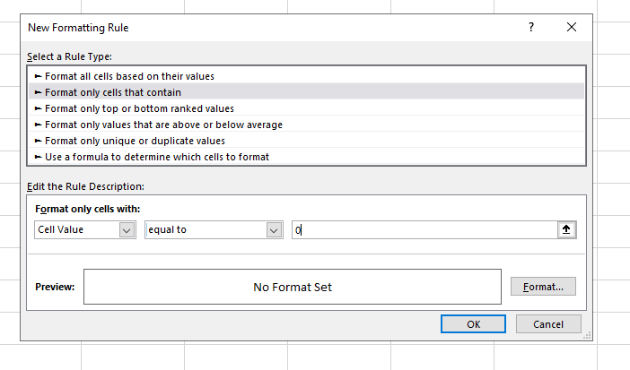
In the New Formatting Rule dialog box, click Format only cells that contain.
-
Under Format only cells with, make sure Cell Value appears in the first list box, equal to appears in the second list box, and then type 0 in the text box to the right.
-
Click the Format button.
-
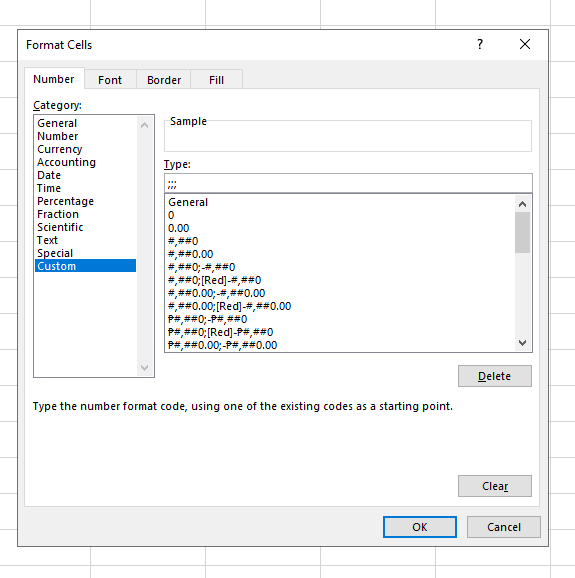
Click the Number tab and then, under Category, click Custom.
-
In the Type box, enter ;;; (three semicolons), and then click OK. Click OK again.
The 0 in the cell disappears. This happens because the ;;; custom format causes any numbers in a cell to not be displayed. However, the actual value (0) remains in the cell.
Use the following procedure to format cells that contain errors so that the text in those cells is displayed in a white font. This makes the error text in these cells virtually invisible.
-
Select the range of cells that contain the error value.
-
On the Home tab, in the Styles group, click the arrow next to Conditional Formatting and then click Manage Rules.
The Conditional Formatting Rules Manager dialog box appears. -
Click New Rule.
The New Formatting Rule dialog box appears. -
Under Select a Rule Type, click Format only cells that contain.
-
Under Edit the Rule Description, in the Format only cells with list, select Errors.
-
Click Format, and then click the Font tab.
-
Click the arrow to open the Color list, and under Theme Colors, select the white color.
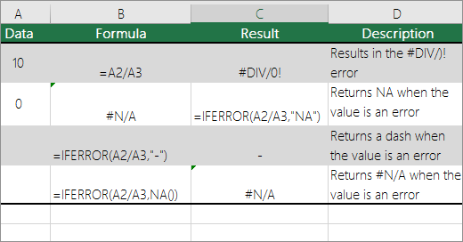
There may be times when you do not want error vales to appear in cells, and would prefer that a text string such as “#N/A,” a dash, or the string “NA” appears instead. To do this, you can use the IFERROR and NA functions, as the following example shows.
Function details
IFERROR Use this function to determine if a cell contains an error or if the results of a formula will return an error.
NA Use this function to return the string #N/A in a cell. The syntax is =NA().
-
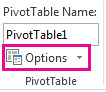
Click the PivotTable report.
The PivotTable Tools appear. -
Excel 2016 and Excel 2013: On the Analyze tab, in the PivotTable group, click the arrow next to Options, and then click Options.
Excel 2010 and Excel 2007: On the Options tab, in the PivotTable group, click the arrow next to Options, and then click Options.
-
Click the Layout & Format tab, and then do one or more of the following:
-
Change error display Select the For error values show check box under Format. In the box, type the value that you want to display instead of errors. To display errors as blank cells, delete any characters in the box.
-
Change empty cell display Select the For empty cells show check box. In the box, type the value that you want to display in empty cells. To display blank cells, delete any characters in the box. To display zeros, clear the check box.
-
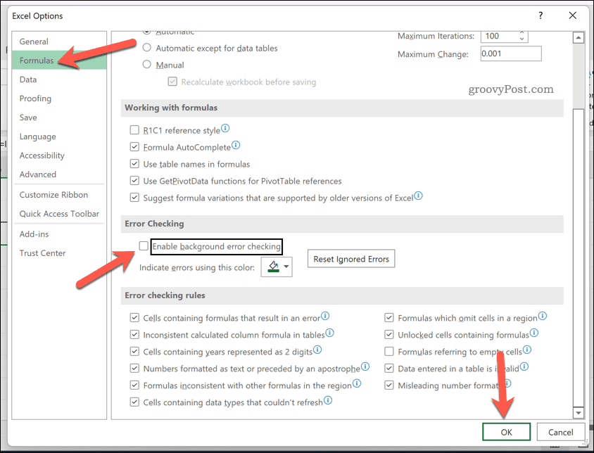
If a cell contains a formula that results in an error, a triangle (an error indicator) appears in the top-left corner of the cell. You can prevent these indicators from being displayed by using the following procedure.

Cell with a formula problem
-
In Excel 2016, Excel 2013, and Excel 2010: Click File > Options >Formulas.
In Excel 2007: Click the Microsoft Office Button
 > Excel Options > Formulas.
 -
Under Error Checking, clear the Enable background error checking check box.
Need more help?
Want more options?
Explore subscription benefits, browse training courses, learn how to secure your device, and more.
Communities help you ask and answer questions, give feedback, and hear from experts with rich knowledge.
At the time of using Excel formulas have you ever encountered error messages like #VALUE! or #DIV/0!? Do you know you can hide errors in Excel worksheet?
Well, the occurrence of such kinds of formula errors is a clear indication that you need to re-check the error source. Whereas in most cases such type of formula error simply shows that the data used by the formulas is not present.
Are you also the one who is looking for some easy tricks to hide error values in Excel? If you don’t know how Excel hide errors then this article is going to be very interesting and informative for you.
Following are some easy tricks to hide errors in Excel.
1# Hide Error Values In A PivotTable Report
2# Hide Error Indicators In Cells
3#Hide Error Values By Turning The Text White
4# Hide Errors With The IFERROR Function
5# Hide All Error Values In Excel With Conditional Formatting
Trick 1# Hide Error Values In A PivotTable Report
- Make a tap over the PivotTable report it will start showing PivotTable Tools.
- Excel 2016/2013: Go to the Analyze tab and then to the PivotTable Now hit the arrow sign present next to the Options, after that choose the Options button.
Excel 2010/2007: From the Options tab>PivotTable group. Hit the arrow sign present next to Options and after that choose the Options.
- Just hit the Layout & Format tab and try any of the following options:
- Change Error Display: From the Format tab choose the “For error values show”. In the appearing box, just assign the value which you want to show in place of errors.
In order to show errors like blank cells, just clear all the characters present in the box.
- Change Empty Cell Display:
From the Format tab choose the “For empty cells show” option. In the appearing box, just assign the value which you want to show in place of errors.
In order to show errors like blank cells, just clear all the characters present in the box. Whereas, to display zeros, just leave the check box empty.
Trick 2# Hide Error Indicators In Cells
If your cell is having a formula which is showing error then you will see a triangle single which is an error indicator. It appears in the cell’s top-left corner and one can easily stop these indicators from appearing by trying the following steps:
- Select the formula cell that is having the problem
- In Excel 2016/ 2013/ 2010: Hit the File> Options >Formulas.
In Excel 2007: Hit the Microsoft Office Button > Excel Options > Formulas.
- In the opened Error Checking dialog box, just clear the check box of Enable background error checking.

Trick 3# Hide Error Values By Turning The Text White
By applying the white color to your text you can easily hide errors in Excel. This will make your text color completely invisible.
- Choose the cells range that has the error value.
- Go to the Home tab and in the Styles group, tap to the arrow sign present next to the Conditional Formatting.

- After that hit the Manage Rules option. This will open the dialog box of Conditional Formatting Rules Manager.
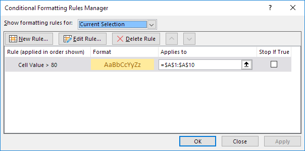
- Tap to the New Rule. After this, you will see a dialog box of New Formatting Rule will get open on your screen.
- From Select a Rule Type section hit the Format only cells that contain.
- Now from the Format only cells with section go to the Edit the Rule Description option and hit the Errors.
- Go to the Format tab, and then make a tap over the Font.
- For opening up, the Color list hit the arrow sign and then from the Theme Colors choose the white color.

Trick 4# Hide Errors With The IFERROR Function
The easiest trick to hide error values in the Excel workbook is by using the IFERROR function. So by making use of the IFERROR function one can very easily replace the error which is appearing with another value or also with the alternative formula.
In the given example, the VLOOKUP function is showing the #N/A error value.
Well, the error has occurred because there is no Office detail assigned for searching. Not only this, it will start causing issues with the total calculation.
The IFERROR function efficiently handles the error value such as, #NAME!, #DIV/0!, #REF! Etc. this needs a value for checking up the error and if the error is encountered what task needs to perform.
In the above-given example, the VLOOKUP function is used for checking up the values, and instead of error “0” will be displayed.
Trick 5# Hide All Error Values In Excel With Conditional Formatting
Excel Conditional Formatting function can also help you in the task of hiding error values. Follow the below-given steps:
1. Choose the data range up to which you are willing to hide the formula errors.
2 Follow this path: Home > Conditional Formatting > New Rule.

3. Now from the opened dialog box of New Formatting Rule you have to select ”Use a formula to determine which cells to format” option which is present within the “Select a Rule Type”.
After that enter the formula: =ISERROR(A1) within the text box of “Format values where this formula is true”. (A1 is 1st cell that is present within the selected range which you can modify as per your need)

4. Hit the Format button this will open the Format Cells dialog box. After that select a white color for cell font from the Font.
Tips: Try to keep the font and background color the same. Suppose you have selected a red color for your background then choose red color also for the font.

5. To close the opened dialog box hit the OK You will see that entire error values will goes hidden at once.


Best Software For Recover Missing Excel Workbook Data
If your Excel workbook data goes corrupted, missing, or deleted then you can make use of the MS Excel Repair Tool. This is the best tool to repair all sorts of issues, corruption, errors in Excel workbooks. This tool allows to easily restore all corrupt Excel file including the charts, worksheet properties cell comments, and other important data.
* Free version of the product only previews recoverable data.
This is a unique tool to repair multiple Excel files at one repair cycle and recovers the entire data in a preferred location. It is easy to use and compatible with both Windows as well as Mac operating systems. This software supports the entire Excel version.
Wrap Up:
Now that you know how to hide error in Excel then do try this in your worksheet.
I Hope this article seems informative to you. But if have any more tricks to share regarding this Excel hide errors techniques then feel free to share it with us on our Facebook and Twitter page.
Good Luck..!


Priyanka is an entrepreneur & content marketing expert. She writes tech blogs and has expertise in MS Office, Excel, and other tech subjects. Her distinctive art of presenting tech information in the easy-to-understand language is very impressive. When not writing, she loves unplanned travels.
Содержание
- Hide error values and error indicators in cells
- Convert an error to zero and use a format to hide the value
- How to correct a #VALUE! error
- Fix the error for a specific function
- Problems with subtraction
- Subtract a cell reference from another
- Or, use SUM with positive and negative numbers
- Subtract a cell reference from another
- Or, use the DATEDIF function
- Problems with spaces and text
- 1. Select referenced cells
- 2. Find and replace
- 3. Replace spaces with nothing
- 4. Replace or Replace all
- 5. Turn on the filter
- 6. Set the filter
- 7. Select any unnamed checkboxes
- 8. Select blank cells, and delete
- 9. Clear the filter
- 10. Result
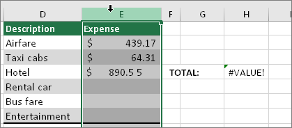
- Example with #VALUE!
- Same example, with ISTEXT
- Other solutions to try
- Select the error
- Click Formulas > Evaluate Formula
- Cell with #VALUE!
- Error hidden by IFERROR
Hide error values and error indicators in cells
Let’s say that your spreadsheet formulas have errors that you anticipate and don’t need to correct, but you want to improve the display of your results. There are several ways to hide error values and error indicators in cells.
There are many reasons why formulas can return errors. For example, division by 0 is not allowed, and if you enter the formula =1/0, Excel returns #DIV/0. Error values include #DIV/0!, #N/A, #NAME?, #NULL!, #NUM!, #REF!, and #VALUE!.
Convert an error to zero and use a format to hide the value
You can hide error values by converting them to a number such as 0, and then applying a conditional format that hides the value.
Create an example error
Open a blank workbook, or create a new worksheet.
Enter 3 in cell B1, enter 0 in cell C1, and in cell A1, enter the formula =B1/C1.
The #DIV/0! error appears in cell A1.
Select A1, and press F2 to edit the formula.
After the equal sign (=), type IFERROR followed by an opening parenthesis.
IFERROR(
Move the cursor to the end of the formula.
Type ,0 ) – that is, a comma followed by a zero and a closing parenthesis.
The formula =B1/C1 becomes =IFERROR(B1/C1 ,0).
Press Enter to complete the formula.
The contents of the cell should now display 0 instead of the #DIV! error.
Apply the conditional format
Select the cell that contains the error, and on the Home tab, click Conditional Formatting.
In the New Formatting Rule dialog box, click Format only cells that contain.
Under Format only cells with, make sure Cell Value appears in the first list box, equal to appears in the second list box, and then type 0 in the text box to the right.
Click the Format button.
Click the Number tab and then, under Category, click Custom.
In the Type box, enter ;;; (three semicolons), and then click OK. Click OK again.
The 0 in the cell disappears. This happens because the ;;; custom format causes any numbers in a cell to not be displayed. However, the actual value (0) remains in the cell.
Use the following procedure to format cells that contain errors so that the text in those cells is displayed in a white font. This makes the error text in these cells virtually invisible.
Select the range of cells that contain the error value.
On the Home tab, in the Styles group, click the arrow next to Conditional Formatting and then click Manage Rules.
The Conditional Formatting Rules Manager dialog box appears.
Click New Rule.
The New Formatting Rule dialog box appears.
Under Select a Rule Type, click Format only cells that contain.
Under Edit the Rule Description, in the Format only cells with list, select Errors.
Click Format, and then click the Font tab.
Click the arrow to open the Color list, and under Theme Colors, select the white color.
There may be times when you do not want error vales to appear in cells, and would prefer that a text string such as “#N/A,” a dash, or the string “NA” appears instead. To do this, you can use the IFERROR and NA functions, as the following example shows.
IFERROR Use this function to determine if a cell contains an error or if the results of a formula will return an error.
NA Use this function to return the string #N/A in a cell. The syntax is = NA().
Click the PivotTable report.
The PivotTable Tools appear.
Excel 2016 and Excel 2013: On the Analyze tab, in the PivotTable group, click the arrow next to Options, and then click Options.
Excel 2010 and Excel 2007: On the Options tab, in the PivotTable group, click the arrow next to Options, and then click Options.
Click the Layout & Format tab, and then do one or more of the following:
Change error display Select the For error values show check box under Format. In the box, type the value that you want to display instead of errors. To display errors as blank cells, delete any characters in the box.
Change empty cell display Select the For empty cells show check box. In the box, type the value that you want to display in empty cells. To display blank cells, delete any characters in the box. To display zeros, clear the check box.
If a cell contains a formula that results in an error, a triangle (an error indicator) appears in the top-left corner of the cell. You can prevent these indicators from being displayed by using the following procedure.
Cell with a formula problem
In Excel 2016, Excel 2013, and Excel 2010: Click File > Options > Formulas.
In Excel 2007: Click the Microsoft Office Button  > Excel Options > Formulas.
Under Error Checking, clear the Enable background error checking check box.
Источник
How to correct a #VALUE! error
#VALUE is Excel’s way of saying, «There’s something wrong with the way your formula is typed. Or, there’s something wrong with the cells you are referencing.» The error is very general, and it can be hard to find the exact cause of it. The information on this page shows common problems and solutions for the error. You may need to try one or more of the solutions to fix your particular error.

Fix the error for a specific function
Don’t see your function in this list? Try the other solutions listed below.
Problems with subtraction
If you’re new to Excel, you might be typing a formula for subtraction incorrectly. Here are two ways to do it:
Subtract a cell reference from another
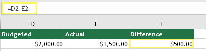
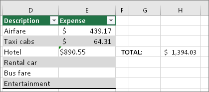
Type two values in two separate cells. In a third cell, subtract one cell reference from the other. In this example, cell D2 has the budgeted amount, and cell E2 has the actual amount. F2 has the formula =D2-E2.
Or, use SUM with positive and negative numbers
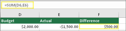
Type a positive value in one cell, and a negative value in another. In a third cell, use the SUM function to add the two cells together. In this example, cell D6 has the budgeted amount, and cell E6 has the actual amount as a negative number. F6 has the formula =SUM(D6,E6).
If you’re using Windows, you might get the #VALUE! error when doing even the most basic subtraction formula. The following might solve your problem:
First do a quick test. In a new workbook, type a 2 in cell A1. Type a 4 in cell B1. Then in C1 type this formula =B1-A1. If you get the #VALUE! error, go to the next step. If you don’t get the error, try other solutions on this page.
In Windows, open your Region control panel.
Windows 10: Click Start, type Region, and then click the Region control panel.
Windows 8: At the Start screen, type Region, click Settings, and then click Region.
Windows 7: Click Start and then type Region, and then click Region and language.
On the Formats tab, click Additional settings.
Look for the List separator. If the List separator is set to the minus sign, change it to something else. For example, a comma is a common list separator. The semicolon is also common. However, another list separator might be more appropriate for your particular region.
Open your workbook. If a cell contains a #VALUE! error, double-click to edit it.
If there are commas where there should be minus signs for subtraction, change them to minus signs.
Repeat this process for other cells that have the error.
Subtract a cell reference from another
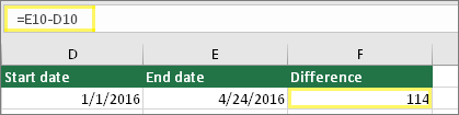
Type two dates in two separate cells. In a third cell, subtract one cell reference from the other. In this example, cell D10 has the start date, and cell E10 has the End date. F10 has the formula =E10-D10.
Or, use the DATEDIF function
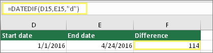
Type two dates in two separate cells. In a third cell, use the DATEDIF function to find the difference in dates. For more information on the DATEDIF function, see Calculate the difference between two dates.
Make your date column wider. If your date is aligned to the right, then it’s a date. But if it’s aligned to the left, this means the date isn’t really a date. It’s text. And Excel won’t recognize text as a date. Here are some solutions that can help this problem.
Check for leading spaces
Double-click a date that is being used in a subtraction formula.
Put your cursor at the beginning and see if you can select one or more spaces. Here’s what a selected space looks like at the beginning of a cell: 
If your cell has this problem, proceed to the next step. If you don’t see one or more spaces, go to the next section on checking your computer’s date settings.
Select the column that contains the date by clicking its column header.
Click Data > Text to Columns.
Click Next twice.
On Step 3 of 3 of the wizard, under Column data format, click Date.
Choose a date format, and then click Finish.
Repeat this process for other columns to ensure they don’t contain leading spaces before dates.
Check your computer’s date settings
Excel uses your computer’s date system. If a cell’s date isn’t entered using the same date system, then Excel won’t recognize it as a true date.
For example, let’s say that your computer displays dates as mm/dd/yyyy. If you typed a date like that in a cell, Excel would recognize it as a date and you’d be able to use it in a subtraction formula. However, if you typed a date like dd/mm/yy, then Excel wouldn’t recognize that as a date. Instead, it would treat it as text.
There are two solutions to this problem: You could change the date system that your computer uses to match the date system you want to type in Excel. Or, in Excel you could create a new column and use the DATE function to create a true date based on the date stored as text. Here’s how to do that assuming your computers date system is mm/dd/yyy and your text date is 31/12/2017 in cell A1:
Create a formula like this: =DATE(RIGHT(A1,4),MID(A1,4,2),LEFT(A1,2))
The result would be 12/31/2017.
If you want the format to appear like dd/mm/yy, press CTRL+1 (or  + 1 on the Mac).
Choose a different locale that uses the dd/mm/yy format, for example, English (United Kingdom). When you’re done applying the format, the result would be 31/12/2017 and it would be a true date, not a text date.
Note: The formula above is written with the DATE, RIGHT, MID, and LEFT functions. Please notice that it is written with an assumption that the text date has two characters for days, two characters for months, and four characters for year. You may need to customize the formula to suit your date.
Problems with spaces and text
Often #VALUE! occurs because your formula refers to other cells that contain spaces, or even trickier: hidden spaces. These spaces can make a cell look blank, when in fact they are not blank.
1. Select referenced cells
Find cells that your formula is referencing and select them. In many cases removing spaces for an entire column is a good practice because you can replace more than one space at a time. In this example, clicking the E selects the entire column.
2. Find and replace
On the Home tab, click Find & Select > Replace.
3. Replace spaces with nothing
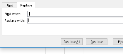
In the Find what box, type a single space. Then, in the Replace with box, delete anything that might be there.
4. Replace or Replace all
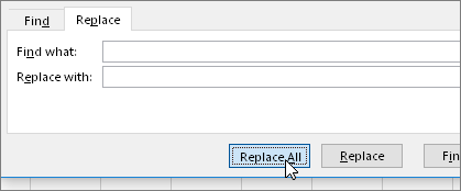
If you are confident that all spaces in the column should be removed, click Replace All. If you’d like to step through and replace spaces with nothing on an individual basis, you can click Find next first, and then click Replace when you are confident the space isn’t needed. When you’re done, the #VALUE! error may be resolved. If not, go to the next step.
5. Turn on the filter
Sometimes there are hidden characters other than spaces that can make a cell appear blank, when it’s not really blank. Single apostrophes within a cell can do this. To get rid of these characters in a column, turn on the filter by going to Home > Sort & Filter > Filter.
6. Set the filter

Click the filter arrow  , and then deselect Select all. Then, select the Blanks checkbox.
7. Select any unnamed checkboxes
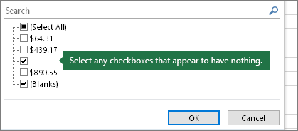
Select any check boxes that don’t have anything next to them, like this one.
8. Select blank cells, and delete

When Excel brings back the blank cells, select them. Then press the Delete key. This will clear any hidden characters in the cells.
9. Clear the filter
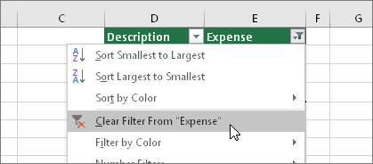
Click the filter arrow , and then click Clear filter from. so that all cells are visible.
10. Result
If spaces were the culprit of your #VALUE! error then hopefully your error has been replaced by the formula result, as shown here in our example. If not, repeat this process for other cells that your formula refers to. Or, try other solutions on this page.
Note: In this example, notice that cell E4 has a green triangle and the number is aligned to the left. This means the number is stored as text. This may cause more problems later. If you see this problem, we recommend converting numbers stored as text to numbers.
Text or special characters within a cell can cause the #VALUE! error. But sometimes it’s hard to see which cells have these problems. Solution: Use the ISTEXT function to inspect cells. Please note that ISTEXT doesn’t resolve the error, it simply finds cells that might be causing the error.
Example with #VALUE!
Here’s an example of a formula that has a #VALUE! error. This is likely due to cell E2. There is a special character that appears as a small box after «00.» Or as the next picture shows, you could use the ISTEXT function in a separate column to check for text.
Same example, with ISTEXT
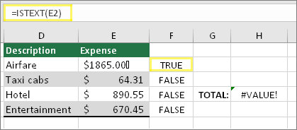
Here the ISTEXT function was added in column F. All cells are fine except the one with the value of TRUE. This means cell E2 has text. To resolve this, you could delete the cell’s contents and retype the value of 1865.00. Or you could also use the CLEAN function to clean out characters, or use the REPLACE function to replace special characters with other values.
After using CLEAN or REPLACE, you’ll want to copy the result, and use Home > Paste > Paste Special > Values. You might also have to convert numbers stored as text to numbers.
Formulas with math operations like + and * may not be able to calculate cells that contain text or spaces. In this case, try using a function instead. Functions will often ignore text values and calculate everything as numbers, eliminating the #VALUE! error. For example, instead of =A2+B2+C2, type =SUM(A2:C2). Or, instead of =A2*B2, type =PRODUCT(A2,B2).
Other solutions to try
Select the error

First select the cell with the #VALUE! error.
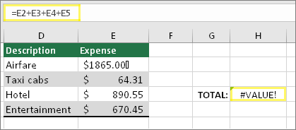
Click Formulas > Evaluate Formula
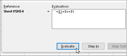
Click Formulas > Evaluate Formula > Evaluate. Excel will step through the parts of the formula individually. In this case the formula =E2+E3+E4+E5 breaks because of a hidden space in cell E2. You can’t see the space by looking at cell E2. However, you can see it here. It shows as » «.
Sometimes you just want to replace the #VALUE! error with something else like your own text, a zero or a blank cell. In this case you can add the IFERROR function to your formula. IFERROR will check to see if there’s an error, and if so, replace it with another value of your choice. If there isn’t an error, your original formula will be calculated. IFERROR will only work in Excel 2007 and later. For earlier versions you can use IF(ISERROR()).
Warning: IFERROR will hide all errors, not just the #VALUE! error. Hiding errors isn’t recommended because an error is often a sign that something needs to be fixed, not hidden. We don’t recommend using this function unless you are absolutely certain your formula works the way that you want.
Cell with #VALUE!
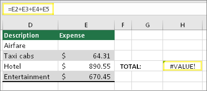
Here’s an example of a formula that has a #VALUE! error due to a hidden space in cell E2.
Error hidden by IFERROR
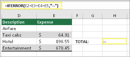
And here’s the same formula with IFERROR added to the formula. You can read the formula as: «Calculate the formula, but if there’s any kind of error, replace it with two dashes.» Note that you could also use «» to display nothing instead of two dashes. Or you could substitute your own text, such as: «Total Error».
Unfortunately, you can see that IFERROR doesn’t actually resolve the error, it simply hides it. So be certain that hiding the error is better than fixing it.
Your data connection may have become unavailable at some point. To fix this, restore the data connection, or consider importing the data if possible. If you don’t have access to the connection, ask the creator of the workbook to make a new file for you. The new file ideally would only have values, and no connections. They can do this by copying all the cells, and pasting only as values. To paste as only values, they can click Home > Paste > Paste Special > Values. This eliminates all formulas and connections, and therefore would also remove any #VALUE! errors.
If you’re not sure what to do at this point, you can search for similar questions in the Excel Community Forum, or post one of your own.
Источник
While working with formulas in spreadsheets, we might get error values. These error values are often shown in the cells as error indicators. Sometimes, they are helpful in resolving errors but other times when errors need not be corrected, these error values just make the spreadsheet look cluttered. In such a situation, it is better to hide these error indicators to not only make the spreadsheet look clean but also to prevent these errors from stopping other formulas to work correctly. Let us discuss the different ways in which we can do that but first let us look at the problem statement with an example.
Hiding Error Values and Indicators in MS Excel
Open a new excel sheet and follow the steps given below.
Step 1: Go to the Math and Trig section on the formulas tab and click on the quotient option from the drop-down menu. You must see a pop-up like this:

Select the Quotient formula
Step 2: In this pop-up, enter 4 in the numerator and 0 in the denominator.

Enter values in the pop-up
Step 3: Click ok. You will get an error like this:

The div error
You can see how this error is indicated with an exclamatory mark since division by 0 is not defined. Some other error values can be #NAME?, #NULL!, and #REF!, etc.
Before we discuss the various ways in which we can hide these error values, let us first see how to deal with error indicators.
Change the Excel settings to Hide Error Indicators
As you can see in the above example, whenever a cell contains an error, a triangle appears in the top-left corner. This is nothing but an error indicator. Follow the steps given below to hide these error indicators:
Step 1: Go to file tab and select options.

Step 1
Step 2: A dialog box will appear. In this box, go to the formulas section and deselect the enable background checking box under the error checking section.

Step 2
Step 3: Click ok.
This was to hide the error indicators, now onto error values.
Use the IFERROR function to Convert the Error to Zero
Let us first enter =DIV(6/3) in the cell A1 of an excel spreadsheet.

Create an error
Then, click on enter and you will see an error like this:

#NAME error
To hide this error, follow the steps given below:
Step 1: Select cell A1 and click the F2 button. This is let you edit the formula.
Step 2: Now, to this formula, add the following function along with a 0 at the end as shown below.

IFERROR function
Step 3: Once you click enter, you will see a 0 in place of the #NAME? error.
If you wish, you can hide this 0 as well by using conditional formatting.
Hide the Zero with the help of the Conditional Format
Follow the below steps in continuation to hide the 0 present in cell A1.
Step 1: Select cell A1 and click on the conditional formatting option present under the home tab.

Conditional formatting option on the home tab
Step 2: From the list, select the New Rule option. You will see a dialog box like this:

New Rule Dialog box
Step 3: Inside this dialog box, select Format only cells that contain option from the rule type, and under the edit rule description section, the first cell should contain Cell value, the second cell should contain equal to and enter 0 in the last cell.

New Formatting rule
Step 4: Click the format button. You will see a dialog box with the name Format Cells appears. In this dialog box, click on the number tab, and select custom from the category section. Also, under the type section, enter three semicolons like this ;;; as shown below:

Format Cells
Step 5: Now, click ok. Click ok again. You can see that the 0 in cell A1 disappears after this.
We can also use the conditional formatting option to turn the text white so that the erroneous text is not visible.
Use Conditional format to turn text white and hide error values
To turn the text white using a conditional format, follow the below steps:
Note that we are using the same =DIV(6/3) error as above to explain this example.
Step 1: Select the cell or the range of cells containing error and click on the conditional formatting option present under the home tab.

Conditional formatting
Step 2: From the list, select the New Rule option. You will see a dialog box like this:
New formatting rule
Step 3: Inside this dialog box, select Format only cells that contain option from the rule type, and in the edit rule description section, select errors from the first dropdown.

New formatting rule
Step 4: Click on format. A new dialog box will appear. Go to the font section in this dialog box.

Font
Step 5: On the font tab, choose a white color from the color drop-down.

Color drop down
Step 6: Click ok. Click ok again.
Replace the Error with NA or a dash
We can use the IFERROR and NA functions to replace an error with the string NA, #N/A, or a dash(-).
The IFERROR function
The IFERROR function of excel is used to check if there is an error in a cell or a formula. If the error is found, the IFERROR function returns the value you specify. Otherwise, it simply returns the result of the formula.
Syntax
IFERROR(formula, replacement_value)
The function takes two arguments.
1. formula – It is the formula that has to be evaluated for errors.
2. replacement_value – It is the value that is returned when the formula evaluates to an error. The error can be #N/A, #REF!, #NULL!, #NAME?, #DIV/0! and #VALUE!.
Use the IFERROR function to replace the error with a dash or the string NA
Let us try this out on the first example error that we saw above.
Step 1: Double-click in cell A1 to edit the formula. Edit the formula as follows:

Edit the formula
Step 2: Press enter. You will see that the error is replaced by the string NA.

NA appears
If you want to display a dash instead of the string NA, then change the formula as follows:
=IFERROR(QUOTIENT(4,0), “-“)
The NA functions
This function simply returns #N/A. This is an error value that means ‘no value is available’. This helps in marking empty cells.
Syntax
NA()
This function has no arguments.
Use the NA function along with the IFERROR function to replace the error with #N/A
Just like we replaced an error value with a string or dash with the help of the IFERROR function, we can replace it with the value #N/A with the help of these two formulae:
=IFERROR(QUOTIENT(4,0), NA())
This is done below:
Step 1: Double-click in the cell A1 to edit the formula. Edit the formula as follows:

The formula
Step 2: Press Enter, and then you get the result.

The result
We can use the IFERROR function and conditional formatting to hide all error values in a Microsoft Excel spreadsheet.
This technique will be useful for cleaning up a table that may be prone to errors.
Common Excel errors include the #DIV/0, #REF, and #VALUE errors. While these error outputs are incredibly useful for finding bugs in your spreadsheet, they may be distracting. This is especially the case with spreadsheets where errors are expected, such as a table with missing values.
For example, let’s say we have a table where a column is the quotient of two other values. If the divisor is zero, then our column will return a #DIV/0 error. While dividing by zero is considered an error in mathematics, a blank cell may be easier to read for users.
With this situation in mind, is it possible to hide error values from your worksheet?
Excel’s IFERROR function can help catch these errors when they happen. IFERROR works by allowing the user to specify a custom result to return when a formula generates an error.
If no error occurs, then the formula returns the standard result. We can combine the IFERROR function with conditional formatting to return a blank cell without changing the actual value returned.
For example, we can have IFERROR return a 0 when it encounters an error. Afterward, we can create a custom rule that simply returns a blank cell when IFERROR returns 0.
Now that we know when to use the IFERROR function, let’s see how the formula works on an actual spreadsheet.
A Real Example of Hiding All Error Values in Excel
Let’s take a look at a real example of the IFERROR function being used in an Excel spreadsheet.
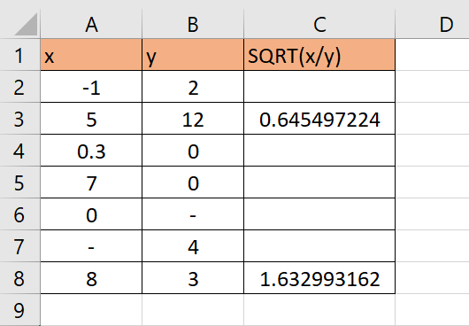
The spreadsheet below has multiple error values, including #NUM!, #REF!, and #VALUE. We can use conditional formatting and Excel functions to make the spreadsheet much less cluttered and easier to read.
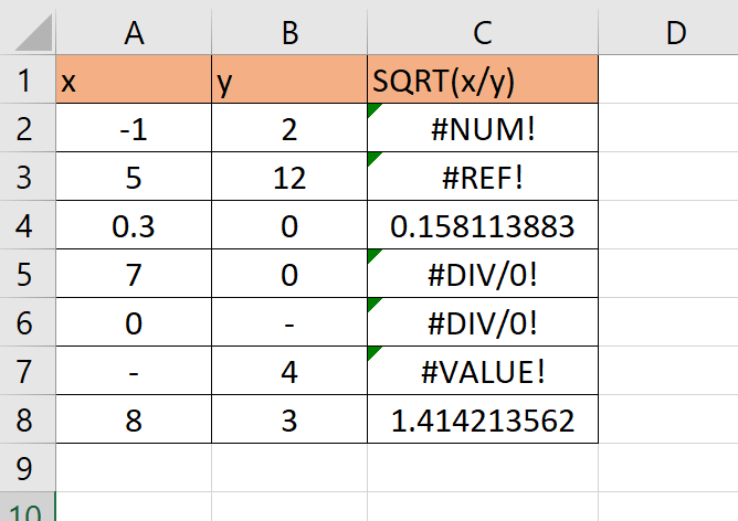
After using a custom conditional formatting rule, our table should now show a blank cell if the formula returns an error.
You can make your own copy of the spreadsheet above using the link attached below.
If you want to try out this technique yourself in Excel, read the next section for a step-by-step guide on hiding error values.
This section will guide you through each step needed to hide all error values in your Excel spreadsheet. You’ll learn how to wrap any equation with an IFERROR function to catch any potential errors. Afterward, we’ll explain how we can use conditional formatting to display blank cells.
Follow these steps to understand how to hide error values in Excel:
- First, we’ll need to select the cell that may output an error. In this example, cell C2 can return an error for any number of reasons.
For example, trying to get the square root of a negative number will result in a #NUM! error. If we divide by zero, we’ll end up with a #DIV/0! error.

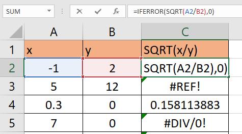
- Next, we’ll have to wrap our main formula with an
IFERRORfunction. In the example below, we’ve placed our main functionSQRT(A2/B2)into ourIFERRORfunction as the first argument. Our second argument will be the digit 0. This means that our formula will return 0 if the first argument causes an error.

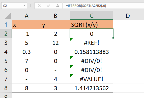
- Hit the Enter key to evaluate the function.

- We can then drag down our formula to fill the rest of our column with cells that use
IFERROR.

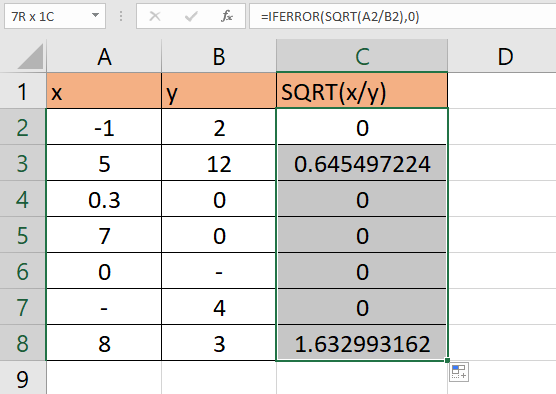
- Next, select the range where you want to add conditional formatting rules. In this example, we’ve selected the cell range C2:C8.

- Look for the Conditional Formatting icon in the Home tab. Click on the New Rule… option found in the dropdown menu.

- Select the ‘Format only cells that contain’ option as the Rule Type. For the rule description, we’d like to only format cells with a value equal to 0. Click on the Format… button to define the format used for our rule.

- In the Format Cells dialog, navigate to the Number tab. Select Custom as the category.
In the Type box, type ‘;;;’ then click on OK. The three semicolons indicate a format that hides cell values.

- The final table should now hide all error values because of our custom conditional formatting rule.


Frequently Asked Questions (FAQ)
- Can I use the IFERROR function to return my own default value?
Yes. You can use IFERROR to return text values such as “NA”, “N/A”, “None”, or even a simple ‘-’ hyphen. You can even use an alternate formula in case the first argument returns an error.
That’s all you need to remember to start using the IFERROR function and conditional formatting together in Excel. This step-by-step guide shows how you can hide error output in your sheets easily.
The IFERROR function is another useful function in Excel that you can use to improve the overall look of your spreadsheet. With so many other Excel functions available, you can surely find one that works for you.
Are you interested in learning more about what Excel can do?
Make sure to subscribe to our newsletter to be the first to know about the latest guides and tutorials from us.

Get emails from us about Excel.
Our goal this year is to create lots of rich, bite-sized tutorials for Excel users like you. If you liked this one, you’d love what we are working on! Readers receive ✨ early access ✨ to new content.

Hi! I’m a Software Developer with a passion for data analytics. Google Sheets has helped me empower my teams to make data-driven decisions. There’s always something new to learn, so let’s explore how you can make life so much easier with spreadsheets!

An error in Excel is a sign that a calculation or formula has failed to provide a result. You can hide Excel errors in a few different ways. Here’s how.
The perfect Microsoft Excel spreadsheet doesn’t contain errors—or does it?
Excel will throw out an error message when it can’t complete a calculation. There are a number of reasons why, but it’ll be up to you to figure it out and solve it. Not every error can be solved, however.
If you don’t want to fix the problem, or you simply can’t, you can decide to ignore the Excel errors instead. You might decide to do this if the error doesn’t change the results you’re seeing, but you don’t want to see the message.
If you’re unsure how to ignore all errors in Microsoft Excel, follow the steps below.
How to Hide Error Indicators in Excel
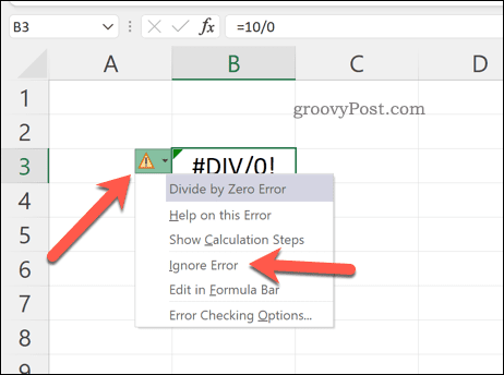
Used a formula incorrectly? Rather than return an incorrect result, Excel will throw up an error message. For example, you might see a #DIV/0 error message if you try to divide a value by zero. You may also see other on-screen error indicators, such as warning icons next to the cell containing the error.
You can’t hide the error message without altering the formula or function you’re using but you can hide the error indicator. This will make it less obvious that the spreadsheet data is incorrect.
To quickly hide error indicators in Excel:
- Open your Excel spreadsheet.
- Select the cell (or cells) containing the error messages.
- Click the warning icon that appears next to the cells when selected.
- From the drop-down, select Ignore Error.

The warning icon will disappear, ensuring the error appears more discreetly in your spreadsheet. If you want to hide the error itself, you’ll need to follow the steps below.
How to Use IFERROR in Excel to Hide Errors
The best way to stop error messages from appearing in Excel is to use the IFERROR function. IFERROR uses IF logic to check a formula before returning a result.
For example, if a cell returns an error, return a value. If it doesn’t return an error, return the correct result. You can use IFERROR to hide error messages and make your Excel spreadsheet error-free (visually, at least).
The structure for an IFERROR formula is =IFERROR(value,value_if_error). You’ll need to replace value with a nested function or calculation that may contain an error. Replace value_if_error with the message or value that Excel should return instead of an error message.
If you’d rather see no error message appearing, use an empty text string (eg. “”) instead.
To use IFERROR in Excel:
- Open your Excel spreadsheet.
- Select an empty cell.
- In the formula bar, type your IFERROR formula (eg. =IFERROR(10/0,””)
- Press Enter to view the result.


IFERROR is a simple but powerful tool for hiding Excel errors. You can nest multiple functions within it, but to test it out, make sure the function you’re using is designed to return an error. If the error doesn’t appear, you’ll know it works.
How to Disable Error Reporting in Excel
If you want to disable error reporting in Excel completely, you can. This ensures that your spreadsheet remains free of errors, but you don’t need to use workarounds like IFERROR to do it.
You might decide to do this to prepare a spreadsheet for printing (even if there are errors). As your data might become incomplete or incorrect with error reporting disabled in Excel, we wouldn’t recommend disabling it for production use.
To disable error reporting in Excel:
- Open your Excel document.
- On the ribbon, press File.

- In File, press Options (or More > Options).

- In Excel Options, press Formulas.
- Uncheck the Enable background error checking checkbox.
- Press OK to save.


Resolving Issues in Microsoft Excel
If you’ve followed the steps above, you should be able to ignore all errors in an Excel spreadsheet. While it isn’t always possible to fix a problem in Excel, you don’t need to see it. IFERROR works well, but if you want a quick fix, you can always disable error reporting entirely.
Excel is a powerful tool, but only if it’s working properly. You may need to troubleshoot further if Excel keeps crashing, but an update or restart will usually fix it.
If you have a Microsoft 365 subscription, you can also try repairing your Office installation. If the file’s at fault, try repairing your document files instead.
![]()

Содержание
- Н / Д появляется в электронной таблице Excel
- Скрытие значений ошибок
- Пример
- Метод 1. Использование форматирования для скрытия ошибки
- Использование функции ЕСЛИОШИБКА
- Использование функции = ЕСЛИОШИБКА
- Использование условного форматирования
- Метод 2 — превратить текст в белый цвет
Я бывший учитель математики, которому часто давали любую работу, требующую использования Excel. Таким образом, я научился многим трюкам.
Н / Д появляется в электронной таблице Excel
Скрытие значений ошибок
Иногда при использовании Microsoft Excel вы обнаруживаете, что в одной из ваших ячеек появилось значение ошибки. Это может быть связано с тем, что вы используете формулу, которая пыталась разделить на 0 (в этом случае появится # DIV / 0), или, возможно, ваша формула связана с функцией ВПР, которая не может найти совпадение для ваших данных (в котором case # N / A появится). Это всего лишь два из нескольких кодов ошибок, которые могут появиться в Excel.
Но зачем их скрывать? Почему бы просто не удалить формулу? Что ж, особенно в случае ошибки # N / A, вы, возможно, настроили свою электронную таблицу с формулами, готовыми для данных, которые вы будете вводить в будущем. В этом случае вам нужны готовые формулы, но если на всем листе написано # N / A, это может выглядеть неаккуратно и непрофессионально. В этой статье я приведу несколько различных способов решения этой проблемы.

Пример
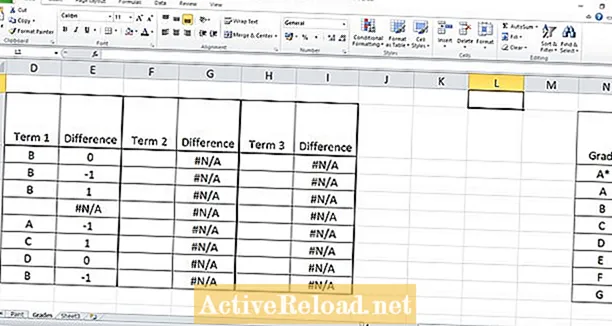
Взгляните на таблицу, которую я установил на картинке выше. В таблице показаны восемь школьников и их целевые оценки на конец года (розовый столбец). В столбце «Семестр 1» показаны их фактические оценки за этот семестр. Следующий столбец заполняется формулой, включающей функцию ВПР.
Я использовал функцию ВПР и таблицу справа, чтобы преобразовать буквенные оценки учащихся в числа, чтобы затем я мог отображать разницу между их целевыми и фактическими оценками в столбце под названием «Разница».
Это сработало для большинства учащихся первого семестра. Мы можем быстро увидеть разницу между их целевыми и фактическими оценками, а также определить, кому нужна помощь, кто выше целевого и т. Д.
К сожалению, Джон Сёртиз отсутствовал, когда класс проводил тест в конце семестра, поэтому у него нет фактической оценки за семестр 1. Затем в столбце «Разница» было возвращено # N / A, поскольку формула ВПР не может найти ничего для соответствовать. Термины 2 и 3 столбца одинаковы для всех.
Это выглядит беспорядочно, и я хочу скрыть все сообщения об ошибках, не удаляя формулу из всех этих ячеек.
Давайте посмотрим, как это сделать.
Метод 1. Использование форматирования для скрытия ошибки
Используя функцию ЕСЛИОШИБКА, вы можете преобразовать любые ошибки в числа, а затем использовать условное форматирование, чтобы скрыть их.
Использование функции ЕСЛИОШИБКА

Использование функции = ЕСЛИОШИБКА
Функция = ЕСЛИОШИБКА работает, возвращая элемент по вашему выбору, если ваша формула возвращает ошибку.
В моем примере на картинке выше я ввел следующую формулу:
= ЕСЛИОШИБКА (ВПР ($ C6; $ N $ 2: $ O $ 10,2; ЛОЖЬ) -ВПР (D6; $ N $ 2: $ O $ 10,2; ЛОЖЬ); 100)
У меня та же формула ВПР, что и раньше, заключенная в скобки функции = ЕСЛИОШИБКА:
= ЕСЛИОШИБКА (моя формула,
Затем следует запятая и 100. Я выбрал 100, чтобы Excel возвращал в случае появления ошибки. Я мог бы выбрать что угодно и поставить его после запятой, но вы сразу поймете, почему я выбрал номер.
Окончательная формула выглядит так:
= ЕСЛИОШИБКА (моя формула, 100).
Excel теперь вернет ответ на мою формулу, если она работает, или 100, если она не работает.
Чтобы завершить исправление, нам теперь нужно добавить некоторое форматирование, чтобы любые 100 были скрыты.

Использование условного форматирования
1. Выделите все свои ячейки и нажмите «Условное форматирование», затем «Новое правило».
2. Выберите «Форматировать только ячейки, которые содержат», затем убедитесь, что в раскрывающемся списке под ним указано «равно», и введите рядом с ним «100». (Это указывает Excel форматировать любое поле, содержащее 100).

3. Щелкните «Формат», а затем вкладку «Число». В меню категории нажмите «Пользовательский» и введите «;;;» в поле типа. Это говорит Excel взять любое поле, содержащее 100, и оставить его пустым.
4. Щелкните «ОК». Все ячейки # Н / Д теперь должны быть пустыми, но продолжат работать в обычном режиме, как только вы введете данные, позволяющие формуле иметь ответ.

Метод 2 — превратить текст в белый цвет
Этот метод немного менее удовлетворителен, но намного быстрее и проще. Значок # N / A по-прежнему будет отображаться, но, поскольку текст будет белым, вы не сможете его увидеть.
1. На главной вкладке выберите «Условное форматирование», а затем нажмите «Новое правило», как мы это делали в способе 1.
2. Выберите «Форматировать только содержащиеся ячейки», а затем выберите «Ошибки» в раскрывающемся списке.

3. Щелкните «Форматировать» и перейдите на вкладку «Шрифт». В раскрывающемся цветном меню измените его на «белый» (или в зависимости от цвета фона вашей ячейки), а затем нажмите «ОК».
Ваши сообщения об ошибках исчезнут.
Эта статья точна и правдива, насколько известно автору. Контент предназначен только для информационных или развлекательных целей и не заменяет личного или профессионального совета по деловым, финансовым, юридическим или техническим вопросам.

Your Excel formulas can occasionally produce errors that don’t need fixing. However, these errors can look untidy and, more importantly, stop other formulas or Excel features from working correctly. Fortunately, there are ways to hide these error values.
Hide Errors with the IFERROR Function
The easiest way to hide error values on your spreadsheet is with the IFERROR function. Using the IFERROR function, you can replace the error that’s shown with another value, or even an alternative formula.
In this example, a VLOOKUP function has returned the #N/A error value.

This error is due to there not being an office to look for. A logical reason, but this error is causing problems with the total calculation.
The IFERROR function can handle any error value including #REF!, #VALUE!, #DIV/0!, and more. It requires the value to check for an error and what action to perform instead of the error if found.
In this example, the VLOOKUP function is the value to check and “0” is displayed instead of the error.
Using “0” instead of the error value ensures the other calculations and potentially other features, such as charts, all work correctly.
Background Error Checking
If Excel suspects an error in your formula, a small green triangle appears in the top-left corner of the cell.
Note that this indicator does not mean that there is definitely an error, but that Excel is querying the formula you’re using.
Excel automatically performs a variety of checks in the background. If your formula fails one of these checks, the green indicator appears.
When you click on the cell, an icon appears warning you of the potential error in your formula.
Click the icon to see different options for handling the supposed error.
In this example, the indicator has appeared because the formula has omitted adjacent cells. The list provides options to include the omitted cells, ignore the error, find more information, and also change the error check options.
To remove the indicator, you need to either fix the error by clicking “Update Formula to Include Cells” or ignore it if the formula is correct.
Turn Off the Excel Error Checking
If you do not want Excel to warn you of these potential errors, you can turn them off.
Click File > Options. Next, select the “Formulas” category. Uncheck the “Enable Background Error Checking” box to disable all background error checking.
Alternatively, you can disable specific error checks from the “Error Checking Rules” section at the bottom of the window.
By default, all of the error checks are enabled except “Formulas Referring to Empty Cells.”
More information about each rule can be accessed by positioning the mouse over the information icon.
Check and uncheck the boxes to specify which rules you would like Excel to use with the background error checking.
When formula errors do not need fixing, their error values should be hidden or replaced with a more useful value.
Excel also performs background error checking and queries mistakes it thinks you’ve made with your formulas. This is useful but specific or all error checking rules can be disabled if they interfere too much.
READ NEXT
- › How to Find Circular References in Microsoft Excel
- › How to Count Cells in Microsoft Excel
- › How to Hide Errors in Google Sheets
- › How to Find a Value’s Position With MATCH in Microsoft Excel
- › The Basics of Structuring Formulas in Microsoft Excel
- › How to Use the IS Functions in Microsoft Excel
- › How to Fix Common Formula Errors in Microsoft Excel
- › HoloLens Now Has Windows 11 and Incredible 3D Ink Features