Hide all rows vba excel - Word и Excel - помощь в работе с программами

When working with Excel, you may find yourself in situations where you may need to hide or unhide certain rows or columns using VBA.

Consider, for example, the following situations (mentioned by Excel guru John Walkenbach in the Excel 2016 Bible) where knowing how to quickly and easily hide rows or columns with a macro can help you:

You’ve been working on a particular Excel workbook. However, before you send it by email to its final users, you want to hide certain information.
You want to print an Excel worksheet. However, you don’t want the print-out to include certain details or calculations.

Knowing how to do the opposite (unhide rows or columns using VBA) can also prove helpful in certain circumstances. A typical case where knowing how to unhide rows or columns with VBA can save you time is explained by Excel MVP Mike Alexander in Excel Macros for Dummies:

When you’re auditing a spreadsheet that you did not create, you often want to ensure that you’re getting a full view of the spreadsheet’s contents. To do so, all columns and rows must not be hidden.

Regardless of whether you want to hide or unhide cells or columns, I’m here to help you. In this tutorial, I provide an easy-to-follow introduction to the topic of using Excel VBA to hide or unhide rows or columns.

Further to the above, I provide 16 ready-to-use macro examples that you can use right now to hide or unhide rows and columns.

This Excel VBA Hide or Unhide Columns and Rows Tutorial is accompanied by an Excel workbook containing the data and macros I use in the examples below. You can get immediate free access to this example workbook by subscribing to the Power Spreadsheets Newsletter.

The following table of contents lists the main sections of this blog post:

Excel VBA Constructs To Hide Rows Or Columns
- Hide Or Unhide With The Range.Hidden Property
- Specify Row Or Column To Hide Or Unhide Using VBA
Excel VBA Code Examples To Hide Columns
- VBA Code Example #1: Hide A Column
- VBA Code Example #2: Hide Several Contiguous Columns
- VBA Code Example #3: Hide Several Non-Contiguous Columns
Excel VBA Code Examples To Hide Rows
- VBA Code Example #4: Hide A Row
- VBA Code Example #5: Hide Several Contiguous Rows
- VBA Code Example #6: Hide Several Non-Contiguous Rows
Excel VBA Code Examples To Unhide Columns
- VBA Code Example #7: Unhide A Column
- VBA Code Example #8: Unhide Several Contiguous Columns
- VBA Code Example #9: Unhide Several Non-Contiguous Columns
- VBA Code Examples #10 And #11: Unhide All Columns In A Worksheet
Excel VBA Code Examples To Unhide Rows
- VBA Code Example #12: Unhide A Row
- VBA Code Example #13: Unhide Several Contiguous Rows
- VBA Code Example #14: Unhide Several Non-Contiguous Rows
- VBA Code Examples #15 And #16: Unhide All Columns In A Worksheet
Conclusion
Books Referenced In This Excel VBA Tutorial

Let’s start by taking a look at the…

Excel VBA Constructs To Hide Rows Or Columns

If your purpose if to hide or unhide rows or columns using Excel VBA, you’ll need to know how to specify the following 2 aspects using Visual Basic for Applications:

The cell range you want to hide or unhide.
When you specify this range, you’re answering the question: Which are the rows or columns that Excel VBA should work with?
Whether you want to (i) hide or (ii) unhide the range you specify in #1 above.
The question you’re answering in this case is: Should Excel VBA hide or unhide the specified cells?

The following sections introduce some VBA constructs that you can use for purposes of specifying the 2 items above. More precisely:

In the first part, I explain what VBA property you can use for purposes of specifying whether Excel VBA should (i) hide or (ii) unhide the cells its manipulating.
In the second part, I introduce some VBA constructs you that you may find helpful for purposes of specifying the rows or columns you want to work with.
For further information about the Range object, and how to create appropriate references, please refer to this thorough tutorial on the topic.

Hide Or Unhide With The Range.Hidden Property

In order to hide or unhide rows or columns, you generally use the Hidden property of the Range object.

The following are the main characteristics of the Range.Hidden property:

It indicates whether the relevant row(s) or column(s) are hidden.
It’s a read/write property. Therefore, you can both (i) fetch or (ii) modify its current setting.

The syntax of Range.Hidden is as follows:

expression.Hidden

“expression” represents a Range object. Therefore, throughout the rest of this VBA tutorial, I use the following simplified syntax:

Range.Hidden

The Range object you specify when working with the Hidden property is important because of the following:

If you’re modifying the property setting, this is the Range that you want to hide or unhide.
If you’re reading the property, this is the Range whose property setting you want to know.

When you specify the cell range you want to hide or unhide, specify the whole row or column. I explain how you can easily do this below.

How To Hide Rows Or Columns With The Range.Hidden Property

If you want to hide rows or columns, set the Hidden property to True.

The basic structure of the basic statement that you must use for these purposes is as follows:

Range.Hidden = True

How To Unhide Rows Or Columns With The Range.Hidden Property

If your objective is to unhide rows or columns, set the Range.Hidden property to False.

In this case, the basic structure of the relevant VBA statement is as follows:

Range.Hidden = False

Specify Row Or Column To Hide Or Unhide Using VBA

In order to be able to hide or unhide rows or columns, you need to have a good knowledge of how to specify which rows or columns Excel should hide or unhide.

In the following sections, I introduce several VBA properties that you can use for these purposes. These properties are commonly used for purposes of creating macros that hide or unhide rows or columns. Therefore, you’ll likely find them useful in many situations.

The following are the properties I explain below:

Worksheet.Range.
Worksheet.Cells.
Worksheet.Columns.
Worksheet.Rows.
Range.EntireRow.
Range.EntireColumn.

The last 2 properties (Range.EntireRow and Range.EntireColumn) are particularly important. As I mention above, when you hide a row or a column using the Range.Hidden property, you usually refer to the whole row or column. Range.EntireRow and Range.EntireColumn allow you to create such a reference. Therefore, you’ll be using these 2 properties often when creating macros that hide or unhide rows and columns.

The following descriptions are a relatively basic introduction to the topic of column and cell references in VBA.

Worksheet.Range Property

The main purpose of the Worksheet.Range property is to return a Range object representing either:

A single cell; or
A cell range.

The Worksheet.Range property has the following 2 syntax versions:

expression.Range(Cell)

expression.Range(Cell1, Cell2)

Which of the above versions you use depends on the characteristics of the Range object you want Visual Basic for Applications to return. Let’s take a closer look at them to understand how you can choose which one to use:

Syntax #1: expression.Range(Cell)

The first syntax version of Worksheet.Range is as follows:

expression.Range(Cell)

Within this statement, the relevant definitions are as follows:

expression: A Worksheet object.
Cell: A required parameter. It represents the range you want to work with.

In order to simplify the statement, I replace “expression” with “Worksheet” as follows:

Worksheet.Range(Cell)

The Cell parameter has the following main characteristics:

As a general rule, Cell is a string specifying a cell range address or a named cell range. In this case, you generally specify Cell using A1-style references.
You can use any of the following operators:
Colon (:): The range operator. You can use colon (:) to refer to (i) entire rows, (ii) entire columns, (iii) ranges of contiguous cells, or (iv) ranges of non-contiguous cells.

Space ( ): The intersection operator. You usually use space ( ) to refer to cells that are common to 2 separate ranges (their intersection).

Comma (,): The union operator. You can use comma (,) to combine several ranges. You may find this particularly useful when working with ranges of non-contiguous rows or columns.

Syntax #2: expression.Range(Cell1, Cell2)

The second syntax version of the Worksheet.Range property is as follows:

expression.Range(Cell1, Cell2)

Some of the comments I make above regarding the first syntax version (expression.Range(Cell)) continue to apply. The following are the relevant items within this statement:

expression: A Worksheet object.
Cell1: The cell in the upper-left corner of the range you want to work with.
Cell2: The cell in the lower-right corner of the range.

Just as in the case of syntax #1 above, I simplify the statement as follows:

Worksheet.Range(Cell1, Cell2)

If you’re working with this version of the Range property, you can specify the parameters (Cell1 and Cell2) in the following ways:

As Range objects. These objects can include, for example, (i) a single cell, (ii) an entire column, or (iii) an entire row.
An address string.
A range name.

How To Refer To An Entire Row Or Column With the Worksheet.Range Property

You can easily create a reference to an entire row or column using the following items:

The first syntax of the Worksheet.Range property (Worksheet.Range(Cell)).
The range operator (:).
The relevant (i) row number(s), or (ii) column letter(s).

More precisely, you can refer to entire rows using a statement of the following form:

Worksheet.Range(“RowNumber1:RowNumber2”)

“RowNumber1” and “RowNumber2” are the number of the row(s) you’re referring to. If you’re referring to a single row, “RowNumber1” and “RowNumber2” are the same.

Similarly, you can create a reference to entire columns by using the following syntax:

Worksheet.Range(“ColumnLetter1:ColumnLetter2”)

“ColumnLetter1” and “ColumnLetter2” are the letters of the column you want to refer to. When you want to refer to a single column, “ColumnLetter1” and “ColumnLetter2” are the same.

Worksheet.Cells Property

The basic purpose of the Worksheet.Cells property is to return a Range object representing all the cells within a worksheet.

The basic syntax of Worksheet.Cells is as follows:

expression.Cells

“expression” represents a Worksheet object. Therefore, I simplify the syntax as follows:

Worksheet.Cells

In this blog post, I show how you can use the Cells property to return absolutely all of the cells within the relevant Excel worksheet. The basic structure of the statements you can use for these purposes is as follows:

Worksheet.Cells

This statement simply follows the basic syntax of the Worksheet.Cells property I introduce above.

Worksheet.Columns Property

The main purpose of the Worksheet.Columns property is to return a Range object representing all columns in a worksheet (the Columns collection).

The following is the basic syntax of Worksheet.Columns:

expression.Columns

“expression” represents a Worksheet object. Therefore, I simplify as follows:

Worksheet.Columns

Worksheet.Rows Property

The Worksheet.Rows property is materially similar to the Worksheet.Columns property I explain above. The main difference between Worksheet.Rows and Worksheet.Columns is as follows:

Worksheet.Columns works with columns
Worksheet.Rows works with rows.

Therefore, Worksheet.Rows returns a Range object representing all rows in a worksheet (the Rows collection).

The syntax of the Rows property is as follows:

expression.Rows

“expression” represents a Worksheet object. Considering this, I simplify the syntax as follows:

Worksheet.Rows

Range.EntireRow Property

The following are the main characteristics of the Range.EntireRow property:

Is a read-only property. Therefore, you can use it to get its current setting.
It returns a Range object.
The Range object it returns represents the entire row(s) that contain the range you specify.

Let’s take a look at the syntax of Range.EntireRow to understand this better:

expression.EntireRow

“expression” represents a Range object. Therefore, I simplify the syntax as follows:

Range.EntireRow

As I explain in #3 above, the EntireRow property returns a Range object representing the entire row(s) containing the range you specify in the first item (Range) of this statement.

Range.EntireColumn Property

The Range.EntireColumn property is substantially similar to the Range.EntireRow property I explain above. The main difference is between EntireRow and EntireColumn is as follows:

EntireRow works with rows.
EntireColumn works with columns.

Therefore, the main characteristics of Range.EntireColumn are as follows:

Is read-only.
It returns a Range object.
The returned Range object represents the entire column(s) containing the range you specify.

The syntax of Range.EntireColumn is substantially the same as that of Range.EntireRow:

expression.EntireColumn

Since “expression” represents a Range object, I can simplify this as follows:

Range.EntireColumn

Such a statement returns a Range object that represents the entire column(s) containing the range you specify in the first item (Range) of the statement.

Now, let’s take a look at some practical examples of VBA code that you can use to hide or unhide rows and columns. We start with…

All of the macro examples below work with a worksheet called “Sheet1” within the active workbook. The reference to this worksheet is built by using the Workbook.Worksheets property (Worksheets(“Sheet1”)).

In most situations, you’ll be working with a different worksheet or several worksheets. For these purposes, you can replace “Worksheets(“Sheet1″)” with the appropriate object reference.

VBA Code Example #1: Hide A Column

You can use a statement of the following form to hide one column:

Worksheets(“Sheet1”).Range(“ColumnLetter:ColumnLetter”).EntireColumn.Hidden = True

The statement proceeds roughly as follows:

Worksheets(“Sheet1”).Range(“ColumnLetter:ColumnLetter”).EntireColumn: Returns the entire column whose letter you specify.
Hidden = True: Sets the Hidden property to True.

This statement is composed of the following items:

Worksheets(“Sheet1”): The Workbook.Worksheets property returns Sheet1 in the active workbook.
Range(“ColumnLetter:ColumnLetter”): The Worksheet.Range property returns a range of cells composed of the column identified with ColumnLetter.
EntireColumn: The Range.EntireColumn property returns the entire column you specify with ColumnLetter.
Hidden = True: The Range.Hidden property is set to True.
This property setting applies to the column returned by items #1 to #3 above. It results in Excel hiding that column.

The following statement is a practical example of how to hide a column. It hides column A (Range(“A:A”)).

Worksheets(“Sheet1”).Range(“A:A”).EntireColumn.Hidden = True

The following sample macro (Example_1_Hide_Column) uses the statement above:

VBA Code Example #2: Hide Several Contiguous Columns

You can use the basic syntax that I introduce in the previous example #1 in order to hide several contiguous columns:

Worksheets(“Sheet1”).Range(“ColumnLetter1:ColumnLetter2”).EntireColumn.Hidden = True

For these purposes, you only need to make 1 change:

Instead of using a single column letter (ColumnLetter) as in the case above (column “A”), specify the following:

ColumnLetter1: Letter of the first column you want to hide.
ColumnLetter2: Letter corresponding to the last column you want to hide.

The following sample statement hides columns A to E (Range(“A:E”)):

Worksheets(“Sheet1”).Range(“A:E”).EntireColumn.Hidden = True

The following macro example (Example_2_Hide_Contiguous_Columns) uses the sample statement above:

VBA Code Example #3: Hide Several Non-Contiguous Columns

The previous 2 examples rely on the range operator (:) when using the Worksheet.Range property.

You can further extend these examples by using the union operator (,). More precisely, the union operator allows you to easily hide several non-contiguous columns.

The basic structure of the statement you can use for these purposes is as follows:

Worksheets(“Sheet1”).Range(“ColumnLetter1:ColumnLetter2,ColumnLetter3:ColumnLetter4,…,ColumnLetter#:ColumnLetter##”).EntireColumn.Hidden = True

Let’s take a closer look at the item that changes vs. the previous examples (Range(“ColumnLetter1:ColumnLetter2,ColumnLetter3:ColumnLetter4,…,ColumnLetter#:ColumnLetter##”)). For these purposes, the column letters you specify have the following meaning:

ColumnLetter1: Letter of first column of first contiguous column range you want to hide.
ColumnLetter2: Letter of last column of first contiguous range to hide.
ColumnLetter3: Letter of first column of second column range you’re hiding.
ColumnLetter4: Letter of last column of second contiguous range you want to hide.
…
ColumnLetter#: Letter of first column of last contiguous column range Excel should hide.
ColumnLetter##: Letter of last column within last column range VBA hides.

In other words, you specify the columns to hide in the following steps:

Group all the columns you want to hide in groups of columns that are contiguous to each other.
For example, if you want to hide columns A, B, C, D, E, G, H, I, L, M, N and O, group them as follows: (i) A to E, (ii) G to I, and (iii) L to O.
Specify the first and last column of each of these groups of contiguous columns using the range operator (:). This is pretty much the same you do in the previous examples #1 and #2.
In the example above, the 3 groups of contiguous columns become “A:E”, “G:I” and “L:O”.
Separate each of these groups from the others by using the union operator (,).
Continuing with the example above, the whole item becomes “A:E,G:I,L:O”.

The following sample VBA statement hides columns (i) A to E, (ii) G to I, and (iii) L to O:

Worksheets(“Sheet1”).Range(“A:E,G:I,L:O”).EntireColumn.Hidden = True

The following Sub procedure example (Example_3_Hide_NonContiguous_Columns) uses the statement above:

Excel VBA Code Examples To Hide Rows

The following 3 examples are substantially similar to those in the previous section (which hide columns). The main difference is that the following macros work with rows.

VBA Code Example #4: Hide A Row

A statement of the following form allows you to hide a single row:

Worksheets(“Sheet1”).Range(“RowNumber:RowNumber”).EntireRow.Hidden = True

The process followed by this statement is as follows:

Worksheets(“Sheet1”).Range(“RowNumber:RowNumber”).EntireRow: Returns the entire row whose number you specify.
Hidden = True: Sets the Range.Hidden property to True.

The statement is composed by the following items:

Worksheets(“Sheet1”): The Workbook.Worksheets property returns Sheet1 of the active workbook.
Range(“RowNumber:RowNumber”): The Worksheet.Range property returns a range of cells. This range is composed of the row identified with RowNumber.
EntireRow: The Range.EntireRow property returns the entire row specified by RowNumber.
Hidden = True: Sets the Hidden property to True.
The property setting is applied to the row returned by items #1 to #3 above. The result is that Excel hides that particular row.

The following sample statement uses the syntax I describe above to hide row 1:

Worksheets(“Sheet1”).Range(“1:1”).EntireRow.Hidden = True

The following macro example (Example_4_Hide_Row) uses this statement:

VBA Code Example #5: Hide Several Contiguous Rows

You can easily extend the basic syntax that I introduce in the previous example #4 for purposes of hiding several contiguous rows:

Worksheets(“Sheet1”).Range(“RowNumber1:RowNumber2”).EntireRow.Hidden = True

The only difference between this statement and the one in example #4 above is the way in which you specify the row numbers (RowNumber1 and RowNumber2). More precisely:

In the previous example, you specify a single row number (RowNumber). This results in Excel hiding a single row.
In this case, you specify 2 row numbers (RowNumber1 and RowNumber2). Excel hides all the rows from (and including) RowNumber1 to (and including) RowNumber2.

Therefore, if you use the statement above, the relevant definitions are as follows:

RowNumber1: Number of first row you hide.
RowNumber2: Number of last row you hide.

The following example VBA statement hides rows 1 through 5 (Range(“1:5”)):

Worksheets(“Sheet1”).Range(“1:5”).EntireRow.Hidden = True

The sample macro below (Example_5_Hide_Contiguous_Rows) uses the sample statement above:

VBA Code Example #6: Hide Several Non-Contiguous Rows

If you take the statements I provide in examples #4 and #5 above one step further by using the union operator (,), you can easily hide several non-contiguous rows.

In this case, the basic structure of the statement you can use is as follows:

Worksheets(“Sheet1”).Range(“RowNumber1:RowNumber2,RowNumber3:RowNumber4,…,RowNumber#:RowNumber##”).EntireRow.Hidden = True

The whole statement is pretty much the same as in the previous example. The items that change are the RowNumbers. When using this syntax, their meaning is as follows:

RowNumber1: Number of first row of first contiguous row range you’re hiding.
RowNumber2: Number of last row within first contiguous row range to hide.
RowNumber3: Number of first row within second contiguous row range you want to hide.
RowNumber4: Number of last row of second contiguous row range Excel hides.
…
RowNumber#: Number of first row of last contiguous row range to hide.
RowNumber##: Number of last row within last contiguous row range to be hidden with VBA.

The following example of VBA code hides rows (i) 1 to 5, (ii) 7 to 10, and (iii) 12 to 15:

Worksheets(“Sheet1”).Range(“1:5,7:10,12:15”).EntireRow.Hidden = True

The following sample Sub procedure (Example_6_Hide_NonContiguous_Rows) uses the statement above:

Excel VBA Code Examples To Unhide Columns

The basic structure of the statements you use to hide or unhide a cell range is virtually the same. More precisely:

If you want to hide a cell range, the basic structure of the statement you use is as follows:

Range.Hidden = True
If you want to unhide a cell range, the basic statement structure is as follows:

Range.Hidden = False

The only thing that changes between these 2 statements is the setting of the Range.Hidden property. In order to hide the cell range, you set it to True. To unhide the cell range, you set it to False.

As a consequence of the above, several of the following statements to unhide columns are virtually the same as those I explain above to hide them.

Below, I show how you can unhide all columns in a worksheet. I don’t explain the structure of these macro examples above.

VBA Code Example #7: Unhide A Column

A statement of the following form allows you to unhide one column:

Worksheets(“Sheet1”).Range(“ColumnLetter:ColumnLetter”).EntireColumn.Hidden = False

This statement structure is virtually the same as that you can use to hide a column. The only difference is that, to unhide the column, you set the Range.Hidden property to False (Hidden = False).

When using this statement structure, “ColumnLetter” is the letter of the column you want to unhide.

The following sample VBA statement unhides column A (Range(“A:A”)):

Worksheets(“Sheet1”).Range(“A:A”).EntireColumn.Hidden = False

The following example macro (Example_7_Unhide_Column) contains the statement above:

VBA Code Example #8: Unhide Several Contiguous Columns

You can use the following statement form to unhide several contiguous columns:

Worksheets(“Sheet1”).Range(“ColumnLetter1:ColumnLetter2”).EntireColumn.Hidden = True

This statement is substantially the same as the one you use to hide several contiguous columns. In order to unhide the columns (vs. hiding them), you set the Hidden property to False (Hidden = False).

When unhiding several contiguous columns, ColumnLetter1 and ColumnLetter2 represent the following:

ColumnLetter1: Letter of the first column to unhide.
ColumnLetter2: Letter of the last column you want to unhide.

The following practical example of a VBA statement unhides columns A to E (Range(“A:E”)):

Worksheets(“Sheet1”).Range(“A:E”).EntireColumn.Hidden = True

This statement appears in the sample macro below (Example_8_Unhide_Contiguous_Columns):

VBA Code Example #9: Unhide Several Non-Contiguous Columns

A statement with the following structure allows you to unhide several non-contiguous columns:

Worksheets(“Sheet1”).Range(“ColumnLetter1:ColumnLetter2,ColumnLetter3:ColumnLetter4,…,ColumnLetter#:ColumnLetter##”).EntireColumn.Hidden = False

The statement is virtually the same to the one that you can use to hide several non-contiguous columns. To unhide the columns, this statement sets the Range.Hidden property to False (Hidden = False).

When specifying the letters of the columns to be unhidden, consider the following definitions:

ColumnLetter1: First column of first group of contiguous columns to unhide.
ColumnLetter2: Last column of first group of columns to unhide.
ColumnLetter3: First column of second group of contiguous columns that Excel unhides.
ColumnLetter4: Last column within second group of contiguous columns you want to unhide.
…
ColumnLetter#: First column within last group of contiguous columns that VBA unhides.
ColumnLetter##: Last column of last group of contiguous columns to unhide.

The following statement example unhides columns (i) A to E, (ii) G to I, and (iii) L to O:

Worksheets(“Sheet1”).Range(“A:E,G:I,L:O”).EntireColumn.Hidden = False

The following sample macro (Example_9_Unhide_NonContiguous_Columns) contains the statement above:

VBA Code Examples #10 And #11: Unhide All Columns In A Worksheet

In some situations, you may want to ensure that all the columns in a worksheet are unhidden. The following VBA code examples help you do this:

VBA Code Example #10: Unhide All Columns In A Worksheet Using The Worksheet.Cells Property

The following statement works with the Worksheet.Cells property on the process of unhiding all the columns in a worksheet:

Worksheets(“Sheet1”).Cells.EntireColumn.Hidden = False

This VBA statement proceeds as follows:

Worksheets(“Sheet1”).Cells.EntireColumn: Returns all columns within Sheet1 of the active workbook.
Hidden = False: Sets the Hidden property to False.

The statement is composed of the following items:

Worksheets(“Sheet1”): The Workbook.Worksheets property returns Sheet1 from the active workbook.
Cells: The Worksheet.Cells property returns all the cells within the applicable worksheet.
EntireColumn: The Range.EntireColumn property returns the entire column for all the columns in the worksheet.
Hidden = False: The Range.Hidden property is set to False.
This setting of the Hidden property applies to the columns returned by items #1 to #3 above. The final result is Excel unhiding all the columns in the worksheet.

The following macro example (Example_10_Unhide_All_Columns) unhides all columns in Sheet1 of the active workbook:

VBA Code Example #11: Unhide All Columns In A Worksheet Using The Worksheet.Columns Property

As an alternative to the previous code example #10, the following statement relies on the Worksheet.Columns property during the process of unhiding all the columns of the worksheet:

Worksheets(“Sheet1”).Columns.EntireColumn.Hidden = False

This statement proceeds in roughly the same way as that in the previous example:

Worksheets(“Sheet1”).Columns.EntireColumn: Returns all the columns of Sheet1 of the active workbook.
Hidden = False: Sets Range.Hidden to False.

The following are the main items within this statements:

Worksheets(“Sheet1”): The Workbook.Worksheets property returns Sheet1 of the active workbook.
Columns: The Worksheet.Columns property returns all the columns within the applicable worksheet.
EntireColumn: The Range.EntireColumn property returns all entire columns within the worksheet.
Hidden = False: The Hidden property is set to False.
Since the Range.Hidden property applies to the columns returned by items #1 to #3 above, Excel unhides all the columns in the worksheet.

The following sample Sub procedure (Example_11_Unhide_All_Columns) unhides all the columns in Sheet1 of the active workbook:

Excel VBA Code Examples To Unhide Rows

As I explain above, the basic structure of the statements you use to hide or unhide a range of rows is virtually the same.

At a basic level, you only change the setting of the Range.Hidden property as follows:

To hide rows, you set Hidden to True (Range.Hidden = True).
To unhide rows, you set Hidden to False (Range.Hidden = False).

Therefore, several of the following sample VBA statements to unhide rows follow the same basic structure and logic as the ones above (which hide rows).

Below, I provide some (new) VBA code examples to unhide all rows in a worksheet.

VBA Code Example #12: Unhide A Row

The following statement structure allows you to unhide a row:

Worksheets(“Sheet1”).Range(“RowNumber:RowNumber”).EntireRow.Hidden = False

This structure follows the form and process I describe above for purposes of hiding a row. However, in this particular case, you set the Range.Hidden property to False (Hidden = False). This results in Excel unhiding the relevant row.

When you use this statement structure, “RowNumber” is the number of the row you want to unhide.

The following example of a VBA statement unhides row 1:

Worksheets(“Sheet1”).Range(“1:1”).EntireRow.Hidden = False

Check out the following sample macro (Example_12_Unhide_Row), which contains this statement:

VBA Code Example #13: Unhide Several Contiguous Rows

If you use the following statement structure, you can easily hide several contiguous rows:

Worksheets(“Sheet1”).Range(“RowNumber1:RowNumber2”).EntireRow.Hidden = False

This statement structure and logic is substantially the same as that I explain above for hiding contiguous rows. The only difference is the setting of the Range.Hidden property. In order to unhide the rows, you set it to False in the statement above (Hidden = False).

When you’re using the structure above, bear in mind the following definitions:

RowNumber1: Number of the first row you want to hide.
RowNumber2: Number of the last row Excel hides.

The following sample statement unhides rows 1 to 5 (Range(“1:5”)):

Worksheets(“Sheet1”).Range(“1:5”).EntireRow.Hidden = False

The macro example below (Example_13_Unhide_Contiguous_Rows) uses this statement:

VBA Code Example #14: Unhide Several Non-Contiguous Rows

You can use the following statement structure for purposes of unhiding several non-contiguous rows:

Worksheets(“Sheet1”).Range(“RowNumber1:RowNumber2,RowNumber3:RowNumber4,…,RowNumber#:RowNumber##”).EntireRow.Hidden = False

The statement structure is substantially the same as that you can use to hide several non-contiguous rows. For purposes of unhiding the rows, set the Hidden property to False (Hidden = False).

Further to the above, remember the following definitions:

RowNumber1: Number of first row of first row range to unhide.
RowNumber2: Number of last row of first row range you want to unhide.
RowNumber3: Number of first row within second range that Excel unhides.
RowNumber4: Number of last row of second contiguous row range you’re unhiding.
…
RowNumber#: Number of first row in last contiguous row range to unhide with VBA.
RowNumber##: Number of last row within last row range you want to unhide.

The following statement sample unhides rows (i) 1 to 5, (ii) 7 to 10, and (iii) 12 to 15:

Worksheets(“Sheet1”).Range(“1:5,7:10,12:15”).EntireRow.Hidden = False

You can check out the following macro example (Example_14_Unhide_Non_Contiguous_Rows), which uses this statement:

VBA Code Examples #15 And #16: Unhide All Columns In A Worksheet

If you want to unhide all the rows within a worksheet, you can use the following sample macros:

VBA Code Example #15: Unhide All Rows In A Worksheet Using The Worksheet.Cells Property

The following statement relies on the Worksheet.Cells property for purposes of unhiding all the rows in a worksheet:

Worksheets(“Sheet1”).Cells.EntireRow.Hidden = False

This VBA statement proceeds as follows:

Worksheets(“Sheet1”).Cells.EntireRow: Returns the all rows within Sheet1 in the active workbook.
Hidden = False: Sets the Hidden property to False.

The statement is composed of the following items:

Worksheets(“Sheet1”): The Workbook.Worksheets property returns Sheet1 from within the active workbook.
Cells: The Worksheet.Cells property returns all the cells within the relevant worksheet.
EntireRow: The Range.EntireRow property returns the entire row for all the rows in the worksheet.
Hidden = False: The Hidden property is set to False.
This setting of the Range.Hidden property applies to the rows returned by items #1 to #3 above. The final result is Excel unhiding all the rows in the worksheet.

The following macro example (Example_15_Unhide_All_Rows) unhides all rows in Sheet1:

VBA Code Example #16: Unhide All Rows In A Worksheet Using The Worksheet.Rows Property

The following VBA statement uses the Worksheet.Rows property when unhiding all the rows in a worksheet. You can use this as an alternative to the previous example #15:

Worksheets(“Sheet1”).Rows.EntireRow.Hidden = False

This statement proceeds in roughly the same way as that in the previous example:

Worksheets(“Sheet1”).Rows.EntireRow: Returns all the rows in Sheet1 of the active workbook.
Hidden = False: Sets the Hidden property to False.

The following are the main items within this statements:

Worksheets(“Sheet1”): The Workbook.Worksheets property returns Sheet1 in the active workbook.
Rows: The Worksheet.Rows property returns all the rows within the worksheet you’re working with.
EntireRow: The Range.EntireRow property returns the entire row for all rows within the worksheet.
Hidden = False: The Range.Hidden property is set to False.
The Hidden property applies to the rows returned by items #1 to #3 above. Therefore, the statement results in Excel unhiding all the rows in the worksheet.

The sample macro that appears below (Example_16_Unhide_All_Rows) unhides all rows within Sheet1 by using the statement I explain above:

Conclusion

After reading this Excel VBA tutorial you have enough knowledge to start creating macros that hide or unhide rows or columns.

More precisely, you’ve read about the following topics:

The Range.Hidden property, which you can use to indicate whether a row or column is hidden or unhidden.
How to use the following VBA properties for purposes of specifying the row(s) or column(s) you want to hide or unhide:
- Worksheet.Range.
- Worksheet.Cells.
- Worksheet.Columns.
- Worksheet.Rows.
- Range.EntireRow.
- Range.EntireColumn.

You also saw 16 macro examples to hide or unhide rows or columns that you can easily adjust and start using right now. The examples of VBA code I provide above can help you do any of the following:

Hide any of the following:
- A column.
- Several contiguous columns.
- Several non-contiguous columns.
- A row.
- Several contiguous rows.
- Several non-contiguous rows.
Unhide any of the following:
- A column.
- Several contiguous columns.
- Several non-contiguous columns.
- All the columns in a worksheet.
- A row.
- Several contiguous rows.
- Several non-contiguous rows.
- All the rows in a worksheet.

This Excel VBA Hide or Unhide Columns and Rows Tutorial is accompanied by an Excel workbook containing the data and macros I use in the examples above. You can get immediate free access to this example workbook by subscribing to the Power Spreadsheets Newsletter.

Books Referenced In This Excel VBA Tutorial

Alexander, Michael (2015). Excel Macros for Dummies. Hoboken, NJ: John Wiley & Sons Inc.
Walkenbach, John (2015). Excel 2016 Bible. Indianapolis, IN: John Wiley & Sons Inc.

Источник

Return to VBA Code Examples

In this Article

Hide Columns or Rows
- Hide Columns
- Hide Rows
Unhide Columns or Rows
Unhide All Columns or Rows

This tutorial will demonstrate how to hide and unhide rows and columns using VBA.

Hide Columns or Rows

To hide columns or rows set the Hidden Property of the Columns or Rows Objects to TRUE:

Hide Columns

There are several ways to refer to a column in VBA. First you can use the Columns Object:

Columns("B:B").Hidden = True

or you can use the EntireColumn Property of the Range or Cells Objects:

Range("B4").EntireColumn.Hidden = True

Cells(4,2).EntireColumn.Hidden = True

Hide Rows

Similarly, you can use the Rows Object to refer to rows:

Rows("2:2").Hidden = True

or you can use the EntireRow Property of the Range or Cells Objects:

Range("B2").EntireRow.Hidden = True

Cells(2,2).EntireRow.Hidden = True

Unhide Columns or Rows

To unhide columns or rows, simply set the Hidden Property to FALSE:

Columns("B:B").Hidden = False

Rows("2:2").Hidden = False

Unhide All Columns or Rows

To unhide all columns in a worksheet, use Columns or Cells to reference all columns:

Columns.EntireColumn.Hidden = False

Cells.EntireColumn.Hidden = False

Similarily to unhide all rows in a worksheet use Rows or Cells to reference all rows:

Rows.EntireRow.Hidden = False

Cells.EntireRow.Hidden = False

VBA Coding Made Easy

Stop searching for VBA code online. Learn more about AutoMacro — A VBA Code Builder that allows beginners to code procedures from scratch with minimal coding knowledge and with many time-saving features for all users!

Learn More!

Источник

I’m kinda new to programming in VBA. I read some stuff on the internet but I couldnt find what I need or couldnt get it working. My problem:

in worksheet ‘sheet 1’ in cell B6 a value is given for how many years a project will be exploited.

in worksheets ‘sheet 2’ and ‘sheet 3’ i made a spreadsheet for 50 years ( year 1 to year 50; row 7 to row 56).

in cell b6 in ‘sheet 1’ i want to enter a value between 1 and 50. when the value is 49 i want to hide row 56 in ‘sheet2’ and ‘sheet 3’. when the value is 48 i want to hide rows 55:56 in ‘sheet2’ and ‘sheet 3’, and so on.
this is what i got so far but i cant get it to work automaticly when i change the value in cell B6:

Sub test1()
    If Range("sheet1!B6") = 50 Then
    Rows("52:55").EntireRow.Hidden = False
    Else
    If Range("sheet1!B6") = 49 Then
    Rows("55").EntireRow.Hidden = True
    Else
    If Range("sheet1!B6") = 48 Then
    Rows("54:55").EntireRow.Hidden = True
    
    End If: End If: End If:
    
    End Sub

i hope someone can help me with my problem.

Thank you

John Smith

7,1636 gold badges48 silver badges61 bronze badges

asked Jul 4, 2011 at 22:06

You almost got it.
You are hiding the rows within the active sheet. which is okay. But a better way would be add where it is.

Rows("52:55").EntireRow.Hidden = False

becomes

activesheet.Rows("52:55").EntireRow.Hidden = False

i’ve had weird things happen without it. As for making it automatic. You need to use the worksheet_change event within the sheet’s macro in the VBA editor (not modules, double click the sheet1 to the far left of the editor.) Within that sheet, use the drop down menu just above the editor itself (there should be 2 listboxes). The listbox to the left will have the events you are looking for. After that just throw in the macro. It should look like the below code,

Private Sub Worksheet_Change(ByVal Target As Range)
test1
end Sub

That’s it. Anytime you change something, it will run the macro test1.

answered Jul 4, 2011 at 23:38

lionzlionz

5052 silver badges9 bronze badges

Well, you’re on the right path, Benno!

There are some tips regarding VBA programming that might help you out.

Use always explicit references to the sheet you want to interact with. Otherwise, Excel may ‘assume’ your code applies to the active sheet and eventually you’ll see it screws your spreadsheet up.
As lionz mentioned, get in touch with the native methods Excel offers. You might use them on most of your tricks.
Explicitly declare your variables… they’ll show the list of methods each object offers in VBA. It might save your time digging on the internet.

Now, let’s have a draft code…

Remember this code must be within the Excel Sheet object, as explained by lionz. It only applies to Sheet 2, is up to you to adapt it to both Sheet 2 and Sheet 3 in the way you prefer.

Hope it helps!

Private Sub Worksheet_Change(ByVal Target As Range)

    Dim oSheet As Excel.Worksheet

    'We only want to do something if the changed cell is B6, right?
    If Target.Address = "$B$6" Then

        'Checks if it's a number...
        If IsNumeric(Target.Value) Then

            'Let's avoid values out of your bonds, correct?
            If Target.Value > 0 And Target.Value < 51 Then

                'Let's assign the worksheet we'll show / hide rows to one variable and then
                '   use only the reference to the variable itself instead of the sheet name.
                '   It's safer.

                'You can alternatively replace 'sheet 2' by 2 (without quotes) which will represent
                '   the sheet index within the workbook
                Set oSheet = ActiveWorkbook.Sheets("Sheet 2")

                'We'll unhide before hide, to ensure we hide the correct ones
                oSheet.Range("A7:A56").EntireRow.Hidden = False

                oSheet.Range("A" & Target.Value + 7 & ":A56").EntireRow.Hidden = True

            End If

        End If

    End If

End Sub

answered Jul 5, 2011 at 4:01

Tiago CardosoTiago Cardoso

2,0371 gold badge13 silver badges31 bronze badges

Источник

Довольно часто появляется необходимость в Excel скрывать или отображать строки или столбцы. Особенно это актуально, когда на листе размещается очень много информации и часть из них является вспомогательной и требуется не всегда и тем самым загромождает пространство, ухудшая восприятие. Если это приходится делать часто, то делать это с помощью меню неудобно, особенно если приходится скрывать и отображать разные столбцы и строки.

Для существенного удобства можно написать простенький макрос, привязав его к кнопке и делать это одним щелком мыши.

Вот так выглядят простые примеры, с помощью которых Вы без труда сможете скрывать или отображать строки и столбцы с помощью VBA

Пример 1: Скрыть строку 2 в Excel

Sub HideString() ‘Это название макроса

Rows(2).Hidden = True

End Sub

Пример 2: Скрыть несколько строк в Excel (строку 3-5)

Sub HideStrings()

Rows(«3:5»).Hidden = True

End Sub

Пример 3: Скрыть столбец 2 в Excel

Sub HideCollumn()

Columns(2).Hidden = True

End Sub

Пример 4: Скрытие нескольких столбцов в Excel

Sub HideCollumns()

Columns(«E:F»).Hidden = True

End Sub

Пример 5: Скрытие строки по имени ячейки в Excel

Sub HideCell()

Range(«Возможности Excel»).EntireRow.Hidden = True

End Sub

Пример 6: Скрытие нескольких строк по адресам ячеек

Sub HideCell()

Range(«B3:D4»).EntireRow.Hidden = True

End Sub

Пример 7: Скрытие столбца по имени ячейки

Sub HideCell()

Range(«Возможности Excel»).EntireColumn.Hidden = True

End Sub

Пример 8: Скрытие нескольких столбцов по адресам ячеек

Sub HideCell()

Range(«C2:D5»).EntireColumn.Hidden = True

End Sub

Как видите процесс автоматического скрытия строк и столбцов очень прост, а применений данному приему огромное множество.

Для того, чтобы отобразить строки и столбцы в Excel вы можете воспользоваться этими же макросами, но вместе True необходимо указать False

Например, макрос для того, чтобы отобразить строку 2 будет выглядеть следующим образом:

Sub ViewString()

Rows(2).Hidden = False

End Sub

Надеемся, что данная статья была полезна вам и ответила на вопрос: как скрыть или отобразить строки и столбцы в Excel с помощью VBA

Спасибо за внимание.

Источник

Как скрыть или отобразить строки и столбцы с помощью свойства Range.Hidden из кода VBA Excel? Примеры скрытия и отображения строк и столбцов.

Range.Hidden — это свойство, которое задает или возвращает логическое значение, указывающее на то, скрыты строки (столбцы) или нет.

Синтаксис

Expression — выражение (переменная), возвращающее объект Range.

True — диапазон строк или столбцов скрыт;
False — диапазон строк или столбцов не скрыт.

Примечание

Указанный диапазон (Expression) должен охватывать весь столбец или строку. Это условие распространяется и на группы столбцов и строк.

Свойство Range.Hidden предназначено для чтения и записи.

Примеры кода с Range.Hidden

Пример 1

Варианты скрытия и отображения третьей, пятой и седьмой строк с помощью свойства Range.Hidden:

Sub Primer1()

‘Скрытие 3 строки

Rows(3).Hidden = True

‘Скрытие 5 строки

Range(«D5»).EntireRow.Hidden = True

‘Скрытие 7 строки

Cells(7, 250).EntireRow.Hidden = True

MsgBox «3, 5 и 7 строки скрыты»

‘Отображение 3 строки

Range(«L3»).EntireRow.Hidden = False

‘Скрытие 5 строки

Cells(5, 250).EntireRow.Hidden = False

‘Скрытие 7 строки

Rows(7).Hidden = False

MsgBox «3, 5 и 7 строки отображены»

End Sub

Пример 2

Варианты скрытия и отображения третьего, пятого и седьмого столбцов из кода VBA Excel:

Sub Primer2()

‘Скрытие 3 столбца

Columns(3).Hidden = True

‘Скрытие 5 столбца

Range(«E2»).EntireColumn.Hidden = True

‘Скрытие 7 столбца

Cells(25, 7).EntireColumn.Hidden = True

MsgBox «3, 5 и 7 столбцы скрыты»

‘Отображение 3 столбца

Range(«C10»).EntireColumn.Hidden = False

‘Отображение 5 столбца

Cells(125, 5).EntireColumn.Hidden = False

‘Отображение 7 столбца

Columns(«G»).Hidden = False

MsgBox «3, 5 и 7 столбцы отображены»

End Sub

Пример 3

Варианты скрытия и отображения сразу нескольких строк с помощью свойства Range.Hidden:

Sub Primer3()

‘Скрытие одновременно 2, 3 и 4 строк

Rows(«2:4»).Hidden = True

MsgBox «2, 3 и 4 строки скрыты»

‘Скрытие одновременно 6, 7 и 8 строк

Range(«C6:D8»).EntireRow.Hidden = True

MsgBox «6, 7 и 8 строки скрыты»

‘Отображение 2, 3 и 4 строк

Range(«D2:F4»).EntireRow.Hidden = False

MsgBox «2, 3 и 4 строки отображены»

‘Отображение 6, 7 и 8 строк

Rows(«6:8»).Hidden = False

MsgBox «6, 7 и 8 строки отображены»

End Sub

Пример 4

Варианты скрытия и отображения сразу нескольких столбцов из кода VBA Excel:

Sub Primer4()

‘Скрытие одновременно 2, 3 и 4 столбцов

Columns(«B:D»).Hidden = True

MsgBox «2, 3 и 4 столбцы скрыты»

‘Скрытие одновременно 6, 7 и 8 столбцов

Range(«F3:H40»).EntireColumn.Hidden = True

MsgBox «6, 7 и 8 столбцы скрыты»

‘Отображение 2, 3 и 4 столбцов

Range(«B6:D6»).EntireColumn.Hidden = False

MsgBox «2, 3 и 4 столбцы отображены»

‘Отображение 6, 7 и 8 столбцов

Columns(«F:H»).Hidden = False

MsgBox «6, 7 и 8 столбцы отображены»

End Sub

Источник

Hide UnHide Rows in Excel Worksheet using VBA

17 Comments

LS
July 24, 2015 at 10:23 AM — Reply

In case I want to hide a row with condition…… for eg. I have a data base with some columns having text and some having numbers. If value in one of the columns becomes 0 or a negative number or a text then that row should get hidden.

could you please automate such a task in excel ?

thanks.
PNRao
July 25, 2015 at 3:04 AM — Reply

Hi Lata,

I have updated the post with number of examples with criteria.
Please check now:Hiding Rows with Criteria in Excel Worksheet using VBA – Example File
Thanks-PNRao!
Ben
August 7, 2015 at 8:00 PM — Reply

I tried to apply the same principle to columns with the conditions in row 1, but it can’t run.
Maybe someone knows what I need to fix in the script below :
Thanks!

LastColumn = “EZ” ‘Let’s say I have columns until “EZ” in the report
For i = “A” To LastColumn ‘I want to loop through each column and check for required criteria

‘to hide all the columns with the values as 0 in Row 1
If Range(1 & i) = 0 Then Column(i).EntireColumn.Hidden = True

Next
PNRao
August 8, 2015 at 3:25 PM — Reply
Ben
August 11, 2015 at 7:21 PM — Reply

Awesome!! Works like a charm,

Thanks again!
PNRao
August 11, 2015 at 11:51 PM — Reply

Welcome! I’m glad it worked. Thanks-PNRao
patrick
December 7, 2015 at 5:40 PM — Reply

My desire is to specific cells. I have checkboxes and command buttons sprinkled throughout the worksheet. What I like to do is to hide the cells containing these form types. Maybe I have to redesign my worksheet to have all these buttons and boxes either all in a row or a column and hide the row/column. Have not had much luck with this. Can you help please?
amina1987
March 9, 2016 at 4:16 PM — Reply

good morning.
thank you for this very usefull topic.

for my work (for 2400 workbooks) i need to hide specific rows without openning the workbooks. is that possible? please help
Hey Valli,

This is my first attempt to actually write a Macro, and looks like I am stuck (Terribly Stuck)

Here is what I am trying to achieve:
I have a “Input” sheet which is linked (Via Vlookups in C:C) to 8-10 other worksheets (containing rates of materials). On a daily basis I have to insert the quantities (in Column D:D) next to the rates in the “Input” Sheet to multiply it with the corresponding rates to arrive at the total amount (in Column E:E) eventually.
The issue is I have to hide the materials (Entire Rows) I do not use in the Input sheet as well as the other reference sheets. Is there any way a macro can be written to help me?
Guy
May 9, 2016 at 4:27 PM — Reply

HI PNRao,

Thanks for the great poste it really helped me, how would i loop this macro round to unhide the hidden rows when the box is unchecked?

Thanks
SANDIP DAVE
January 3, 2017 at 8:01 PM — Reply

I have a worksheet with live data of stock value, high, low in Column A3:A103, B3:B103, C3:C103 respectively and other formula in other columns and that updates every few seconds.
I would like to see only rows where below conditions is fulfilled and hide all other rows to filter out stocks.
Condition 1: =AND(A3=B3,A3>=L3,A3<=K3,A30)
Condition 2 =AND(A3=C3,A3>=S3,A3<=R3,A30)
Above condition is for example of Raw No.3 and which I am using for conditional formatting.
Kindly help to provide VBA codes for this.
Skup
June 26, 2017 at 11:52 AM — Reply

Greetings,

How would someone show/hide rows in a 2nd range based upon the visibility of rows in a filtered range?

For example, if rows 5 through 20 are autofiltered by some criteria such that at a given state only rows 6, 8. 12. and 16 through 18 are visible, how could someone then show the matching rows in the range of rows from 105 through 120, so that along with rows 6, 8. 12. and 16 through 18 being visible by filtering; rows 106, 108, 112, 116, 117, and 118 are visible, while rows 105, 107, 109, 110, 11, 113, 114, 115, 119, and 120 are hidden?

How can this be triggered by the setting and resetting of the autofilter on the filtered range?
Orlando
March 21, 2019 at 8:18 AM — Reply

How I can to hide Rows (A4:A6), and unhide Rows (A1:A3) in same time?
Carlos
February 4, 2020 at 8:42 PM — Reply

Hi Everyone,

I need help to write a VB macro which allows me to use a Hide Rows/Unhide Rows button(s) using a zero value or blank range in Column D. I’ve tried taking various examples from here and other sites to try to help but either I’m doing something wrong (most likely) or the code wasn’t correct for my requirements in the first place!

Can anyone help please, I’m so lost!!!
Jasper
April 11, 2020 at 12:42 AM — Reply

In your first example you say you’re hiding rows 5-8
IN the code you say Hide Rows 22-25
with the code set to 5:8

Just got me confused
Eugene Van Loggerenberg
May 20, 2020 at 4:21 PM — Reply

Good day

I am just starting out and have zero VBA experience.
I have been able to create a button and link it to VBA and that part works.
Using the “Hide all rows with the values as 0 in Column A” I am having problems getting it to work.

Assistance would be much appreciated.

Regards Eugene
PNRao
September 6, 2020 at 8:55 PM — Reply

Effectively Manage Your
Projects and Resources

With Our Professional and Premium Project Management Templates!

ANALYSISTABS.COM provides free and premium project management tools, templates and dashboards for effectively managing the projects and analyzing the data.

We’re a crew of professionals expertise in Excel VBA, Business Analysis, Project Management. We’re Sharing our map to Project success with innovative tools, templates, tutorials and tips.

Project Management

Excel VBA

Download Free Excel 2007, 2010, 2013 Add-in for Creating Innovative Dashboards, Tools for Data Mining, Analysis, Visualization. Learn VBA for MS Excel, Word, PowerPoint, Access, Outlook to develop applications for retail, insurance, banking, finance, telecom, healthcare domains.

Page load link

Go to Top

Источник

Before we send out by email or print a particular Excel workbook we have been working on, we may want to hide specific rows or columns. We do this to prevent the display of specific data to unauthorized people.

In other situations, before we audit a spreadsheet we may have received from a colleague, we may want to unhide all columns and rows to ensure we get a total view of the spreadsheet’s contents.

This tutorial shows you several techniques for hiding and unhiding rows and columns using Excel VBA.

Method #1: Excel VBA Procedure to Hide Columns

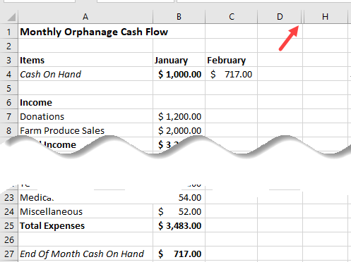
Suppose we have the following Excel dataset on Sheet1 of the workbook.

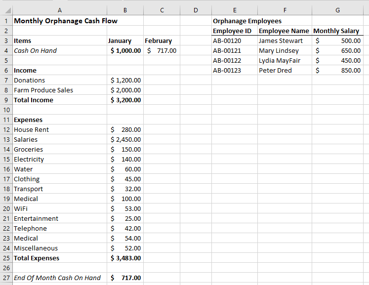
We want to use Excel VBA to hide columns E, F, and G, which contain employee data before we print the spreadsheet or send it out by email.

We use the following steps:

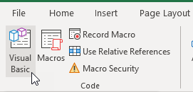
Click Developer >> Code >> Visual Basic to open the Visual Basic Editor.

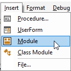
In the Visual Basic Editor, click Insert >> Module to create a new module.

Type the following procedure in the module.

Sub HideColumns()

Worksheets(«Sheet1»).Range(«E:G»).EntireColumn.Hidden = True

End Sub

Save the procedure and save the workbook as a Macro-Enabled Workbook. This ensures that the procedure is retained in the workbook for future use.
Click inside the procedure and press F5 to run the code.
Click the View Microsoft Excel button on the toolbar.

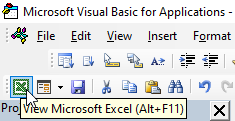
You are taken back to the active worksheet containing the dataset. Notice that columns E, F, and G are hidden.

Note: If you want to hide several non-contiguous columns, separate the column references by commas. For example, to hide columns E and G, we use the following sub-procedure:

Sub HideColumns()

Worksheets(«Sheet1»).Range(«E:E, G:G»).EntireColumn.Hidden = True

End Sub

Method #2: Excel VBA to Hide Columns Based on Cell Values

Suppose we have the following Excel dataset on Sheet2 of the workbook.

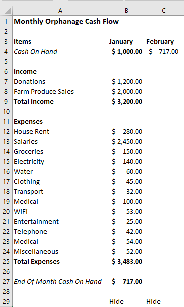
We want to use Excel VBA to hide the columns that have the word “Hide” in cells B29 and C29.

We use the steps below:

Click Developer >> Code >> Visual Basic to open the Visual Basic Editor.
In the Visual Basic Editor, click Insert >> Module to create a new module.
Type the following procedure in the module:

Sub HideColumnsOnCellValues()

Dim cell As Range

For Each cell In ActiveWorkbook.ActiveSheet.Rows(«29»).Cells

If cell.Value = «Hide» Then

cell.EntireColumn.Hidden = TRUE

End If

Next cell

End Sub

Place the cursor anywhere in the procedure and press F5 to run the code.

Click the View Microsoft Excel button on the toolbar to switch to the active workbook that contains the dataset. Notice that columns B and C that have the word “Hide” in cells B29 and B30 respectively are hidden.

How to Hide Rows Using Excel VBA

Method #1: Excel VBA Procedure to Hide Rows

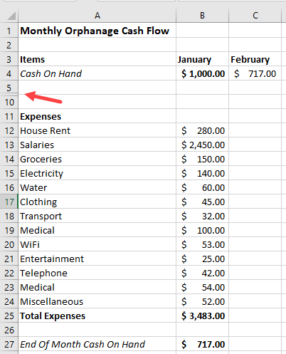
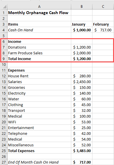
Suppose we have the following Excel dataset on Sheet1 of the workbook.

We want to hide rows 6, 7, 8, and 9, which contain data on the orphanage income before we print the spreadsheet or send it out by email.

We use the following steps:

Click Developer >> Code >> Visual Basic to open the Visual Basic Editor.

In the Visual Basic Editor, click Insert >> Module to create a new module.
Type the following procedure in the module:

Sub HideRows()

Worksheets(«Sheet1»).Range(«6:9»).EntireRow.Hidden = True

End Sub

Click inside the procedure and press F5 to run the code.
Click the View Microsoft Excel button on the toolbar. You are taken back to the active worksheet. Notice that rows 6, 7, 8, and 9 are hidden.

Note: If you want to hide several non-contiguous rows, separate the row references by commas. For example, to hide rows 6 and 8, we use the following sub-procedure:

Sub HideRows()

Worksheets(«Sheet1»).Range(«6:6, 8:8»).EntireRow.Hidden = True

End Sub

Method #2: Excel VBA to Hide Rows Based on Cell Values

Suppose we have the following Excel dataset on Sheet3 of the workbook.

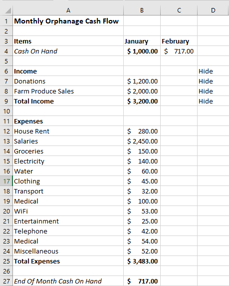
We want to use Excel VBA to hide all the rows that have the word “Hide” in column D.

We use the steps below:

Click Developer >> Code >> Visual Basic to open the Visual Basic Editor.
In the Visual Basic Editor, click Insert >> Module to create a new module.

Type the following procedure in the module:

Sub HideRowsOnCellValues()

Dim cell As Range

For Each cell In ActiveWorkbook.ActiveSheet.Columns(«D»).Cells

If cell.Value = «Hide» Then

cell.EntireRow.Hidden = TRUE

End If

Next cell

End Sub

Place the cursor anywhere in the procedure and press F5 to run the code.

Click the View Microsoft Excel button on the toolbar to switch back to the active worksheet containing the dataset. Notice that rows 6, 7, 8, and 9 that have the word “Hide” in cells D6, D7, D8, and D9, respectively, are hidden.

How to Unhide Columns Using Excel VBA

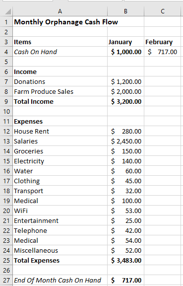
Suppose we have the following dataset on Sheet4 whose columns B and C are hidden.

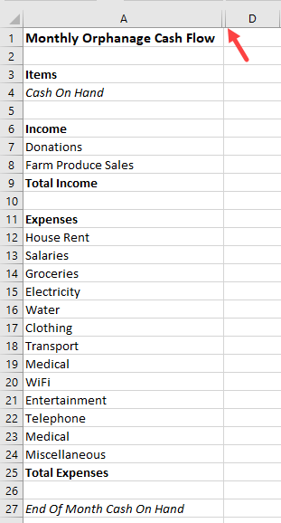
We want to unhide the two columns using an Excel VBA sub-procedure.

We use the following steps:

Click Developer >> Code >> Visual Basic to open the Visual Basic Editor.
In the Visual Basic Editor, click Insert >> Module to create a new module.
Type the following procedure in the module:

Sub UnhideColumns()

Worksheets(«Sheet4»).Range(«B:C»).EntireColumn.Hidden = False

End Sub

Click inside the sub-procedure and press F5 to run the code.

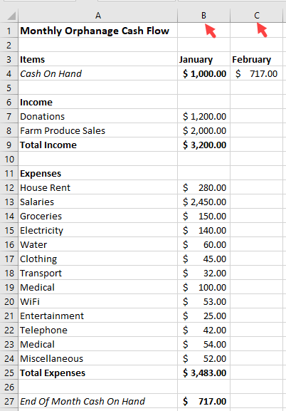
Click View Microsoft Excel on the toolbar to switch back to the active worksheet containing the dataset. Notice that columns B and C are unhidden.

How to Unhide Rows Using Excel VBA

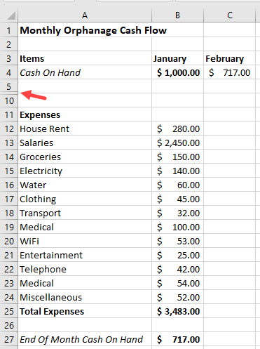
Suppose we have the following dataset whose rows 6, 7, 8, and 9 are hidden. The dataset is on Sheet5.

We want to unhide the four rows using Excel VBA.

We use the following steps:

Click Developer >> Code >> Visual Basic to open the Visual Basic Editor.

In the Visual Basic Editor, click Insert >> Module to create a new module.
Type the following procedure in the module:

Sub UnhideRows()

Worksheets(«Sheet5»).Range(«6:9»).EntireRow.Hidden = False

End Sub

Click inside the sub-procedure and press F5 to run the code.
Click View Microsoft Excel on the toolbar to switch back to the active worksheet containing the dataset. Notice that rows 6, 7, 8, and 9 are unhidden.

Conclusion

This tutorial has looked at how to hide or unhide columns and rows using Excel VBA. We hope you found the information helpful.

Post Views: 31

Источник

Working with large datasets that contain rows after rows of data can be quite painful.

In such cases, looking for data that match particular criteria can be like looking for a needle in a haystack.

Thankfully, Excel provides some features that let you hide certain rows based on the cell value so that you only see the rows that you want to see. There are two ways to do this:

Using filters
Using VBA

In this tutorial, we will discuss both methods, and you can pick the method you feel most comfortable with.

Using Filters to Hide Rows based on Cell Value

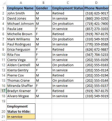
Let us say you have the dataset shown below, and you want to see data about only those employees who are still in service.

This is really easy to do using filters. Here are the steps you need to follow:

Select the working area of your dataset.
From the Data tab, select the Filter button. You will find it in the ‘Sort and Filter’ group.
You should now see a small arrow button on every cell of the header row.
These buttons are meant to help you filter your cells. You can click on any arrow to choose a filter for the corresponding column.
In this example, we want to filter out the rows that contain the Employment status = “In service”. So, select the arrow next to the Employment Status header.
Uncheck the boxes next to all the statuses, except “In service”. You can simply uncheck “Select All” to quickly uncheck everything and then just select “In service”.
Click OK.

You should now be able to see only the rows with Employment Status=”In service”. All other rows should now be hidden.

Note: To unhide the hidden cells, simply click on the Filter button again.

Using VBA to Hide Rows based on Cell Value

The second method requires a little coding. If you are accustomed to using macros and a little coding using VBA, then you get much more scope and flexibility to manipulate your data to behave exactly the way you want.

Writing the VBA Code

The following code will help you display only the rows that contain information about employees who are ‘In service’ and will hide all other rows:

Sub HideRows()
StartRow = 2
EndRow = 19
ColNum = 3
For i = StartRow To EndRow
If Cells(i, ColNum).Value <> "In service" Then
Cells(i, ColNum).EntireRow.Hidden = True
Else
Cells(i, ColNum).EntireRow.Hidden = False
End If
Next i
End Sub

The macro loops through each cell of column C and hide the rows that do not contain the value “In service”. It should essentially analyze each cell from rows 2 to 19 and adjust the ‘Hidden’ attribute of the row that you want to hide.

To enter the above code, copy it and paste it into your developer window. Here’s how:

From the Developer menu ribbon, select Visual Basic.
Once your VBA window opens, you will see all your files and folders in the Project Explorer on the left side. If you don’t see Project Explorer, click on View->Project Explorer.
Make sure ‘ThisWorkbook’ is selected under the VBA project with the same name as your Excel workbook.
Click Insert->Module. You should see a new module window open up.
Now you can start coding. Copy the above lines of code and paste them into the new module window.
In our example, we want to hide the rows that do not contain the value ‘In service’ in column 3. But you can replace the value of ColNum number from “3” in line 4 to the column number containing your criteria values.
Close the VBA window.

Note: If your dataset covers more than 19 rows, you can change the values of the StartRow and EndRow variables to your required row numbers.

If you can’t see the Developer ribbon, from the File menu, go to Options. Select Customize Ribbon and check the Developer option from Main Tabs.

Finally, Click OK.

Your macro is now ready to use.

Running the Macro

Whenever you need to use the above macro, all you need to do is run it, and here’s how:

Select the Developer tab
Click on the Macros button (under the Code group).
This will open the Macro Window, where you will find the names of all the macros that you have created so far.
Select the macro (or module) named ‘HideRows’ and click on the Run button.

You should see all the rows where Employment Status is not ’In service’ hidden.

Explanation of the Code

Here’s a line by line explanation of the above code:

In line 1 we defined the function name.

Sub HideRows()

In lines 2, 3 and 4 we defined variables to hold the starting row and ending row of the dataset as well as the index of the criteria column.

StartRow = 2
EndRow = 19
ColNum = 3

In lines 5 to 11, we looped through each cell in column “3” (or column C) of the Active Worksheet. If a cell does not contain the value “Inservice”, then we set the ‘Hidden’ attribute of the entire row (corresponding to that cell) to True, which means we want to hide the entire corresponding row.

For i = StartRow To EndRow
If Cells(i, ColNum).Value <> "In service" Then
Cells(i, ColNum).EntireRow.Hidden = True
Else
Cells(i, ColNum).EntireRow.Hidden = False
End If
Next i

Line 12 simply demarcates the end of the HideRows function.

End Sub

In this way, the above code hides all the rows that do not contain the value ‘In service’ in column C.

Un-hiding Columns Based On Cell Value

Now that we have been able to successfully hide unwanted rows, what if we want to see the hidden rows again?

Doing this is quite easy. You only need to make a small change to the HideRows function.

Sub UnhideRows()
StartRow = 2
EndRow = 19
ColNum = 3
For i = StartRow To EndRow
Cells(i, ColNum).EntireRow.Hidden = False
Next i
End Sub

Here, we simply ensured that irrespective of the value, all the rows are displayed (by setting the Hidden property of all rows to False).

You can run this macro in exactly the same way as HideRows.

Hiding Rows Based On Cell Values in Real-Time

In the first example, the columns are hidden only when the macro runs. However, most of the time, we want to hide columns on-the-fly, based on the value in a particular cell.

So, let’s now take a look at another example that demonstrates this. In this example, we have the following dataset:

The only difference from the first dataset is that we have a value in cell A21 that will determine which rows should be hidden. So when cell A21 contains the value ‘Retired’ then only the rows containing the Employment Status ‘Retired’ are hidden.

Similarly, when cell A21 contains the value ‘On probation’ then only the rows containing the Employment Status ‘On probation’ are hidden.

When there is nothing in cell A21, we want all rows to be displayed.

We want this to happen in real-time, every time the value in cell A21 changes. For this, we need to make use of Excel’s Worksheet_SelectionChange function.

The Worksheet_SelectionChange Event

The Worksheet_SelectionChange procedure is an Excel built-in VBA event

It comes pre-installed with the worksheet and is called whenever a user selects a cell and then changes his/her selection to some other cell.

Since this function comes pre-installed with the worksheet, you need to place it in the code module of the correct sheet so that you can use it.

In our code, we are going to put all our lines inside this function, so that they get executed whenever the user changes the value in A21 and then selects some other cell.

Writing the VBA Code

Here’s the code that we are going to use:

StartRow = 2
EndRow = 19
ColNum = 3
For i = StartRow To EndRow
If Cells(i, ColNum).Value = Range("A21").Value Then
Cells(i, ColNum).EntireRow.Hidden = True
Else
Cells(i, ColNum).EntireRow.Hidden = False
End If
Next i

To enter the above code, you need to copy it and paste it in your developer window, inside your worksheet’s Worksheet_SelectionChange procedure. Here’s how:

From the Developer menu ribbon, select Visual Basic.
Once your VBA window opens, you will see all your project files and folders in the Project Explorer on the left side.
In the Project Explorer, double click on the name of your worksheet, under the VBA project with the same name as your Excel workbook. In our example, we are working with Sheet1.
This will open up a new module window for your selected sheet.
Click on the dropdown arrow on the left of the window. You should see an option that says ‘Worksheet’.
Click on the ‘Worksheet’ option. By default, you will see the Worksheet_SelectionChange procedure created for you in the module window.
Now you can start coding. Copy the above lines of code and paste them into the Worksheet_SelectionChange procedure, right after the line: Private Sub Worksheet_SelectionChange(ByVal Target As Range).
Close the VBA window.

Running the Macro

The Worksheet_SelectionChange procedure starts running as soon as you are done coding. So you don’t need to explicitly run the macro for it to start working.

Try typing the ‘Retired’ in the cell A21, then clicking any other cell. You should find all rows containing the value ‘Retired’ in column C disappear.

Now try replacing the value in cell A21 to ‘On probation’, then clicking any other cell. You should find all rows containing the value ‘On probation’ in column C disappear.

Now try removing the value in cell A21 and leaving it empty. Then click on any other cell. You should find both rows become visible again.

This means the code is working in real-time when changes are made to cell B20.

Explanation of the Code

Let us take a few minutes to understand this code now.

Lines 1, 2, and 3 define variables to hold the starting row and ending row of the dataset as well as the index of the criteria column. You can change the values according to your requirement.

StartRow = 2
EndRow = 19
ColNum = 3

Lines 4 to 10, loop through each cell in column “3” (or column C) of the worksheet. If the cell contains the value in cell A21, then we set the ‘Hidden’ attribute of the entire row (corresponding to that cell) to True, which means we want to hide the entire corresponding row.

For i = StartRow To EndRow
If Cells(i, ColNum).Value = Range("A21").Value Then
Cells(i, ColNum).EntireRow.Hidden = True
Else
Cells(i, ColNum).EntireRow.Hidden = False
End If
Next i

In this way, the above code hides the rows of the dataset depending on the value in cell A21. If A21 does not contain any value then the code displays all rows.

In this tutorial, I showed you how you can use Filters as well as Excel VBA to hide rows based on a cell value.

I did this with the help of two simple examples – one that removes required rows only when the macro is explicitly run and another that works in real-time.

I hope that we have been successful in helping you understand the concept behind the code so that you can customize it and use it in your own applications.

Other Excel tutorials you may also like:

How to Hide Columns Based On Cell Value in Excel
How to Delete Filtered Rows in Excel (with and without VBA)
How to Highlight Every Other Row in Excel (Conditional Formatting & VBA)
How to Unhide All Rows in Excel with VBA
How to Set a Row to Print on Every Page in Excel
How to Paste in a Filtered Column Skipping the Hidden Cells
How to Select Multiple Rows in Excel
How to Select Rows with Specific Text in Excel
How to Move Row to Another Sheet Based On Cell Value in Excel?
How to Compare Two Cells in Excel?

Источник

I am trying to hide all rows containing the value «xx» in column A and not hide the rows containing «a» in column A. The range is from A8:A556. This macro needs to be triggered by a change in cell C4.

Any idea why it is not working? Here’s the current attempt:

Private Sub Worksheet_Change(ByVal Target As Range)

If Target.Address(True, True) = "$C$4" Then

    If Range("A8:A555").Value = "xx" Then
        Rows("8:555").EntireRow.Hidden = True
    ElseIf Range("A8:A555").Value = "a" Then
        Rows("8:555").EntireRow.Hidden = False

     End If
   End If

End Sub

Thanks!

EDIT:

Hey Fixer1234, Here is the detail:

«xx» and «a» may not exist together if the macro works correctly.
Only «xx» rows must be hidden
«xx» values are not in combination with values that cannot be hidden.
«a» values are not in combination with values that must be hidden.
there are other rows that do not contain «xx or «a» that don’t need to be hidden (should I add an «a» to these columns or completely remove the IfElse?).
«xx» row contain other formulas, a blank result from the formula means the row must be hidden.
«a» rows have the same formula but it produces a result and must not be hidden.

Run-time error ’13’: type mismatch
and then the debug goes to the first
If Range("A8:A555").Value = "xx" Then

asked Apr 4, 2019 at 1:03

KaitwaKaitwa

211 gold badge1 silver badge3 bronze badges

You can’t test all the values in a range using Range("A8:A555").Value = "xx". It will throw a Type Mismatch error.

You need to loop through each cell in the range and test individually if its Value equals «xx».

To make the code run faster, don’t hide rows as you detect them but build up a Range of Ranges to be hidden then hide them all at once.

Private Sub Worksheet_SelectionChange(ByVal Target As Range)
Dim cel As Range
Dim RangeToHide As Range

    'Test if Target is C4
    If Not Intersect(Target, [C4]) Is Nothing Then
        'Loop through each cell in range and test if it's "xx"
        For Each cel In Range("A8:A555")
            If cel = "xx" Then
                If RangeToHide Is Nothing Then
                    'Initialise RangeToHide because Union requires at least 2 ranges
                    Set RangeToHide = cel
                Else
                    'Add cel to RangeToHide
                    Set RangeToHide = Union(RangeToHide, cel)
                End If
            End If
        Next
        RangeToHide.EntireRow.Hidden = True
    End If
End Sub

answered Apr 4, 2019 at 6:18

Mark FitzgeraldMark Fitzgerald

5221 gold badge3 silver badges11 bronze badges

Use this VBA code as Standard Module, will help you to Hide all rows having either XX or xx in Column A.

Private Sub Worksheet_Change(ByVal Target As Range)

If Target.Address(True, True) = "$C$4" Then

Dim i As Integer
  Application.ScreenUpdating = False



    For i = 8 To 255

    If Sheets("Sheet1").Range("A" & i).Value = "XX" Or Sheets("Sheet1").Range("A" & i).Value = "xx" Then
    Rows(i & ":" & i).EntireRow.Hidden = True
    End If


    Next i
    End If

    Application.ScreenUpdating = True


End Sub

N.B.

No need to use any code to Unhide rows having a or A, since already are Visible. And above all the used code is hiding specific Rows in Column A.

answered Apr 4, 2019 at 5:53

Rajesh SinhaRajesh Sinha

8,8926 gold badges15 silver badges35 bronze badges

How do I hide separate rows!?
This is how I think:

Private Sub CheckBox1_Click()
If CheckBox1 = False Then
    [15:15].EntireRow.Hidden = True
    [3:3].EntireRow.Hidden = True
Else
    [15:15].EntireRow.Hidden = False
    [3:3].EntireRow.Hidden = False
End If

Best Regards
Mattias

zx485

2,17011 gold badges17 silver badges23 bronze badges

answered May 1, 2020 at 14:26

Источник

Home / VBA / Excel VBA Hide and Unhide a Column or a Row

VBA Hidden Property

To hide/unhide a column or a row in Excel using VBA, you can use the “Hidden” property. To use this property, you need to specify the column, or the row using the range object and then specify the TRUE/FALSE.

Specify the column or the row using the range object.
After that, use the entire column/row property to refer to the entire row or column.
Next, use the hidden property.
In the end, specify the true/false.

Following is the example to consider:

Sub vba_hide_row_columns()
'hide the column A
Range("A:A").EntireColumn.Hidden = True
'hide the row 1
Range("1:1").EntireRow.Hidden = True
End Sub

In the above code, we have used the hidden property to hide columns A and row 1. And here is the code for unhiding them back.

Sub vba_hide_row_columns()
'unhide the column A
Range("A:A").EntireColumn.Hidden = False
'unhide the row 1
Range("1:1").EnitreRow.Hidden = False
End Sub

VBA Hide/Unhide Multiple Rows and Columns

Sub vba_hide_row_columns()
'hide the column A to c
Range("A:C").EntireColumn.Hidden = True
'hide the row 1 to 4
Range("1:4").EntireRow.Hidden = True
End Sub

And in the same way, if you want to unhide multiple rows and columns.

Sub vba_hide_row_columns()
'hide the column A to c
Range("A:C").EntireColumn.Hidden = False
'hide the row 1 to 4
Range("1:4").EntireRow.Hidden = False
End Sub

Hide All Columns and Rows

Sub vba_hide_row_columns()

'hide the column A
Columns.EntireColumn.Hidden = True

'hide the row 1
Rows.EntireRow.Hidden = True

End Sub

Unhide All Columns and Rows

Sub vba_hide_row_columns()

'unhide all the columns
Columns.EntireColumn.Hidden = False

'unhide all the rows
Rows.EntireRow.Hidden = False

End Sub

Hide/Unhide Columns and Rows in Another Worksheet

Sub vba_hide_row_columns()

'hide all columns in the sheet 1
Worksheets("Sheet1").Columns.EntireColumn.Hidden = False

'hide all rows in the sheet 1
Worksheets("Sheet1").Rows.EntireRow.Hidden = False

End Sub

Excel VBA Constructs To Hide Rows Or Columns

Hide Or Unhide With The Range.Hidden Property

How To Hide Rows Or Columns With The Range.Hidden Property

How To Unhide Rows Or Columns With The Range.Hidden Property

Specify Row Or Column To Hide Or Unhide Using VBA

Worksheet.Range Property

Syntax #1: expression.Range(Cell)

Syntax #2: expression.Range(Cell1, Cell2)

How To Refer To An Entire Row Or Column With the Worksheet.Range Property

Worksheet.Cells Property

Worksheet.Columns Property

Worksheet.Rows Property

Range.EntireRow Property

Range.EntireColumn Property

VBA Code Example #1: Hide A Column

VBA Code Example #2: Hide Several Contiguous Columns

VBA Code Example #3: Hide Several Non-Contiguous Columns

Excel VBA Code Examples To Hide Rows

VBA Code Example #4: Hide A Row

VBA Code Example #5: Hide Several Contiguous Rows

VBA Code Example #6: Hide Several Non-Contiguous Rows

Excel VBA Code Examples To Unhide Columns

VBA Code Example #7: Unhide A Column

VBA Code Example #8: Unhide Several Contiguous Columns

VBA Code Example #9: Unhide Several Non-Contiguous Columns

VBA Code Examples #10 And #11: Unhide All Columns In A Worksheet

VBA Code Example #10: Unhide All Columns In A Worksheet Using The Worksheet.Cells Property

VBA Code Example #11: Unhide All Columns In A Worksheet Using The Worksheet.Columns Property

Excel VBA Code Examples To Unhide Rows

VBA Code Example #12: Unhide A Row

VBA Code Example #13: Unhide Several Contiguous Rows

VBA Code Example #14: Unhide Several Non-Contiguous Rows

VBA Code Examples #15 And #16: Unhide All Columns In A Worksheet

VBA Code Example #15: Unhide All Rows In A Worksheet Using The Worksheet.Cells Property

VBA Code Example #16: Unhide All Rows In A Worksheet Using The Worksheet.Rows Property

Conclusion

Books Referenced In This Excel VBA Tutorial

Hide Columns or Rows

Hide Columns

Hide Rows

Unhide Columns or Rows

Unhide All Columns or Rows

VBA Coding Made Easy

Синтаксис

Примечание

Примеры кода с Range.Hidden

Пример 1

Пример 2

Пример 3

Пример 4

Hide UnHide Rows in Excel Worksheet using VBA

17 Comments

Project Management

Excel VBA

Method #1: Excel VBA Procedure to Hide Columns

Method #2: Excel VBA to Hide Columns Based on Cell Values

How to Hide Rows Using Excel VBA

Method #1: Excel VBA Procedure to Hide Rows

Method #2: Excel VBA to Hide Rows Based on Cell Values

How to Unhide Columns Using Excel VBA

How to Unhide Rows Using Excel VBA

Conclusion

Using Filters to Hide Rows based on Cell Value

Using VBA to Hide Rows based on Cell Value

Writing the VBA Code

Running the Macro

Explanation of the Code

Un-hiding Columns Based On Cell Value

Hiding Rows Based On Cell Values in Real-Time

The Worksheet_SelectionChange Event

Writing the VBA Code

Running the Macro

Explanation of the Code

VBA Hidden Property

VBA Hide/Unhide Multiple Rows and Columns

Hide All Columns and Rows

Unhide All Columns and Rows

Hide/Unhide Columns and Rows in Another Worksheet

More Tutorials