
Hide or show rows or columns
Hide or unhide columns in your spreadsheet to show just the data that you need to see or print.

Hide columns
-
Select one or more columns, and then press Ctrl to select additional columns that aren’t adjacent.
-
Right-click the selected columns, and then select Hide.
Note: The double line between two columns is an indicator that you’ve hidden a column.
Unhide columns
-
Select the adjacent columns for the hidden columns.
-
Right-click the selected columns, and then select Unhide.
Or double-click the double line between the two columns where hidden columns exist.
Need more help?
You can always ask an expert in the Excel Tech Community or get support in the Answers community.
See Also
Unhide the first column or row in a worksheet
Need more help?
Want more options?
Explore subscription benefits, browse training courses, learn how to secure your device, and more.
Communities help you ask and answer questions, give feedback, and hear from experts with rich knowledge.
Hiding Excel Column(s)
Hiding a column in excel implies making it invisible so that it is removed from display. A hidden column is not deleted from the worksheet. This means that it does exist and has been only temporarily held from view. In Excel, one can hide both contiguous and non-contiguous columns. However, to use a hidden column again, it needs to be unhidden at first.
For example, a column containing calculations may be hidden. This helps avoid confusion amongst users of a shared worksheet.
A column is hidden when its data needs to be concealed from other Excel users, it is unused and not required for a while, its presence is making comparisons between the remaining columns difficult, and so on. The purpose of hiding an excel column is to allow viewing the relevant areas of a worksheet at a given time.
Table of contents
- Hiding Excel Column(s)
- How to Hide Columns in Excel? (Top 4 Methods)
- Example #1–Hide Columns Using the “Hide” Option of the Context Menu
- Example #2–Hide Excel Columns Using the “Ctrl+Zero (0)” Shortcut
- Example #3–Hide Excel Columns by Setting the Column Width as Zero
- Example #4–Hide Columns Using VBA Code
- Frequently Asked Questions
- Recommended Articles
- How to Hide Columns in Excel? (Top 4 Methods)
How to Hide Columns in Excel? (Top 4 Methods)
The techniques of hiding columns in Excel are listed as follows:
- “Hide” option of the context menu
- “Ctrl+zero (0)” shortcut
- Column width as zero
- VBA code
Let us discuss these methods one by one with the help of examples.
Note: All the following examples demonstrate the process of hiding adjacent (contiguous) columns. For hiding multiple non-adjacent columns, refer to the second question under the heading “frequently asked questions.” This is given at the end of this article.
Example #1–Hide Columns Using the “Hide” Option of the Context Menu
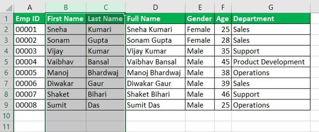
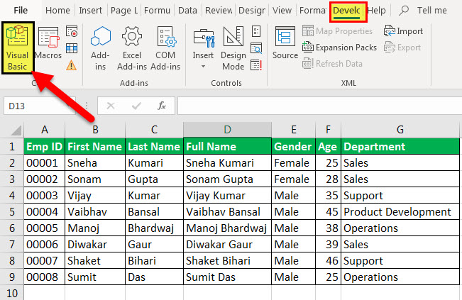
The following table displays the IDs, names, gender, age, and department of some employees of an organization. Consider one column of the table as one column of an Excel worksheet. So, the dataset begins from column A (emp ID) and ends with column G (department).
The first name (column B) and last name (column C) have been concatenated (joined) to form the full name (column D). Since columns B and C are not required (for some time), we want to hide them using the “hide” option of the context menu.
| Emp ID | First Name | Last Name | Full Name | Gender | Age | Department |
|---|---|---|---|---|---|---|
| 00001 | Sneha | Kumari | Sneha Kumari | Female | 25 | Sales |
| 00002 | Sonam | Gupta | Sonam Gupta | Female | 28 | Sales |
| 00003 | Vijay | Kumar | Vijay Kumar | Male | 35 | Support |
| 00004 | Vaibhav | Bansal | Vaibhav Bansal | Male | 45 | Product Development |
| 00005 | Manoj | Bhardwaj | Manoj Bhardwaj | Male | 38 | Operations |
| 00006 | Diwakar | Gaur | Diwakar Gaur | Male | 39 | Sales |
| 00007 | Shaket | Bihari | Shaket Bihari | Male | 46 | Support |
| 00008 | Sumit | Das | Sumit Das | Male | 25 | Operations |
The steps to hide excel columns is listed as follows:
- With the help of the mouse, click the label of column B appearing on top. This selects column B entirely. Next, press the keys “Shift+right arrow” to select the entire column C.
The selection is shown in the succeeding image. Notice that in column A, the numbers have been formatted as text. This has been done to place zeros before each number in cells A2 to A9.
Note 1: For “Shift+right arrow” to work, hold the “Shift” key, and at the same time, press the right arrow. When the shortcut “Shift+right arrow” is pressed after selecting a column, the selection is extended to an adjacent column on the right.
When the shortcut “Shift+right arrow” is pressed after selecting a cell, the selection is extended to an adjacent cell on the right.
Note 2: When the numbers of column A were formatted as text, green triangles (shown in the first image of example #2) had appeared on the upper-left corner of each cell. From the “trace error” button, we clicked “ignore error” (for each cell) to remove such green triangles.

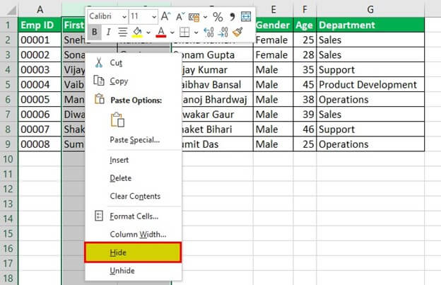
- Right-click the selection and choose “hide” from the context menu. The same is shown in the following image.

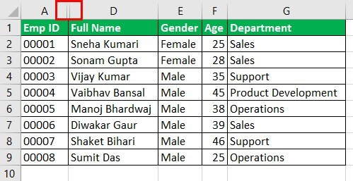
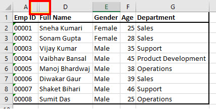
- The final dataset, with columns B and C hidden, is shown in the following image. Notice that there are double vertical lines (shown in a red box) between the column labels A and D. These lines indicate that columns B and C have been hidden.
Another indication of hidden excel columns is the change in the sequence of the column labels. After label A, labels B and C are skipped, and straightaway label D is displayed.

Example #2–Hide Excel Columns Using the “Ctrl+Zero (0)” Shortcut
The following image shows a dataset similar to that of example #1. Notice that the number of columns has been reduced this time. Columns A to D are displayed, which consist of the employee ID, first name, last name, and full name respectively.
Ignore the green triangles in column A of the subsequent images. These are displayed because the “ignore error” option from the “trace error” button has not been clicked, unlike in step 1 of the preceding example (example #1).
We want to hide columns B and C by using the shortcut “Ctrl+zero (0)” in Excel.

The steps to hide the stated columns using the given technique are listed as follows:
Step 1: Select columns B and C, which need to be hidden. For this, click the label of column B with the mouse and drag it across to column C. When the mouse pointer is placed on the label of column B, it changes to an arrow pointing downwards.
Note: Alternatively, select any cell of column B and press the keys “Ctrl+space” together. Column B is selected entirely. Next, press the keys “Shift+right arrow” to select column C.
Step 2: Once the columns to be hidden (columns B and C) are selected, press the keys “Ctrl+zero (0)” together.
The steps 1 and 2 are shown in the following image. Hence, columns B and C (selected in step 1) are hidden. Notice that, in the final output, the double vertical lines separate the labels of columns A and D.
Example #3–Hide Excel Columns by Setting the Column Width as Zero
Working on the dataset of example #2, we want to hide columns B and C by setting the column widthA user can set the width of a column in an excel worksheet between 0 and 255, where one character width equals one unit. The column width for a new excel sheet is 8.43 characters, which is equal to 64 pixels.read more as zero.
The steps to hide the mentioned columns using the given technique are listed as follows:
Step 1: Select the columns to be hidden. So, select columns B and C entirely.
Step 2: Right-click the selection and choose “column width” from the context menu. Set column width as zero and click “Ok.”
Both steps 1 and 2 are shown in the following image. The final dataset, with columns B and C hidden, is also displayed in this image. Double vertical lines appear between the labels of columns A and D.
Note: When a column’s width is entered as zero, the column is hidden from the worksheet.
Example #4–Hide Columns Using VBA Code
Working on the dataset of example #1, we want to hide columns B and C with the help of a VBA codeVBA code refers to a set of instructions written by the user in the Visual Basic Applications programming language on a Visual Basic Editor (VBE) to perform a specific task.read more. Consider the dataset to be in “sheet1” of Excel.
The steps to hide columns using a VBA code are listed as follows:
Step 1: From the Developer tab, click “visual basic.” This is shown in the following image.
Note: If the Developer tabEnabling the developer tab in excel can help the user perform various functions for VBA, Macros and Add-ins like importing and exporting XML, designing forms, etc. This tab is disabled by default on excel; thus, the user needs to enable it first from the options menu.read more is not displayed on the ribbon, it must be enabled from the File tab. For the detailed steps, click the given hyperlink.
Step 2: A new window titled “Microsoft visual basic for applications” opens. Double-click “sheet1.” Next, from the Insert tab, click “procedure.” Specify the name of the procedure and paste the following code:
Worksheets(“Sheet1”).Columns(“B:C”).Hidden = True
This is shown in the following image.

Step 3: Save the file with the .xlsm extension as it supports macros. This extension is used for a macro-enabled workbook, which has been created in Excel 2007 or the newer Excel versions.
Step 4: From the Run tab, click “run sub/user form.” The output is shown in the following image. Notice the double line (shown in a red box) between the column labels A and D. This indicates that the columns in between (i.e., columns B and C) are hidden.
Frequently Asked Questions
1. What does it mean to hide columns and how is it done in Excel?
To hide a column means removing one or more excel columns from the display. Such hidden columns do exist in the worksheet even though they become invisible. Columns are usually hidden when they are neither being used nor meant to be deleted.
The steps to hide a column in Excel are listed as follows:
a. Select the column to be hidden.
b. Right-click the selection and choose “hide” from the context menu.
The column selected in step “a” is hidden.
Note: For more techniques of hiding a column, refer to the examples of this article.
2. How to hide multiple columns in Excel?
The steps to hide multiple columns in Excel are listed as follows:
a. Select all the columns that need to be hidden.
• For selecting multiple contiguous columns, drag across the column labels with the mouse. Alternatively, select the first column and press the keys “Shift+right arrow” to select columns on the right.
• For selecting multiple non-contiguous columns, click the first column label. Thereafter, hold the “Ctrl” key and click the other column labels.
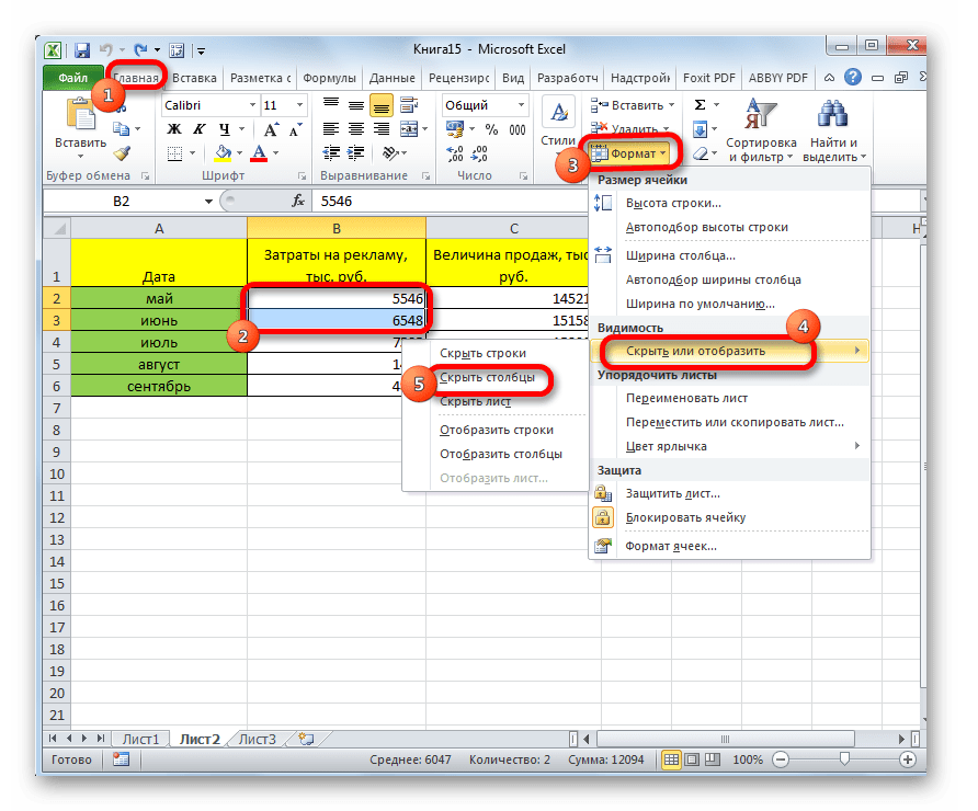
b. From the Home tab, click the “format” drop-down in the “cells” group.
c. Under “visibility,” select “hide & unhide.” Next, choose “hide columns.”
The columns selected in step “a” are hidden.
3. How to hide and lock columns in Excel?
The steps to hide and lock columns in Excel are listed as follows:
a. Select the entire worksheet by pressing either the keys “Ctrl+A” or the “select all” button. The “select all” button is located at the top-left corner of the Excel worksheet.
b. Right-click the selection and choose “format cells” from the context menu. The “format cells” dialog box opens. Uncheck the “locked” option in the “protection” tab. Click “Ok.”
c. Select the columns to be hidden and locked. Open the “format cells” dialog box again and click the “protection” tab. Check the “locked” option and click “Ok.”
d. Hide the columns selected in the preceding step (step c). For this, keep the columns to be hidden selected and click the “format” drop-down from the Home tab. Next, click “hide columns” from the “hide & unhide” option.
e. From the Review tab, click “protect sheet.” The “protect sheet” dialog box opens. Keep the following checkboxes selected:
• “Protect worksheet and contents of locked cell”
• “Select locked cells”
• “Select unlocked cells”
f. Enter a password and confirm it. Click “Ok” to proceed. The “protect sheet” dialog box closes.
The columns selected in step “c” are hidden. Since the worksheet is protected, these hidden columns cannot be unhidden by the usual ways to unhide a column. The advantage of locking hidden columns is that their content is concealed from the other users of the worksheet.
Note: To unhide the hidden columns, unprotect the sheet in the first place. To unprotect the sheet, click “unprotect sheet” from the Review tab. Next, enter the password and click “Ok.”
Thereafter, unhide the columns by selecting, right-clicking, and choosing “unhide” from the context menu. Alternatively, select the columns and choose “unhide columns” from the “hide & unhide” option of the “format” drop-down (in the Home tab).
Recommended Articles
This has been a guide to hiding columns in excel. Here we discuss the top 4 methods to hide columns in Excel, including the “hide” option of the context menu, shortcut (Ctrl+0), column width (as zero), and VBA code. You can learn more about Excel from the following articles –
- VBA Hide Columns
- Excel Hide Shortcut
- How to Unhide Columns in Excel?
- How to Freeze or Lock Multiple Columns in Excel?
- FLOOR Function in Excel
![]()
Download Article
![]()
Download Article
Want to hide certain columns in your spreadsheet? Hiding columns in Excel is a great way to get a better look at your data, especially when printing. We’ll show you how to hide columns in a Microsoft Excel spreadsheet, as well as how to show columns that you’ve hidden.
Steps
-

1
Double-click your spreadsheet to open it in Excel.
- If Excel is already open, you can open your spreadsheet by pressing Ctrl + O (Windows) or Cmd + O (macOS) and then selecting the file.
-
2
Click the letter above the column you want to hide. This selects the entire column.
- For example, to select the first column (column A), click the A at the top of the column.
- If you want to hide multiple columns at once, just click and drag your cursor over the column letters you want to hide.
- You can also select multiple non-adjacent columns by holding down Ctrl as you click each column letter.
Advertisement
-
3
Right-click the selected column(s). This brings up a menu.
- If you don’t have multiple mouse buttons, hold down the Ctrl key as you click the column(s) instead.
-
4
Click Hide on the menu. Any selected columns are now hidden.[1]
-
5
Unhide columns (optional). If you want to show columns that are hidden, just click any column adjacent to those hidden to select it, and then choose Unhide.


Advertisement
Ask a Question
200 characters left
Include your email address to get a message when this question is answered.
Submit
Advertisement
Thanks for submitting a tip for review!
References
About This Article
Article SummaryX
1. Open your spreadsheet.
2. Select the column(s) you want to hide.
3. Right-click the selected column(s).
4. Click Hide.
Did this summary help you?
Thanks to all authors for creating a page that has been read 42,783 times.
Is this article up to date?
Hide and Unhide Rows and Columns in Microsoft Excel (with Shortcuts)
by Avantix Learning Team | Updated January 29, 2022
Applies to: Microsoft® Excel® 2013, 2016, 2019 and 365 (Windows)
You can hide or unhide columns or rows in Excel using the context menu, using a keyboard shortcut or by using the Format command on the Home tab in the Ribbon. You can quickly unhide all columns or rows as well.
Some users may want to hide all of the unused columns to the right and unused rows below the data to clean up the workspace and display only relevant information to team members or clients.
You will not be able to hide or unhide rows or columns if the worksheet has been protected with a password (and you don’t have the password to unprotect it), if content has been disabled or if the file is read only.
Recommended article: How to Lock and Protect Excel Worksheets and Workbooks
Selecting columns or rows in Excel
It’s important to be able to quickly select columns or rows in Excel if you want to hide them.
To select one or more columns in Excel:
- To select one column, click its heading or select a cell in the column and press Ctrl + spacebar.
- To select multiple contiguous columns, drag across the column headings using a mouse or select the first column and then Shift-click the last column.
- To select non-contiguous columns, click the heading of the first column and then Ctrl-click the headings or the other columns you want to select.
To select one or more rows in Excel:
- To select one row, click its heading or select a cell in the row and press Shift + Spacebar.
- To select multiple contiguous rows, drag across the row headings using a mouse or select the first row and then Shift-click the last row.
- To select non-contiguous rows, click the heading of the first row and then Ctrl-click the headings of the other rows you want to select.
To select all rows and columns in Excel:
- Press Ctrl + A (press A twice if necessary).
- Click in the intersection box to the left of the A and above the 1 on the worksheet.
Hiding columns
To hide a column or columns by right-clicking:
- Select the column or columns you want to hide.
- Right-click and select Hide from the drop-down menu.
To hide a column or columns using a keyboard shortcut:
- Select the column or columns you want to hide.
- Press Ctrl + 0 (zero).
To hide a column or columns using the Ribbon:
- Select the column or columns you want to hide.
- Click the Home tab in the Ribbon.
- In the Cells group, click Format. A drop-down menu appears.
- Click Visibility, select Hide & Unhide and then Hide Columns.
To hide all columns to the right of the last line of data:
- Select the column to the right of the last column of data.
- Press Ctrl + Shift + right arrow.
- Press Ctrl + 0 (zero). You can also use the Ribbon method or the right-click method to hide columns.
Unhiding columns
To unhide a column or columns by right-clicking:
- Select the column headings to the left and right of the hidden column(s). To unhide all columns, click the box to the left of the A and above the 1 on the worksheet or press Ctrl + A (twice if necessary).
- Right-click and select Unhide from the drop-down menu.
To unhide a column or columns using a keyboard shortcut:
- Select the column headings to the left and right of the hidden column(s) by dragging. To unhide all columns, click the box to the left of the A and above the 1 on the worksheet or press Ctrl + A (twice if necessary).
- Press Ctrl + Shift + 0 (zero). If this doesn’t work, use one of the other methods.
To unhide a column or columns using the Ribbon:
- Select the column headings to the left and right of the hidden column(s). To select all columns, click the box to the left of the A and above the 1 on the worksheet or press Ctrl + A (twice if necessary).
- Click the Home tab in the Ribbon.
- In the Cells group, click Format. A drop-down menu appears.
- Click Visibility, select Hide & Unhide and then Unhide Columns.
To unhide a column or columns by double-clicking:
- Select the column headings to the left and right of the hidden columns(s).
- Hover the mouse over the hidden column headings.
- When the mouse pointer turns into a split two-headed arrow, double-click.
Hiding rows
To hide a row or rows by right-clicking:
- Select the row or rows you want to hide.
- Right-click and select Hide from the drop-down menu.
To hide a row or rows using a keyboard shortcut:
- Select the row or rows you want to hide.
- Press Ctrl + 9.
To hide a row or rows using the Ribbon:
- Select the row or rows you want to hide.
- Click the Home tab in the Ribbon.
- In the Cells group, click Format. A drop-down menu appears.
- Click Visibility, select Hide & Unhide and then Hide Rows.
To hide all rows below the last line of data:
- Select the row below the last line of data.
- Press Ctrl + Shift + down arrow.
- Press Ctrl + 9. You can also use the Ribbon method or the right-click method to hide the rows.
Unhiding rows
To unhide a row or rows by right-clicking:
- Select the row headings above and below the hidden row(s). To unhide all rows, click the box to the left of the A and above the 1 on the worksheet.
- Right-click and select Unhide from the drop-down menu.
To unhide rows using a keyboard shortcut:
- Select the row headings above and below the hidden row(s). To unhide all rows, click the box to the left of the A and above the 1 on the worksheet or press Ctrl + A (twice if necessary).
- Press Ctrl + Shift + 9.
To unhide a row or rows using the Ribbon:
- Select the row headings above and below the hidden row(s). To select all rows, click the box to the left of the A and above the 1 on the worksheet.
- Click the Home tab in the Ribbon or press Ctrl + A (twice if necessary).
- In the Cells group, click Format. A drop-down menu appears.
- Click Visibility, select Hide & Unhide and then Unhide Rows.
To unhide a row or rows by double-clicking:
- Select the row headings above and below the hidden row(s). To unhide all rows, click the box to the left of the A and above the 1 on the worksheet.
- Hover the mouse over the hidden row headings.
- When the mouse pointer turns into a split two-headed arrow, double-click.
The method you use to hide or unhide columns or rows is based on personal preference.
Subscribe to get more articles like this one
Did you find this article helpful? If you would like to receive new articles, join our email list.
More resources
How to Convert Text to Numbers in Excel (5 Ways)
How to Use Flash Fill in Excel (4 Ways with Shortcuts)
10 Ways to Save Time Selecting in Excel using the Name Box
How to Delete Blank Rows in Excel (5 Easy Ways with Shortcuts)
How to Highlight Errors, Blanks and Duplicates in Excel Worksheets (Using Formulas)
Related courses
Microsoft Excel: Intermediate / Advanced
Microsoft Excel: Data Analysis with Functions, Dashboards and What-If Analysis Tools
Microsoft Excel: Introduction to Visual Basic for Applications (VBA)
VIEW MORE COURSES >
Our instructor-led courses are delivered in virtual classroom format or at our downtown Toronto location at 18 King Street East, Suite 1400, Toronto, Ontario, Canada (some in-person classroom courses may also be delivered at an alternate downtown Toronto location). Contact us at info@avantixlearning.ca if you’d like to arrange custom instructor-led virtual classroom or onsite training on a date that’s convenient for you.
Copyright 2023 Avantix® Learning
Microsoft, the Microsoft logo, Microsoft Office and related Microsoft applications and logos are registered trademarks of Microsoft Corporation in Canada, US and other countries. All other trademarks are the property of the registered owners.
Avantix Learning |18 King Street East, Suite 1400, Toronto, Ontario, Canada M5C 1C4 | Contact us at info@avantixlearning.ca
Working in Excel, sometimes there is a need to hide part of displayed data.
The most handy way — is to hide individual columns or rows. For example, during the presentation or before preparing document to print.
How to hide columns and rows in Excel?
Let’s say you have the table in what you need to display only the most significant data for better reading of performance. In order to do this, we will do the following:
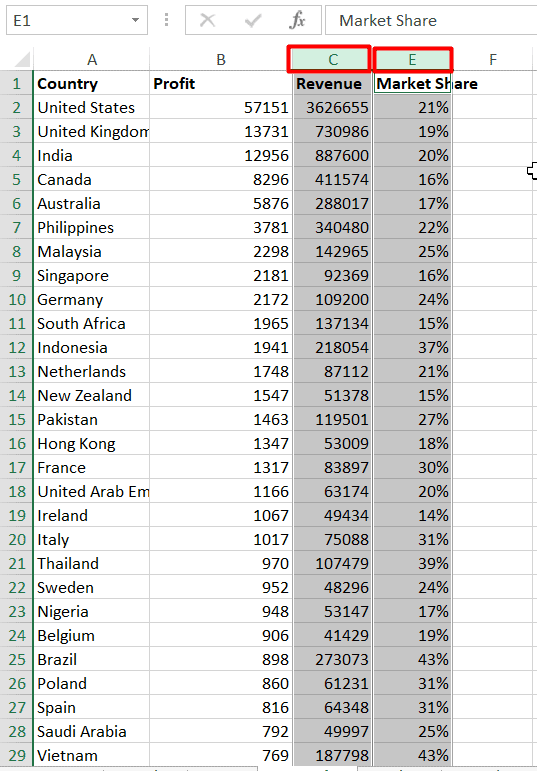
- Select the column data of what you need to hide – for instance, the column C.
- On a selected column to right-click of mouse and select the option «Hide» CTRL+0 (for columns) CTRL+9 (for rows).
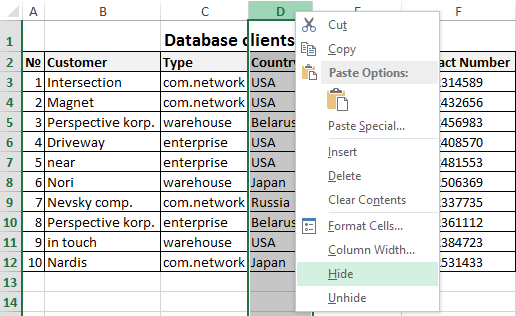
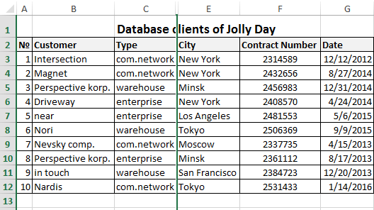
The column was hidden, but not deleted. This is evidenced by the priority of the alphabet`s letters in the names of columns (A; B; D; E).
Remark. If you want to hide multiple columns, highlight them before hiding. You can selectively highlight multiple columns with CTRL key pressed. In a similar way, you can hide the rows.
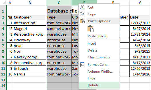
How to display hidden columns and rows in Excel?
To redisplay to the hidden column, you must select 2 of its contiguous (contiguous) columns. Then to generate the context menu, right-click and choose the option «Unhide».
The similar actions are performed in order to open the hidden rows in Excel.
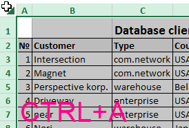
If the sheet is hidden many rows and columns and you want to display all at once, you must highlight the whole worksheet by pressing CTRL+A. Further a separate call to the context menu for the columns to choose the option «Show» and then for the rows, or in reverse order (for rows then for columns).
To select the entire sheet you can by clicking in the intersection of column headings and rows.
About these and other methods to select of an entire sheet and bands you have already known from the previous lessons.
Home > Microsoft Excel > How to Hide and Unhide Columns in Excel? (3 Easy Steps)
(Note: This guide on how to hide and unhide columns in Excel is suitable for all Excel versions including Office 365)
Excel comes with a whole package of features that helps us maintain and keep track of large sets of data. We have been covering these in our blogs.
In this guide, let us see one such important feature: How to hide and unhide columns in Excel?
But before we begin, let us understand why there is a need to hide or unhide columns in the first place. Hiding columns in Excel helps you organize your data better and makes it easier to understand for everyone. It does this by temporarily allowing you to hide certain columns, which you may consider irrelevant at present.
Now you may ask: Isn’t it better to delete them once and for all?
Yes, but in certain cases, you may need them later. Hence, it is advisable to hide them temporarily rather than delete them altogether. Let us quickly jump into the guide and learn how to do this the easy way.
You’ll learn:
- How to Hide Columns in Excel?
- How to Unhide Columns in Excel?
- How to Unhide All Hidden Columns in Excel?
Related:
How to Custom Sort Excel Data? 2 Easy Steps
How to Sort a Pivot Table in Excel? 6 Best Methods
How to Filter in Excel? A Step-by-Step Guide
How to Hide Columns in Excel?
Hiding columns in Excel is pretty straightforward. Just follow these steps:
- Open the Excel spreadsheet.
- Click on the Column name you want to hide. This will select the entire column.

- Let us say, you want to hide column ‘D’. Then, click on the letter ‘D’ in the columns section.
Pro Tip: If you want to select two or more columns at the same time, just keep clicking on the columns you want to hide while pressing the Ctrl key.
- Now that you have the relevant columns selected, all you have to do is just hide them. To do this, right-click inside any one of the selected columns and choose the ‘Hide’ option from the context menu.
That’s all. You have successfully hidden the selected columns. These hidden columns will be marked by a thicker green line in the spreadsheet.

Also Read:
How to Add Error Bars in Excel? 7 Best Methods
How to Enable Excel Dark Mode? 3 Simple Steps
How to Group Worksheets in Excel? (In 3 Simple Steps)
How to Unhide Columns in Excel?
Unhiding specific columns is also simple, provided you already know where these hidden columns lie.
First, let us see how to unhide a hidden column whose location we already know.
- Select the columns which engulf the hidden column by holding down the Shift key.
Let us say you want to unhide column ‘D’. Then you need to select both the columns ‘C’ and ‘A’ on both sides.
- Right-click on either selected column and choose ‘Unhide’ from the context menu.

- Alternatively, you can double click on or drag the hidden column marker to unhide it quickly.
How to Unhide All Hidden Columns in Excel?
Practically, it is impossible to keep track of all the hidden columns’ locations and unhide them one by one.
That’s why we need a one-stop solution to unhide all the hidden columns at the press of a button. Thankfully, Excel already has this feature labeled as the ‘Unhide Columns’ feature.
Follow these steps to use it:
- In the Home tab of the Excel ribbon menu, locate and click on the Format drop-down menu.
- In the drop-down list, click on the Hide & Unhide option in the Visibility section.
- This will once again open another list. Here, click on the Unhide Columns option.

This will unhide all the hidden columns in one go. This is a really helpful feature, especially if you have multiple hidden columns dispersed over a large spreadsheet. Alternatively, you can use the Ctrl+Shift+) shortcut.
Suggested Reads:
The Excel CHOOSE Function – 4 Best Uses
The FORMULATEXT Excel Function – 2 Best Examples
How to Make a Line Graph in Excel? 4 Best Line Graph Examples
FAQs
How to hide columns or rows in Excel using keyboard shortcuts?
To hide columns or rows in Excel using a keyboard shortcut, just select the relevant rows or columns and press the Ctrl+9 key combination. This will hide all selected columns and rows in one go. Note: The number ‘9’ from the numerical keypad may not work in some systems. Hence, it is advisable to use the normal number ‘9’ key.
How to hide all columns to the right of the last column in Excel?
In some cases, you may want to hide all empty columns on the right side of an Excel worksheet.
To do this, select the last column you want to use and press Ctrl+Shift+Right Arrow key combination, immediately followed by Ctrl+0. This will hide all unnecessary columns to the right of the main worksheet.
Let’s Wrap Up
In this short guide, we saw how to hide and unhide columns in Excel using traditional methods and shortcuts. The hide feature in Excel is one of the most rarely known but useful features out there. Using it wisely can save you and your teammates from a lot of confusion surrounding your worksheets. If you have any questions, please let us know in the comments.
If you need more high-quality Excel guides, please check out our free Excel resources center.
Simon Sez IT has been teaching Excel for over ten years. For a low, monthly fee you can get access to 130+ IT training courses. Click here for advanced Excel courses with in-depth training modules.
Simon Calder

Chris “Simon” Calder was working as a Project Manager in IT for one of Los Angeles’ most prestigious cultural institutions, LACMA.He taught himself to use Microsoft Project from a giant textbook and hated every moment of it. Online learning was in its infancy then, but he spotted an opportunity and made an online MS Project course — the rest, as they say, is history!
Содержание
- Алгоритмы скрытия
- Способ 1: сдвиг ячеек
- Способ 2: использование контекстного меню
- Способ 3: использование инструментов на ленте
- Вопросы и ответы

При работе с таблицами Excel иногда нужно скрыть определенные области листа. Довольно часто это делается в том случае, если в них, например, находятся формулы. Давайте узнаем, как можно спрятать столбцы в этой программе.
Алгоритмы скрытия
Существует несколько вариантов выполнить данную процедуру. Давайте выясним, в чем их суть.
Способ 1: сдвиг ячеек
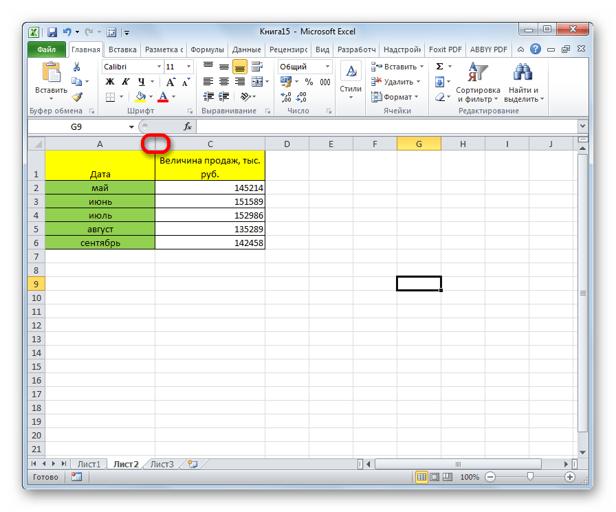
Наиболее интуитивно понятным вариантом, с помощью которого можно добиться нужного результата, является сдвиг ячеек. Для того, чтобы произвести данную процедуру, наводим курсор на горизонтальную панель координат в месте, где находится граница. Появляется характерная направленная в обе стороны стрелка. Кликаем левой кнопкой мыши и перетягиваем границы одного столбца к границам другого, насколько это можно сделать.
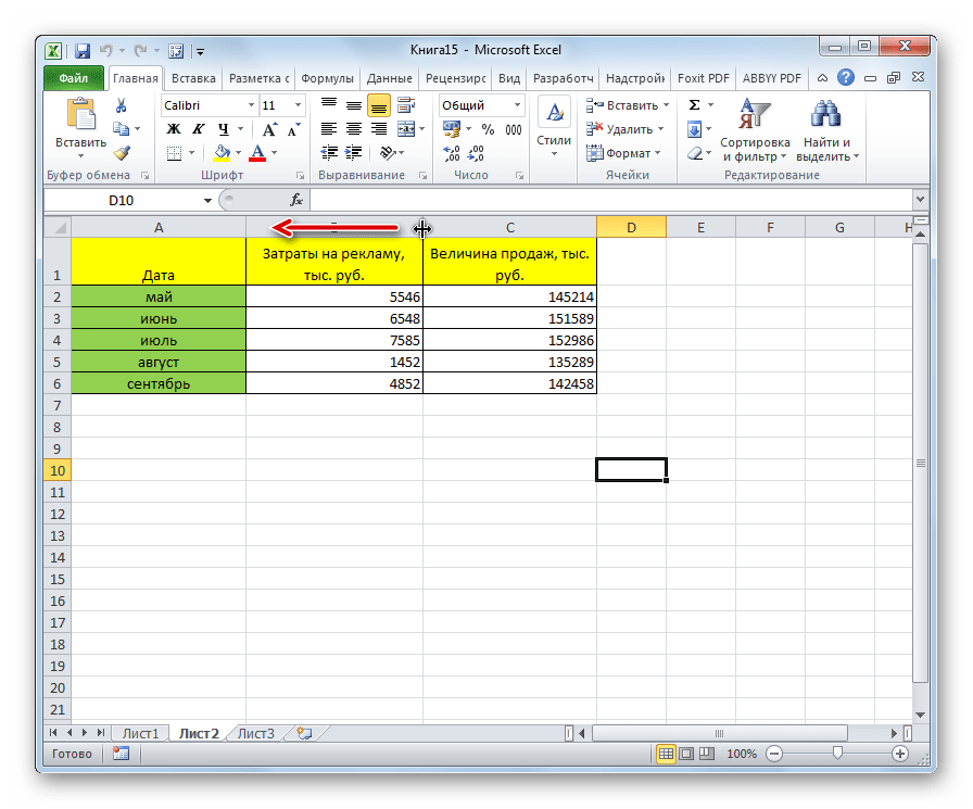
После этого, один элемент будет фактически скрыт за другим.
Способ 2: использование контекстного меню
Намного удобнее для данных целей использовать контекстное меню. Во-первых, это проще, чем двигать границы, во-вторых, таким образом, удаётся достигнуть полного скрытия ячеек, в отличие от предыдущего варианта.
- Кликаем правой кнопкой мыши по горизонтальной панели координат в области той латинской буквы, которой обозначен столбец подлежащий скрытию.
- В появившемся контекстном меню жмем на кнопку «Скрыть».
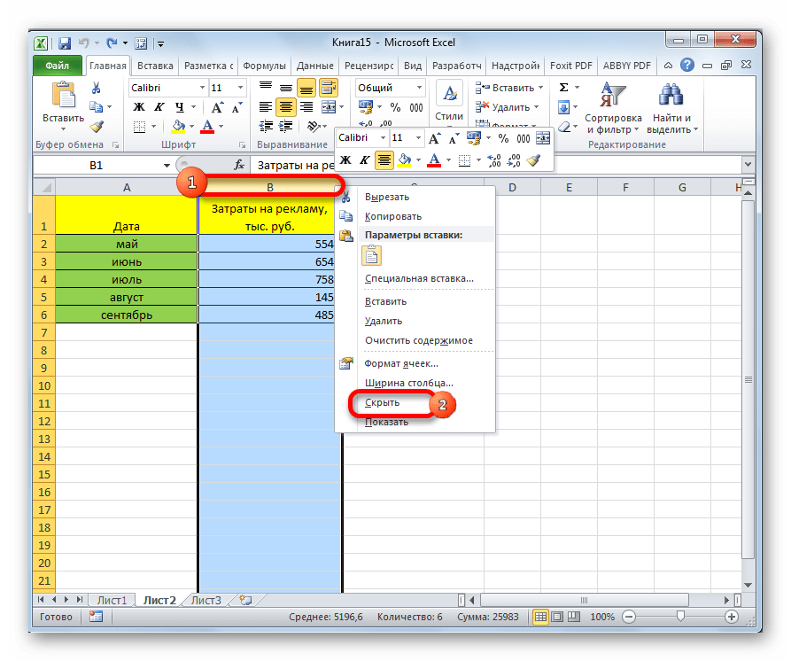
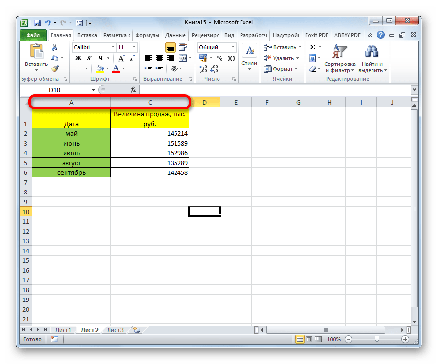
После этого, указанный столбец будет полностью скрыт. Для того, чтобы удостоверится в этом, взгляните на то, как обозначены столбцы. Как видим, в последовательном порядке не хватает одной буквы.
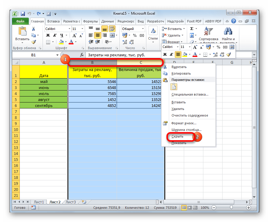
Преимущества данного способа перед предыдущим заключается и в том, что с помощью него можно прятать несколько последовательно расположенных столбцов одновременно. Для этого их нужно выделить, а в вызванном контекстном меню кликнуть по пункту «Скрыть». Если вы хотите произвести данную процедуру с элементами, которые не находятся рядом друг с другом, а разбросаны по листу, то выделение обязательно нужно проводить с зажатой кнопкой Ctrl на клавиатуре.
Способ 3: использование инструментов на ленте
Кроме того, выполнить эту процедуру можно при помощи одной из кнопок на ленте в блоке инструментов «Ячейки».
- Выделяем ячейки, расположенные в столбцах, которые нужно спрятать. Находясь во вкладке «Главная» кликаем по кнопке «Формат», которая размещена на ленте в блоке инструментов «Ячейки». В появившемся меню в группе настроек «Видимость» кликаем по пункту «Скрыть или отобразить». Активируется ещё один список, в котором нужно выбрать пункт «Скрыть столбцы».
- После этих действий, столбцы будут спрятаны.

Как и в предыдущем случае, таким образом можно прятать сразу несколько элементов, выделив их, как было описано выше.
Урок: Как отобразить скрытые столбцы в Excel
Как видим, существуют сразу несколько способов скрыть столбцы в программе Эксель. Наиболее интуитивным способом является сдвиг ячеек. Но, рекомендуется все-таки пользоваться одним из двух следующих вариантов (контекстное меню или кнопка на ленте), так как они гарантируют то, что ячейки будут полностью спрятаны. К тому же, скрытые таким образом элементы потом будет легче обратно отобразить при надобности.
Еще статьи по данной теме:
Помогла ли Вам статья?
Hide | Unhide | Multiple Columns or Rows | Hidden Tricks
Sometimes it can be useful to hide columns or rows in Excel.
Hide
To hide a column, execute the following steps.
1. Select a column.

2. Right click, and then click Hide.

Result:

Note: to hide a row, select a row, right click, and then click Hide.
Unhide
To unhide a column, execute the following steps.
1. Select the columns on either side of the hidden column.

2. Right click, and then click Unhide.

Result:

Note: to unhide a row, select the rows on either side of the hidden row, right click, and then click Unhide.
Multiple Columns or Rows
To hide multiple columns, execute the following steps.
1. Select multiple columns by clicking and dragging over the column headers.

2. To select non-adjacent columns, hold CTRL while clicking the column headers.

3. Right click, and then click Hide.
Result:

To unhide all columns, execute the following steps.
4. Select all columns by clicking the Select All button.

5. Right click a column header, and then click Unhide.
Result:

Note: in a similar way, you can hide and unhide multiple rows.
Hidden Tricks
Impress your boss with the following hidden  tricks. To hide and show columns with the click of a button, execute the following steps.
1. Select one or more columns.

2. On the Data tab, in the Outline group, click Group.

3. To hide the columns, click the minus sign.

4. To show the columns again, click the plus sign.

Note: to ungroup the columns, first, select the columns. Next, on the Data tab, in the Outline group, click Ungroup.
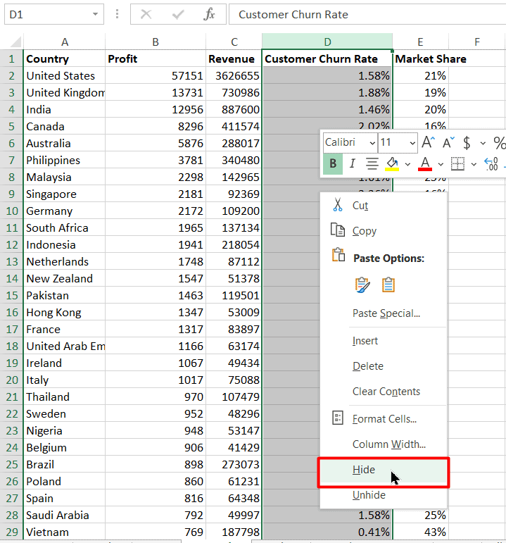
Finally, to hide cells in Excel, execute the following steps.
1. Select a range of cells.

2. Right click, and then click Format Cells.
The ‘Format Cells’ dialog box appears.
3. Select Custom.
4. Type the following number format code: ;;;
5. Click OK.

Result:

Note: the data is still there. Try it yourself. Download the Excel file, hide cells, select one of the hidden cells and look at the formula bar.
You have an Excel table with some unimportant rows, but you don’t want to delete them. In such case, you might want to “hide” them. There are two options of hiding rows (and columns): Either right-click on the row (or column) number and click on “Hide” or use the grouping function in order to create a group.
The Hide function (not recommended)
Many people love the “Hide” function for hiding rows or columns, because it is very easy to use: (the numbers are corresponding with the image)
- Mark the row(s) or column(s) that you want to hide.
- Right-click on the row number or column letter and click on “Hide”.
Unhide (all) hidden rows and columns
Unfortunately, hiding rows and columns has one big disadvantage: Hidden rows or columns are very hard to be seen. It’s only symbolized by a thin double line between the row or column number (3). A better way for hiding rows or columns is the Group function (4).
So, how to unhide all hidden rows?
Select the whole area in which you suspect hidden rows. Alternatively, select the whole worksheet in the top left corner. Now right-click on left-hand side with the row numbers (5) and click on “Unhide”.
Unhide all hidden rows and columns on all sheets at once
Do you want to show all hidden rows (and columns) on all the worksheets in your Excel file at the same time? It works almost the same way like for one worksheet except that you select all worksheets before.
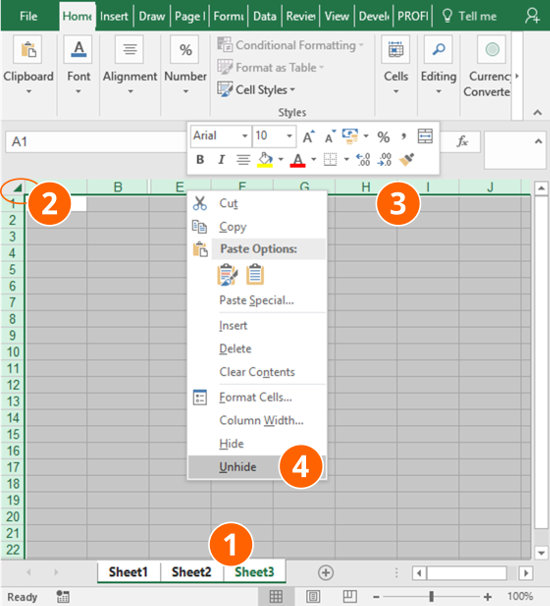
- Select all worksheets with hidden rows or columns.
- Select all columns, either by clicking on the top-left corner or by pressing Ctrl + A on the keyboard.
- Right-click on any column header (the letters A, B, C on top of each column) if you want to unhide columns. Right-click on any row number on the left-hand side if you want to unhide rows.
- Click on “Unhide”.
The Grouping function (recommended)
Grouping rows (or columns) has a big advantage: A little plus sign is shown, when you group rows. Because of that you can immediately see which rows are hidden. The hide function on the other hand only shows a “double” line which is not obvious and you could miss it easily.
Follow these steps for applying grouping:
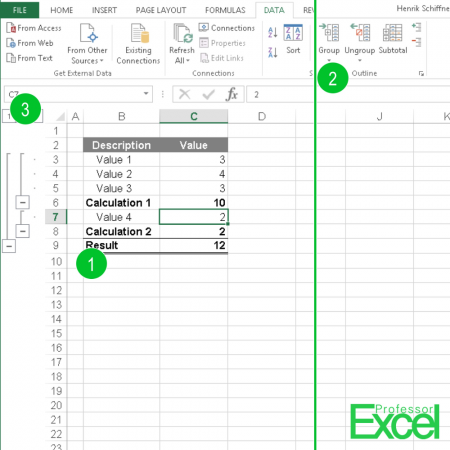
- Select the row or column you want to group.
- Click on “Group” on the Data ribbon. Alternatively, use the keyboard shortcut Alt + Shift + Arrow right for setting a Grouping or Alt + Shift + Arrow left for removing a Grouping
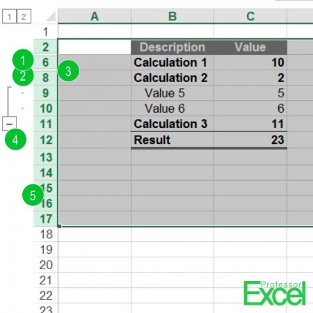
Grouping has one more feature: It allows you to set up Grouping levels. Let’s say, rows 3 to 5 and 7 are on level 2 and rows 6 and 8 (saying Calculation 1 and 2 in above picture) are level 2. If you press the small 1 in the top left corner, all groups on level 1 will be shown (see number 3 on the above picture).
Please note: If you run into some problems applying, opening, closing or removing grouping, please refer to these articles:
- Why I can’t add groupings to rows or columns in Excel?
- You can further define the direction of groupings: Do you want to set the grouping direction above or left of data in Excel?
Do you want to boost your productivity in Excel?
Get the Professor Excel ribbon!

Add more than 120 great features to Excel!
Expand or close all grouping on all worksheets simultaneously
In many cases you want to collapse all groupings or expand them. For example, before sending out a workbook, you might want to close all groups so that the workbook looks more “tidy” on the first impression. There are two methods for achieving this.
Method 1: Use a VBA macro for collapsing or expanding grouping
The following two VBA macros can either collapse all groupings or expand them.
Use these lines of code for collapsing everything to grouping level 1 (minimum).
Sub CollapsToMinimum()
    Dim ws As Worksheet
    For Each ws In Worksheets
        ws.Outline.ShowLevels RowLevels:=1, ColumnLevels:=1
    Next ws
End Sub
If you want to expand to show all groupings, expand the row and column levels to number 8 like in the following VBA code.
Sub ExpandToMaximum()
    Dim ws As Worksheet
    For Each ws In Worksheets
        ws.Outline.ShowLevels RowLevels:=8, ColumnLevels:=8
    Next ws
End Sub
Copy and paste this VBA code into a new module and press play. If you need assistance, please refer to this article.
Method 2: Use “Professor Excel Tools” for grouping, ungrouping, hiding and unhiding
If you got a large Excel file, you might want to expand or close all groups to the same level at the same time on more than on worksheet. Or expand them the maximum level or collapse them to the minimum level. For such task we created a function in our Excel add-in ‘Professor Excel Tools‘.
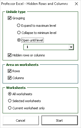
The function doesn’t only work on groupings, but also on hidden rows and columns:
- Define the grouping level: Minimum, maximum or the number of the level.
- Unhide all hidden rows or columns.
- Choose if you want to apply this action on rows, columns or both.
- Choose and which worksheets you want to use the hiding or unhiding action on: All worksheets, selected worksheets or the current worksheet only.
‘Professor Excel Tools’ is free to try. There are more than 120 other great functions included. You can download without any sign-up.

This function is included in our Excel Add-In ‘Professor Excel Tools’
(No sign-up, download starts directly)