

There may be times when you want to hide information in certain cells or hide entire rows or columns in an Excel worksheet. Maybe you have some extra data you reference in other cells that does not need to be visible.
We will show you how to hide cells and rows and columns in your worksheets and then show them again.
Update, 11/3/21: Looking to hide or unhide columns in Microsoft Excel? We have an updated guide for you.
RELATED: How to Hide or Unhide Columns in Microsoft Excel
Hide Cells
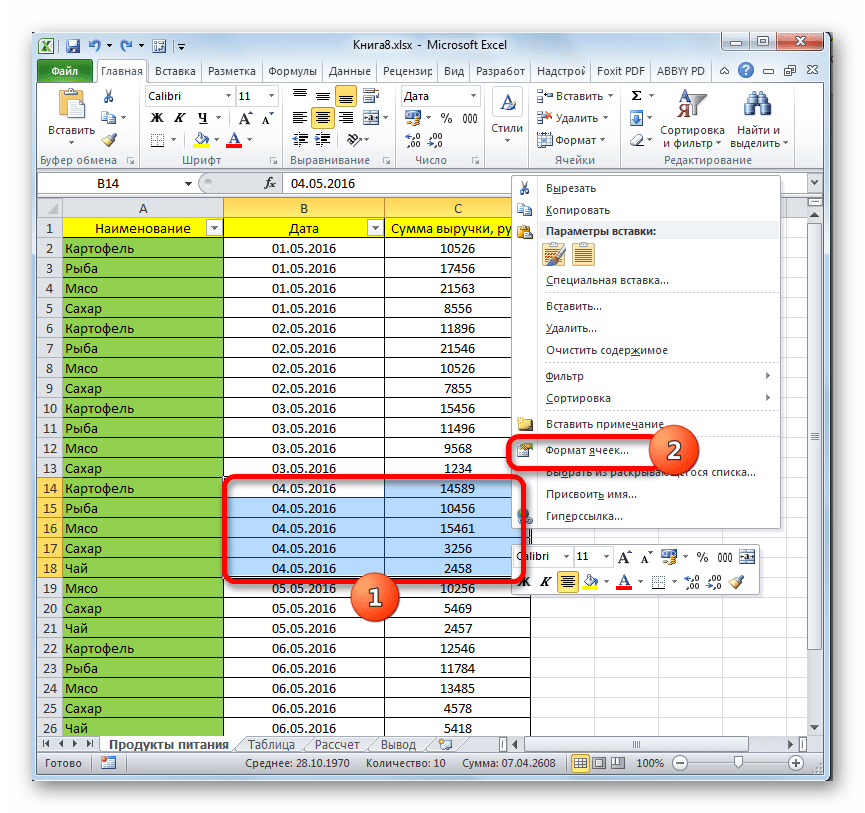
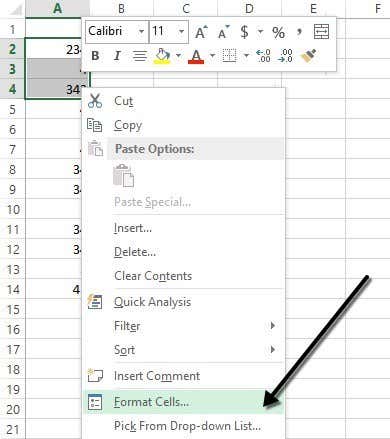
You can’t hide a cell in the sense that it completely disappears until you unhide it. With what would that cell be replaced? Excel can only blank out a cell so that nothing displays in the cell. Select individual cells or multiple cells using the “Shift” and “Ctrl” keys, just like you would when selecting multiple files in Windows Explorer. Right-click on any of the selected cells and select “Format Cells” from the popup menu.

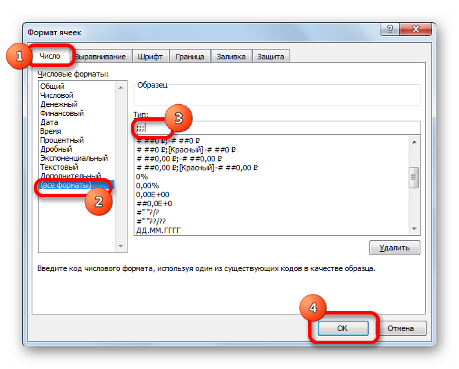
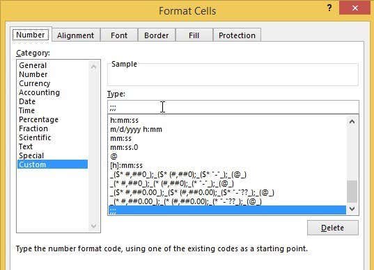
The “Format Cells” dialog box displays. Make sure the “Number” tab is active and select “Custom” in the “Category” list. In the “Type” edit box, enter three semicolons (;) without the parentheses and click “OK”.
NOTE: You might want to note what the “Type” was for each of the selected cells is before you change it so you can change the type of the cells back to what it was to show the content again.
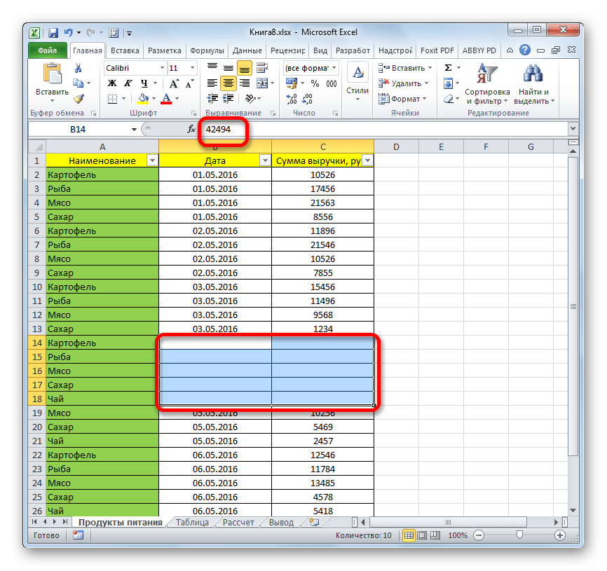
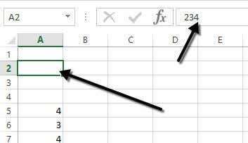
The data in the selected cells is now hidden, but the value or the formula is still in the cell and displays in the “Formula Bar”.
To unhide the content in the cells, follow the same steps listed above, but choose the original number category and type for the cells rather than “Custom” and the three semicolons.
NOTE: If you type anything into cells in which you hid the content, it will automatically be hidden after you press “Enter”. Also, the original value in the hidden cell will be replaced with the new value or formula that you type into the cell.
Hide Rows and Columns
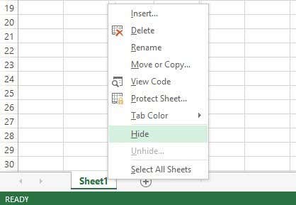
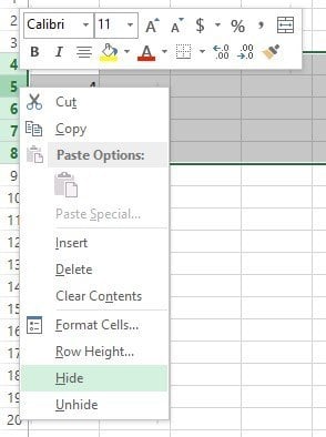
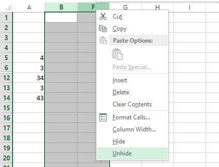
If you have a large worksheet, you might want to hide some rows and columns for data you don’t currently need to view. To hide an entire row, right-click on the row number and select “Hide”.
NOTE: To hide multiple rows, select the rows first by clicking and dragging over the range of rows you want to hide, and then right-click on the selected rows and select “Hide”. You can select non-sequential rows by pressing “Ctrl” as you click on the row numbers for the rows you want to select.
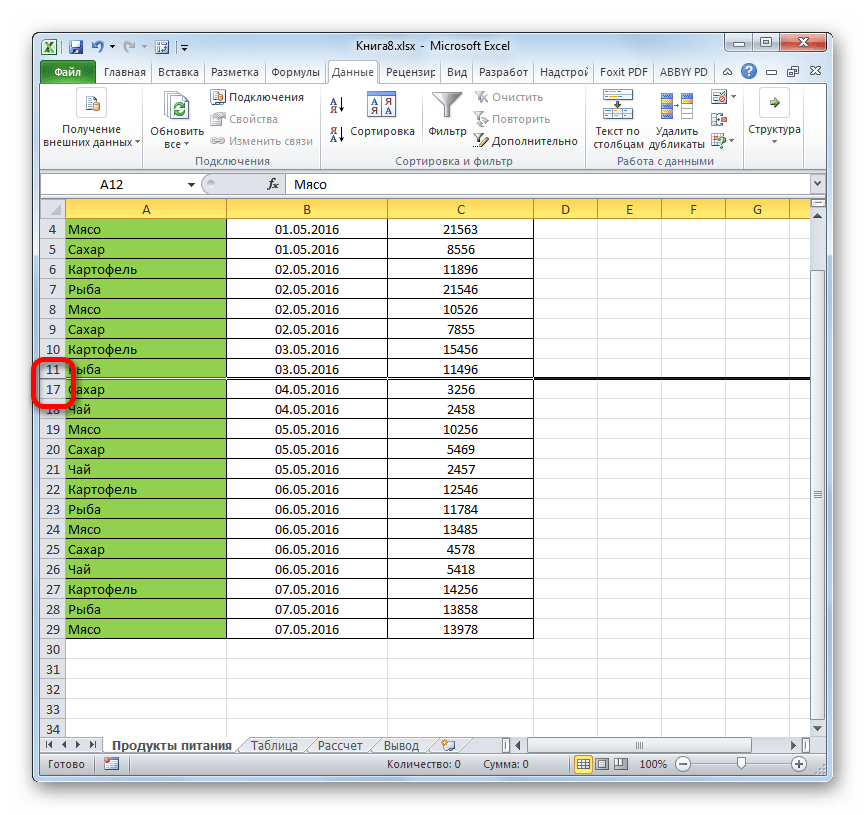
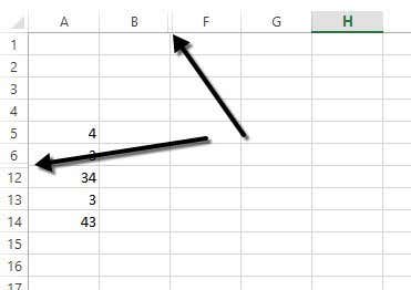
The hidden row numbers are skipped in the row number column and a double line displays in place of the hidden rows.
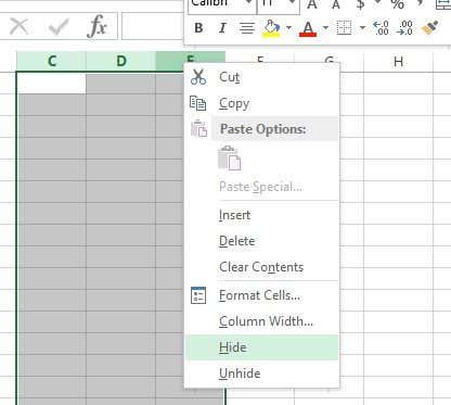
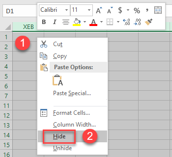
Hiding columns is a very similar process to hiding rows. Right-click on the column you want to hide, or select multiple column letters first and then right-click on the selected columns. Select “Hide” from the popup menu.
The hidden column letters are skipped in the row number column and a double line displays in place of the hidden rows.
To unhide a row or multiple rows, select the row before the hidden row(s) and the row after the hidden row(s) and right-click on the selection and select “Unhide” from the popup menu.
To unhide a column or multiple columns, select the two columns surrounding the hidden column(s), right-click on the selection, and select “Unhide” from the popup menu.
If you have a large spreadsheet and you don’t want to hide any cells, rows, or columns, you can freeze rows and columns so any headings you set up don’t scroll when you scroll through your data.
READ NEXT
- › How to Add and Remove Columns and Rows in Microsoft Excel
- › How to Copy and Paste Only Visible Cells in Microsoft Excel
- › How to Set Row Height and Column Width in Excel
- › How to Remove Blank Rows in Excel
- › How to Insert a Picture in Microsoft Excel
- › How to Use Custom Views in Excel to Save Your Workbook Settings
- › How to Count Checkboxes in Microsoft Excel
- › This New Google TV Streaming Device Costs Just $20
How-To Geek is where you turn when you want experts to explain technology. Since we launched in 2006, our articles have been read billions of times. Want to know more?
Содержание
- Процедура скрытия
- Способ 1: группировка
- Способ 2: перетягивание ячеек
- Способ 3: групповое скрытие ячеек перетягиванием
- Способ 4: контекстное меню
- Способ 5: лента инструментов
- Способ 6: фильтрация
- Способ 7: скрытие ячеек
- Вопросы и ответы

При работе в программе Excel довольно часто можно встретить ситуацию, когда значительная часть массива листа используется просто для вычисления и не несет информационной нагрузки для пользователя. Такие данные только занимают место и отвлекают внимание. К тому же, если пользователь случайно нарушит их структуру, то это может произвести к нарушению всего цикла вычислений в документе. Поэтому такие строки или отдельные ячейки лучше вообще скрыть. Кроме того, можно спрятать те данные, которые просто временно не нужны, чтобы они не мешали. Давайте узнаем, какими способами это можно сделать.
Процедура скрытия
Спрятать ячейки в Экселе можно несколькими совершенно разными способами. Остановимся подробно на каждом из них, чтобы пользователь сам смог понять, в какой ситуации ему будет удобнее использовать конкретный вариант.
Способ 1: группировка
Одним из самых популярных способов скрыть элементы является их группировка.
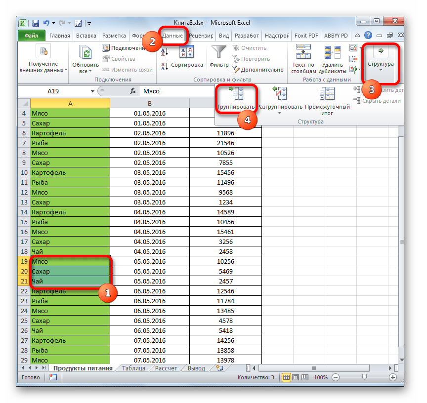
- Выделяем строки листа, которые нужно сгруппировать, а потом спрятать. При этом не обязательно выделять всю строку, а можно отметить только по одной ячейке в группируемых строчках. Далее переходим во вкладку «Данные». В блоке «Структура», который располагается на ленте инструментов, жмем на кнопку «Группировать».
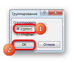
- Открывается небольшое окошко, которое предлагает выбрать, что конкретно нужно группировать: строки или столбцы. Так как нам нужно сгруппировать именно строки, то не производим никаких изменений настроек, потому что переключатель по умолчанию установлен в то положение, которое нам требуется. Жмем на кнопку «OK».
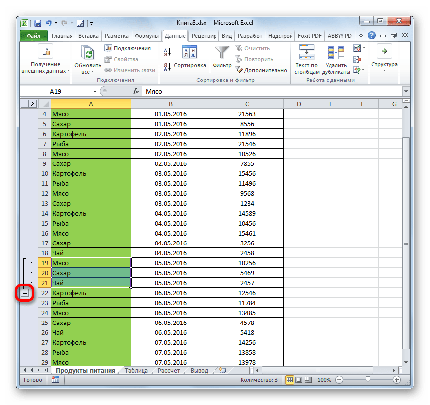
- После этого образуется группа. Чтобы скрыть данные, которые располагаются в ней, достаточно нажать на пиктограмму в виде знака «минус». Она размещается слева от вертикальной панели координат.
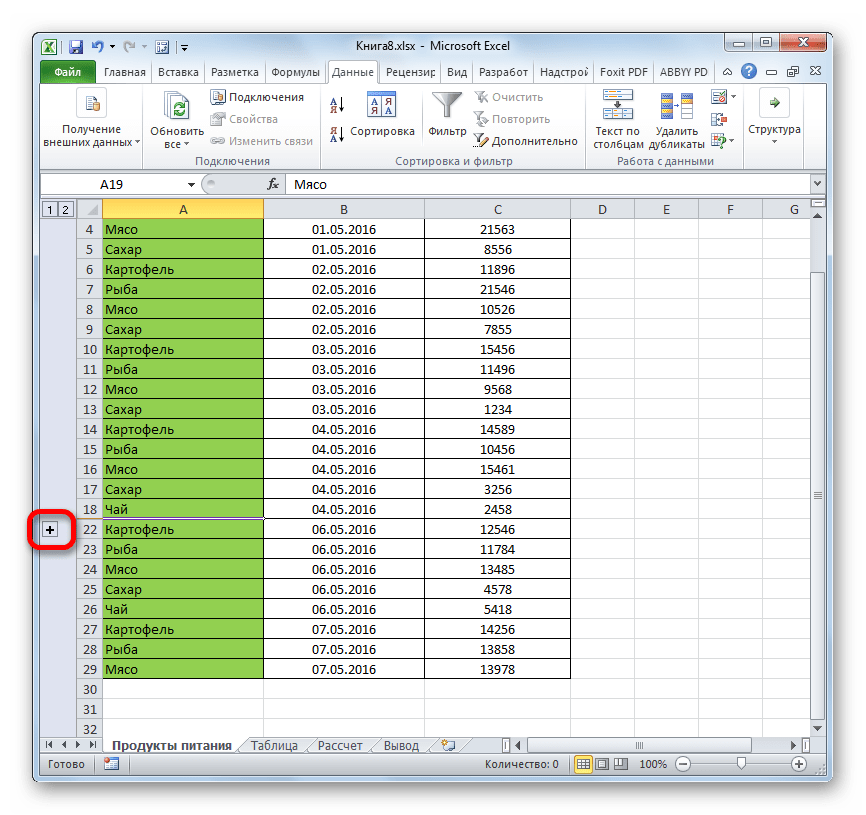
- Как видим, строки скрыты. Чтобы показать их снова, нужно нажать на знак «плюс».
Урок: Как сделать группировку в Excel
Способ 2: перетягивание ячеек
Самым интуитивно понятным способом скрыть содержимое ячеек, наверное, является перетягивание границ строк.
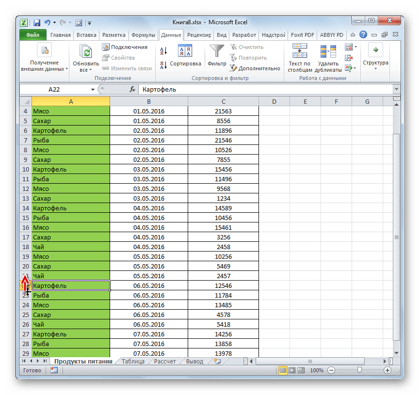
- Устанавливаем курсор на вертикальной панели координат, где отмечены номера строк, на нижнюю границу той строчки, содержимое которой хотим спрятать. При этом курсор должен преобразоваться в значок в виде креста с двойным указателем, который направлен вверх и вниз. Затем зажимаем левую кнопку мыши и тянем указатель вверх, пока нижняя и верхняя границы строки не сомкнутся.
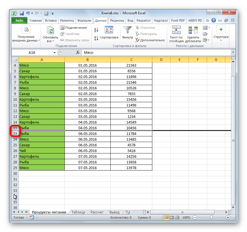
- Строка будет скрыта.
Способ 3: групповое скрытие ячеек перетягиванием
Если нужно таким методом скрыть сразу несколько элементов, то прежде их следует выделить.
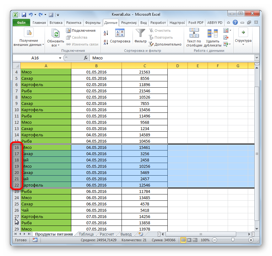
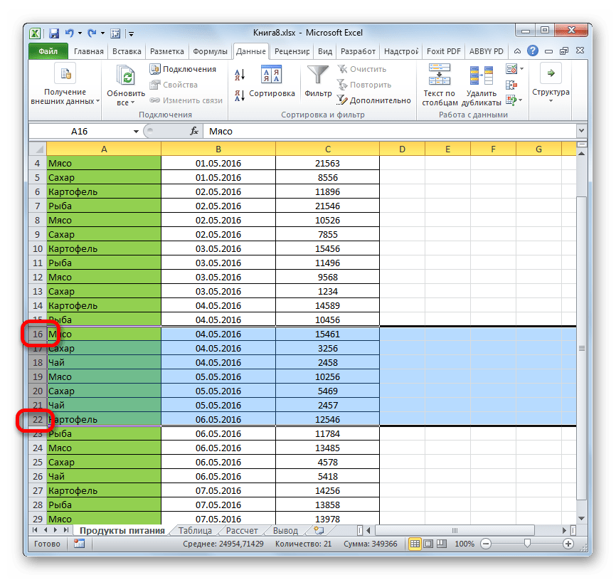
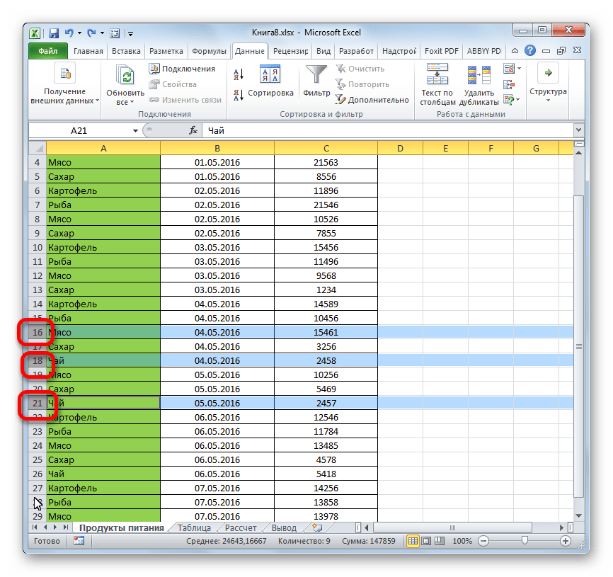
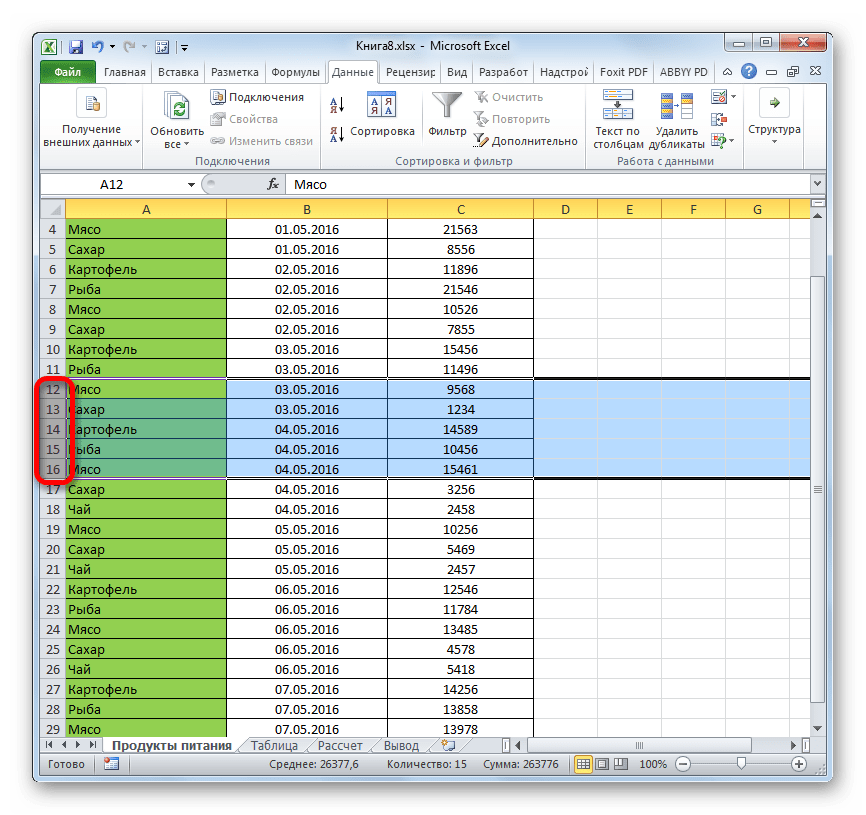
- Зажимаем левую кнопку мыши и выделяем на вертикальной панели координат группу тех строк, которые желаем скрыть.

Если диапазон большой, то выделить элементы можно следующим образом: кликаем левой кнопкой по номеру первой строчки массива на панели координат, затем зажимаем кнопку Shift и щелкаем по последнему номеру целевого диапазона.

Можно даже выделить несколько отдельных строк. Для этого по каждой из них нужно производить клик левой кнопкой мыши с зажатой клавишей Ctrl.
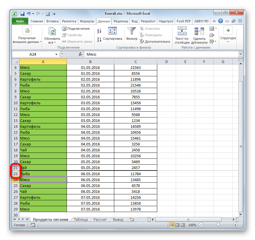
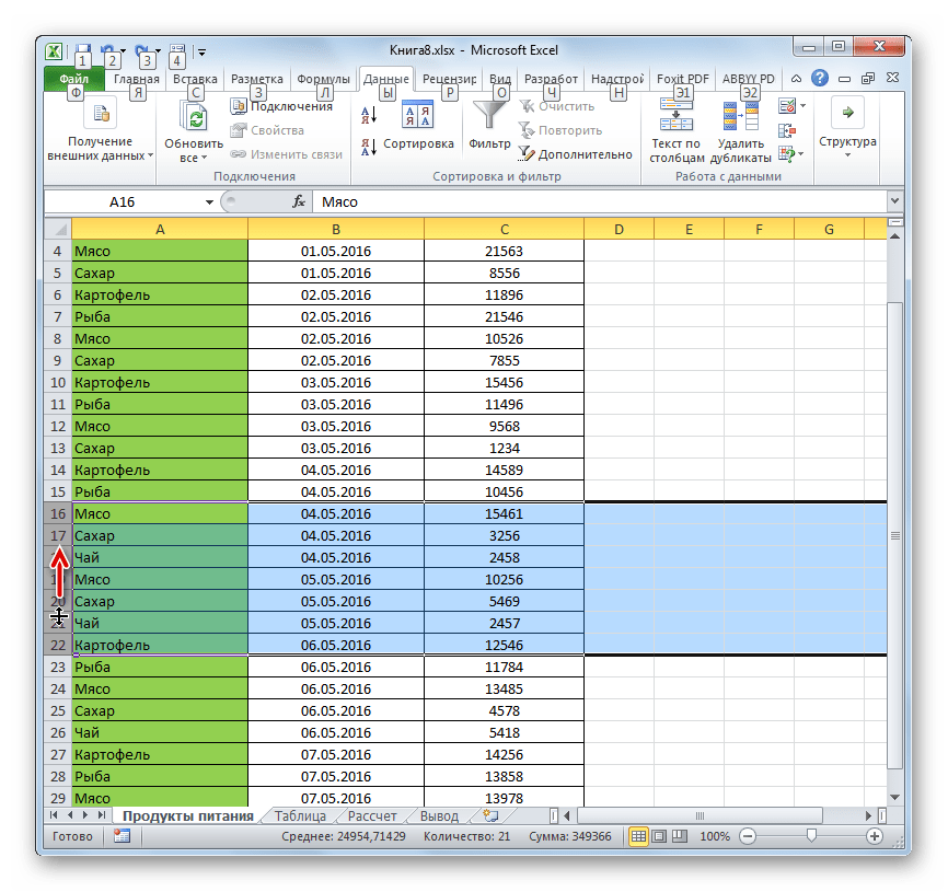
- Становимся курсором на нижнюю границу любой из этих строк и тянем её вверх, пока границы не сомкнутся.
- При этом будет скрыта не только та строка, над которой вы работаете, но и все строчки выделенного диапазона.

Способ 4: контекстное меню
Два предыдущих способа, конечно, наиболее интуитивно понятны и простые в применении, но они все-таки не могут обеспечить полного скрытия ячеек. Всегда остается небольшое пространство, зацепившись за которое можно обратно расширить ячейку. Полностью скрыть строку имеется возможность при помощи контекстного меню.
- Выделяем строчки одним из трёх способов, о которых шла речь выше:
- исключительно при помощи мышки;
- с использованием клавиши Shift;
- с использованием клавиши Ctrl.
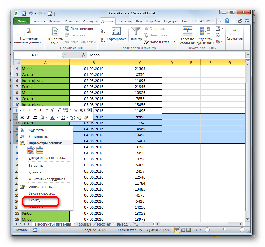
- Кликаем по вертикальной шкале координат правой кнопкой мыши. Появляется контекстное меню. Отмечаем пункт «Скрыть».
- Выделенные строки вследствие вышеуказанных действий будут скрыты.
Способ 5: лента инструментов
Также скрыть строки можно, воспользовавшись кнопкой на ленте инструментов.
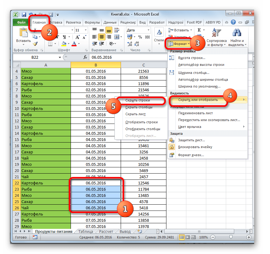
- Выделяем ячейки, находящиеся в строках, которые нужно скрыть. В отличие от предыдущего способа всю строчку выделять не обязательно. Переходим во вкладку «Главная». Щелкаем по кнопке на ленте инструментов «Формат», которая размещена в блоке «Ячейки». В запустившемся списке наводим курсор на единственный пункт группы «Видимость» — «Скрыть или отобразить». В дополнительном меню выбираем тот пункт, который нужен для выполнения поставленной цели – «Скрыть строки».
- После этого все строки, которые содержали выделенные в первом пункте ячейки, будут скрыты.
Способ 6: фильтрация
Для того, чтобы скрыть с листа содержимое, которое в ближайшее время не понадобится, чтобы оно не мешало, можно применить фильтрацию.
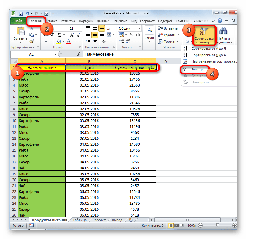
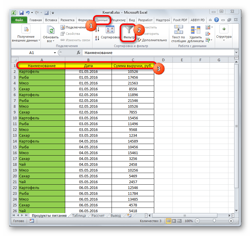
- Выделяем всю таблицу или одну из ячеек в её шапке. Во вкладке «Главная» жмем на значок «Сортировка и фильтр», который расположен в блоке инструментов «Редактирование». Открывается список действий, где выбираем пункт «Фильтр».

Можно также поступить иначе. После выделения таблицы или шапки переходим во вкладку «Данные». Кликам по кнопке «Фильтр». Она расположена на ленте в блоке «Сортировка и фильтр».
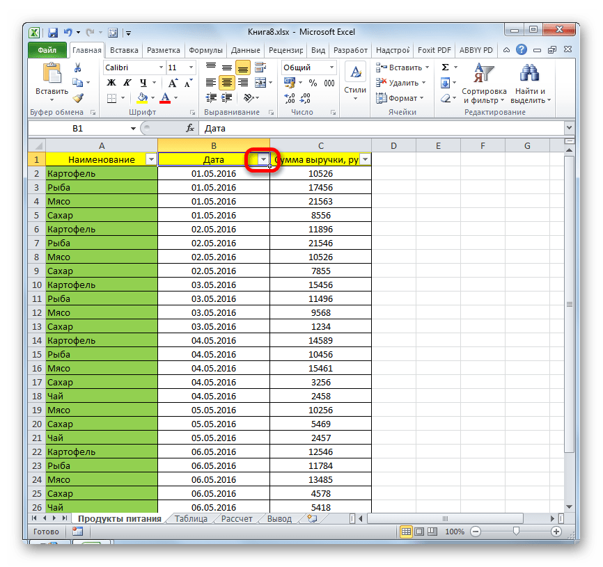
- Каким бы из двух предложенных способов вы не воспользовались, в ячейках шапки таблицы появится значок фильтрации. Он представляет собой небольшой треугольник черного цвета, направленный углом вниз. Кликаем по этому значку в той колонке, где содержится признак, по которому мы будем фильтровать данные.
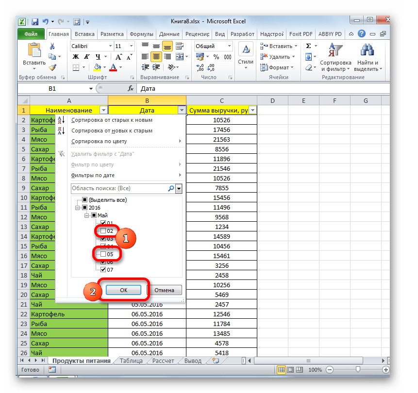
- Открывается меню фильтрации. Снимаем галочки с тех значений, которые содержатся в строках, предназначенных для скрытия. Затем жмем на кнопку «OK».
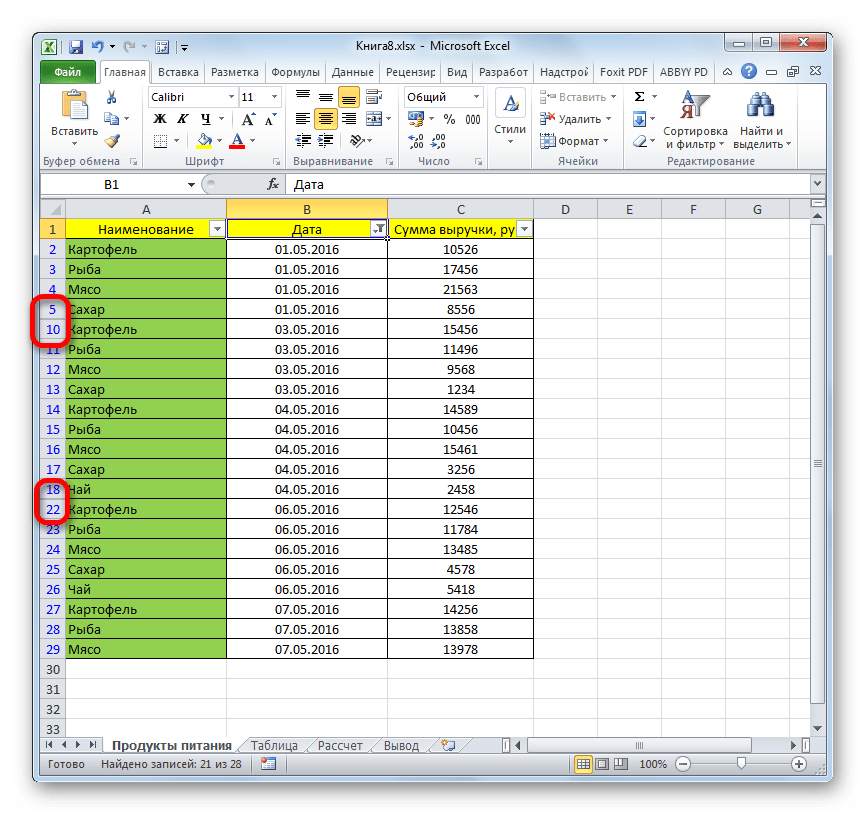
- После этого действия все строки, где имеются значения, с которых мы сняли галочки, будут скрыты при помощи фильтра.
Урок: Сортировка и фильтрация данных в Excel
Способ 7: скрытие ячеек
Теперь поговорим о том, как скрыть отдельные ячейки. Естественно их нельзя полностью убрать, как строчки или колонки, так как это разрушит структуру документа, но все-таки существует способ, если не полностью скрыть сами элементы, то спрятать их содержимое.
- Выделяем одну или несколько ячеек, которые нужно спрятать. Кликаем по выделенному фрагменту правой кнопкой мыши. Открывается контекстное меню. Выбираем в нем пункт «Формат ячейки…».
- Происходит запуск окна форматирования. Нам нужно перейти в его вкладку «Число». Далее в блоке параметров «Числовые форматы» выделяем позицию «Все форматы». В правой части окна в поле «Тип» вбиваем следующее выражение:
;;;Жмем на кнопку «OK» для сохранения введенных настроек.
- Как видим, после этого все данные в выделенных ячейках исчезли. Но они исчезли только для глаз, а по факту продолжают там находиться. Чтобы удостоверится в этом, достаточно взглянуть на строку формул, в которой они отображаются. Если снова понадобится включить отображение данных в ячейках, то нужно будет через окно форматирования поменять в них формат на тот, что был ранее.
Как видим, существует несколько разных способов, с помощью которых можно спрятать строки в Экселе. Причем большинство из них используют совершенно разные технологии: фильтрация, группировка, сдвиг границ ячеек. Поэтому пользователь имеет очень широкий выбор инструментов для решения поставленной задачи. Он может применить тот вариант, который считает более уместным в конкретной ситуации, а также более удобным и простым для себя. Кроме того, с помощью форматирования имеется возможность скрыть содержимое отдельных ячеек.
Еще статьи по данной теме:
Помогла ли Вам статья?
If you use Excel on a daily basis, then you’ve probably run into situations where you needed to hide something in your Excel worksheet. Maybe you have some extra data worksheets that are referenced, but don’t need to be viewed. Or maybe you have a few rows of data at the bottom of the worksheet that need to be hidden.
There are a lot of different parts to an Excel spreadsheet and each part can be hidden in different ways. In this article, I’ll walk you through the different content that can be hidden in Excel and how to get view the hidden data at a later time.
How to Hide Tabs/WorkSheets
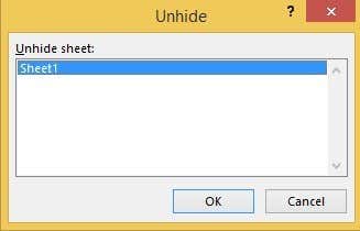
In order to hide a worksheet or tab in Excel, right-click on the tab and choose Hide. That was pretty straightforward.
Once hidden, you can right-click on a visible sheet and select Unhide. All hidden sheets will be shown in a list and you can select the one you want to unhide.
Excel does not have the ability to hide a cell in the traditional sense that they simply disappear until you unhide them, like in the example above with sheets. It can only blank out a cell so that it appears that nothing is in the cell, but it can’t truly “hide” a cell because if a cell is hidden, what would you replace that cell with?
You can hide entire rows and columns in Excel, which I explain below, but you can only blank out individual cells. Right-click on a cell or multiple selected cells and then click on Format Cells.
On the Number tab, choose Custom at the bottom and enter three semicolons (;;;) without the parentheses into the Type box.
Click OK and now the data in those cells is hidden. You can click on the cell and you should see the cell remains blank, but the data in the cell shows up in the formula bar.
To unhide the cells, follow the same procedure above, but this time choose the original format of the cells rather than Custom. Note that if you type anything into those cells, it will automatically be hidden after you press Enter. Also, whatever original value was in the hidden cell will be replaced when typing into the hidden cell.
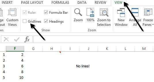
Hide Gridlines
A common task in Excel is hiding gridlines to make the presentation of the data cleaner. When hiding gridlines, you can either hide all gridlines on the entire worksheet or you can hide gridlines for a certain portion of the worksheet. I will explain both options below.
To hide all gridlines, you can click on the View tab and then uncheck the Gridlines box.
You can also click on the Page Layout tab and uncheck the View box under Gridlines.

How to Hide Rows and Columns
If you want to hide an entire row or column, right-click on the row or column header and then choose Hide. To hide a row or multiple rows, you need to right-click on the row number at the far left. To hide a column or multiple columns, you need to right-click on the column letter at the very top.
You can easily tell there are hidden rows and columns in Excel because the numbers or letters skip and there are two visible lines shown to indicate hidden columns or rows.
To unhide a row or column, you need to select the row/column before and the row/column after the hidden row/column. For example, if Column B is hidden, you would need to select column A and column C and then right-click and choose Unhide to unhide it.
How to Hide Formulas
Hiding formulas is slightly more complicated than hiding rows, columns, and tabs. If you want to hide a formula, you have to do TWO things: set the cells to Hidden and then protect the sheet.
So, for example, I have a sheet with some proprietary formulas that I don’t want anyone to see!

First, I will select the cells in column F, right-click and choose Format Cells. Now click on the Protection tab and check the box that says Hidden.
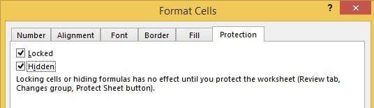
As you can see from the message, hiding formulas won’t go into effect until you actually protect the worksheet. You can do this by clicking on the Review tab and then clicking on Protect Sheet.
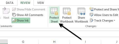
You can enter in a password if you want to prevent people from un-hiding the formulas. Now you’ll notice that if you try to view the formulas, by pressing CTRL + ~ or by clicking on Show Formulas on the Formulas tab, they will not be visible, however, the results of that formula will remain visible.
Hide Comments
By default, when you add a comment to an Excel cell, it will show you a small red arrow in the upper right corner to indicate there is a comment there. When you hover over the cell or select it, the comment will appear in a pop up window automatically.
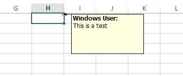
You can change this behavior so that the arrow and the comment are not shown when hovering or selecting the cell. The comment will still remain and can be viewed by simply going to the Review tab and clicking on Show All Comments. To hide the comments, click on File and then Options.
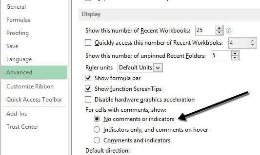
Click on Advanced and then scroll down to the Display section. There you will see an option called No comment or indicators under the For cells with comments, show: heading.
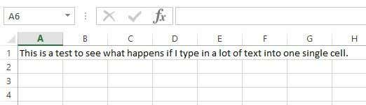
Hide Overflow Text
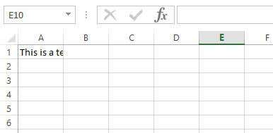
In Excel, if you type a lot of text into a cell, it will simply overflow over the adjacent cells. In the example below, the text only exists in cell A1, but it overflows to other cells so that you can see it all.
If I were to type something into cell B1, it would then cut off the overflow and show the contents of B1. If you want this behavior without having to type anything into the adjacent cell, you can right-click on the cell, choose Format Cells and then select Fill from the Horizontal Text alignment drop down box.
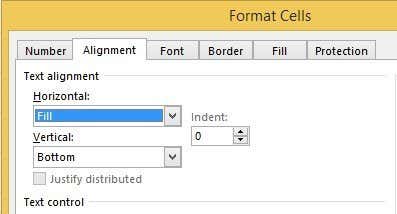
This will hide the overflow text for that cell even if nothing is in the adjacent cell. Note that this is kind of a hack, but it works most of the time.
You could also choose Format Cells and then check the Wrap Text box under Text control on the Alignment tab, but that will increase the height of the row. To get around that, you could simply right-click on the row number and then click on Row Height to adjust the height back to its original value. Either of these two methods will work for hiding overflow text.
Hide Workbook
I’m not sure why you would want or need to do this, but you can also click on the View tab and click on the Hide button under Split. This will hide the entire workbook in Excel! There is absolutely nothing you can do other than clicking on the Unhide button to bring back the workbook.
So now you’ve learnt how to hide workbooks, sheets, rows, columns, gridlines, comments, cells, and formulas in Excel! If you have any questions, post a comment. Enjoy!
Hide or show rows or columns
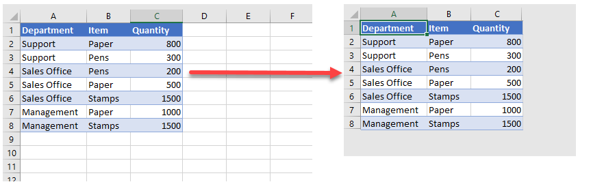
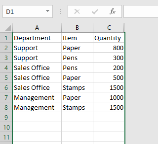
Hide or unhide columns in your spreadsheet to show just the data that you need to see or print.

Hide columns
-
Select one or more columns, and then press Ctrl to select additional columns that aren’t adjacent.
-
Right-click the selected columns, and then select Hide.
Note: The double line between two columns is an indicator that you’ve hidden a column.
Unhide columns
-
Select the adjacent columns for the hidden columns.
-
Right-click the selected columns, and then select Unhide.
Or double-click the double line between the two columns where hidden columns exist.
Need more help?
You can always ask an expert in the Excel Tech Community or get support in the Answers community.
See Also
Unhide the first column or row in a worksheet
Need more help?
See all How-To Articles
This tutorial demonstrates how to hide cells in Excel and Google Sheets.
Hide Unused Cells – Excel Ribbon
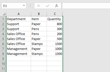
Hide Unused Columns
Excel doesn’t give you the option to hide individual cells, but you can hide unused rows and columns in order to display only the working area. To hide unused columns using the Ribbon, follow these steps:
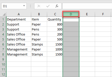
- First, select the column header in the first empty column and press CTRL + SHIFT + → to select all the columns between the selected one and the last one.
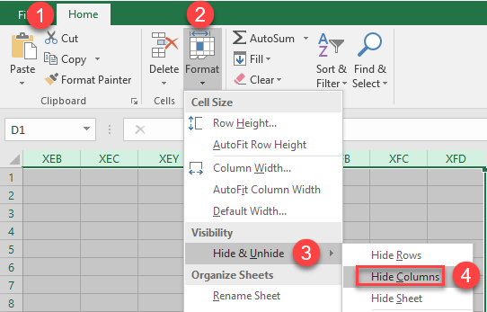
- Then, in the Ribbon, go to Home > Format > Hide & Unhide > Hide Columns.
As a result, all selected columns are hidden.
Hide Unused Rows
To hide all unused rows using the Ribbon, follow these steps:
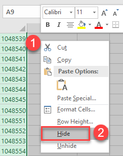
- Select the row header for the first empty row and then press CTRL + SHIFT + ↓ to select all the rows between the selected one and the last one.
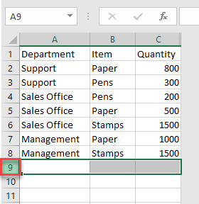
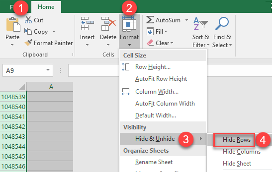
- In the Ribbon go to Home > Format > Hide & Unhide > Hide Rows.
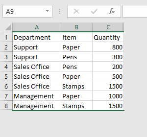
Now, all unused rows are hidden, and only populated cells are shown.
Hide Unused Cells – Context Menu
Hide Unused Columns
Another way to hide unused columns in Excel is by using the context menu.
- Select the column header in the first empty column and press CTRL + SHIFT + → to select all columns between the selected one and the last one.
- Right-click anywhere in the sheet and from the context menu, choose Hide.
All selected columns are hidden after this step.
Hide Unused Rows
To hide all unused rows using the context menu in Excel:
- Select the row header in the first empty row and then press CTRL + SHIFT + ↓ to select all the rows between the selected one and the last one.
- After that step, right-click anywhere in the sheet and from the context menu, choose Hide.
As a result, all unused rows are hidden, and only populated cells are displayed.
Hide Unused Cells in Google Sheets
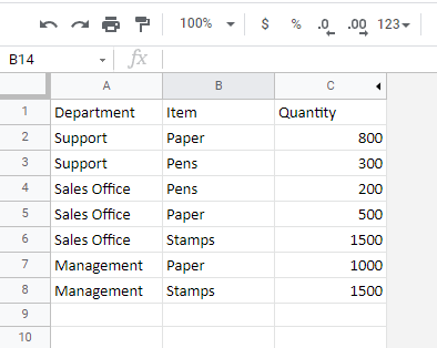
To hide unused cells in Google Sheets and display only the working area, you also need to hide rows and columns.
Hide Columns
- Select the column header in the first empty column and press CTRL + SHIFT + → to select all the columns between the selected one and the last one.
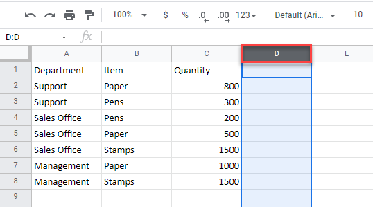
- After that, right-click anywhere on the selected range and choose Hide columns (here, Hide columns D – Z).
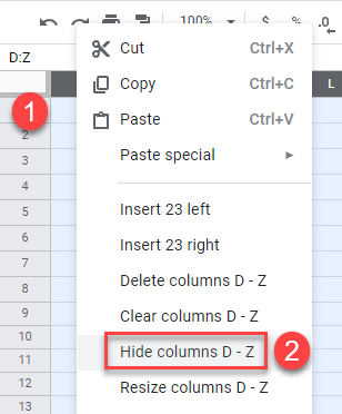
This hides all selected columns.
Hide Rows
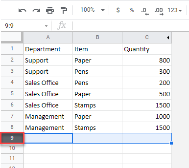
- To hide all unused rows in Google Sheets, select the row header in the first empty row and press CTRL + SHIFT + ↓ to select all the rows between the selected one and the last one.
- Then, right-click anywhere on the selected area and from the Menu, choose Hide rows (here, Hide rows 9 – 1000).
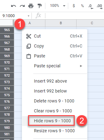
As a result, all selected rows are hidden, and only populated cells are shown.
See also…
- How to Hide and Unhide Workbooks
- How to Hide and Unhide Worksheets
- How to Hide Column and Row Headings
- How to Hide Vertical and Horizontal Scroll Bars
- How to Show and Hide Gridlines
- How to Delete Infinite Rows and Columns
Learn several ways to do this
Updated on September 19, 2022
What to Know
- Hide a column: Select a cell in the column to hide, then press Ctrl+0. To unhide, select an adjacent column and press Ctrl+Shift+0.
- Hide a row: Select a cell in the row you want to hide, then press Ctrl+9. To unhide, select an adjacent column and press Ctrl+Shift+9.
- You can also use the right-click context menu and the format options on the Home tab to hide or unhide individual rows and columns.
You can hide columns and rows in Excel to make a cleaner worksheet without deleting data you might need later, although there is no way to hide individual cells. In this guide, we provide instructions for three ways to hide and unhide columns in Excel 2019, 2016, 2013, 2010, 2007, and Excel for Microsoft 365.
Hide Columns in Excel Using a Keyboard Shortcut
The keyboard key combination for hiding columns is Ctrl+0.
-
Click on a cell in the column you want to hide to make it the active cell.
-
Press and hold down the Ctrl key on the keyboard.
-
Press and release the 0 key without releasing the Ctrl key. The column containing the active cell should be hidden from view.
To hide multiple columns using the keyboard shortcut, highlight at least one cell in each column to be hidden, and then repeat steps two and three above.
Hide Columns Using the Context Menu
The options available in the context — or right-click menu — change depending upon the object selected when you open the menu. If the Hide option, as shown in the image below, is not available in the context menu it is likely that you didn’t select the entire column before right-clicking.
Hide a Single Column
-
Click the column header of the column you want to hide to select the entire column.
-
Right-click on the selected column to open the context menu.
-
Choose Hide. The selected column, the column letter, and any data in the column will be hidden from view.
Hide Adjacent Columns
-
In the column header, click and drag with the mouse pointer to highlight all three columns.
-
Right-click on the selected columns.
-
Choose Hide. The selected columns and column letters will be hidden from view.
When you hide columns and rows containing data, it does not delete the data, and you can still reference it in formulas and charts. Hidden formulas containing cell references will update if the data in the referenced cells changes.
Hide Separated Columns
-
In the column header click on the first column to be hidden.
-
Press and hold down the Ctrl key on the keyboard.
-
Continue to hold down the Ctrl key and click once on each additional column to be hidden to select them.
-
Release the Ctrl key.
-
In the column header, right-click on one of the selected columns and choose Hide. The selected columns and column letters will be hidden from view.
When hiding separate columns, if the mouse pointer is not over the column header when you click the right mouse button, the hide option will not be available.
Hide and Unhide Columns in Excel Using the Name Box
This method can be used to unhide any single column. In our example, we will be using column A.
-
Type the cell reference A1 into the Name Box.
-
Press the Enter key on the keyboard to select the hidden column.
-
Click on the Home tab of the ribbon.
-
Click on the Format icon on the ribbon to open the drop-down.
-
In the Visibility section of the menu, choose Hide & Unhide > Hide Columns or Unhide Column.
Unhide Columns Using a Keyboard Shortcut
The key combination for unhiding columns is Ctrl+Shift+0.
-
Type the cell reference A1 into the Name Box.
-
Press the Enter key on the keyboard to select the hidden column.
-
Press and hold down the Ctrl and the Shift keys on the keyboard.
-
Press and release the 0 key without releasing the Ctrl and Shift keys.
To unhide one or more columns, highlight at least one cell in the columns on either side of the hidden column(s) with the mouse pointer.
-
Click and drag with the mouse to highlight columns A to G.
-
Press and hold down the Ctrl and the Shift keys on the keyboard.
-
Press and release the 0 key without releasing the Ctrl and Shift keys. The hidden column(s) will become visible.
The Ctrl+Shift+0 keyboard shortcut might not work depending on the version of Windows you’re running, for reasons not explained by Microsoft. If this shortcut doesn’t work, use another method from the article.
Unhide Columns Using the Context Menu
As with the shortcut key method above, you must select at least one column on either side of a hidden column or columns to unhide them. For example, to unhide columns D, E, and G:
-
Hover the mouse pointer over column C in the column header. Click and drag with the mouse to highlight columns C to H to unhide all columns at one time.
-
Right-click on the selected columns and choose Unhide. The hidden column(s) will become visible.
Hide Rows Using Shortcut Keys
The keyboard key combination for hiding rows is Ctrl+9:
-
Click on a cell in the row you want to hide to make it the active cell.
-
Press and hold down the Ctrl key on the keyboard.
-
Press and release the 9 key without releasing the Ctrl key. The row containing the active cell should be hidden from view.
To hide multiple rows using the keyboard shortcut, highlight at least one cell in each row you want to hide, and then repeat steps two and three above.
Hide Rows Using the Context Menu
The options available in the context menu — or right-click — change depending upon the object selected when you open it. If the Hide option, as shown in the image above, is not available in the context menu it is because you probably didn’t select the entire row.
Hide a Single Row
-
Click on the row header for the row to be hidden to select the entire row.
-
Right-click on the selected row to open the context menu.
-
Choose Hide. The selected row, the row letter, and any data in the row will be hidden from view.
Hide Adjacent Rows
-
In the row header, click and drag with the mouse pointer to highlight all three rows.
-
Right-click on the selected rows and choose Hide. The selected rows will be hidden from view.
Hide Separated Rows
-
In the row header, click on the first row to be hidden.
-
Press and hold down the Ctrl key on the keyboard.
-
Continue to hold down the Ctrl key and click once on each additional row to be hidden to select them.
-
Right-click on one of the selected rows and choose Hide. The selected rows will be hidden from view.
Hide and Unhide Rows Using the Name Box
This method can be used to unhide any single row. In our example, we will be using row 1.
-
Type the cell reference A1 into the Name Box.
-
Press the Enter key on the keyboard to select the hidden row.
-
Click on the Home tab of the ribbon.
-
Click on the Format icon on the ribbon to open the drop-down menu.
-
In the Visibility section of the menu, choose Hide & Unhide > Hide Rows or Unhide Row.
Unhide Rows Using a Keyboard Shortcut
The key combination for unhiding rows is Ctrl+Shift+9.
Unhide Rows using Shortcut Keys and Name Box
-
Type the cell reference A1 into the Name Box.
-
Press the Enter key on the keyboard to select the hidden row.
-
Press and hold down the Ctrl and the Shift keys on the keyboard.
-
Press and hold down the Ctrl and the Shift keys on the keyboard. Row 1 will become visible.
Unhide Rows Using a Keyboard Shortcut
To unhide one or more rows, highlight at least one cell in the rows on either side of the hidden row(s) with the mouse pointer. For example, you want to unhide rows 2, 4, and 6.
-
To unhide all rows, click and drag with the mouse to highlight rows 1 to 7.
-
Press and hold down the Ctrl and the Shift keys on the keyboard.
-
Press and release the number 9 key without releasing the Ctrl and Shift keys. The hidden row(s) will become visible.
Unhide Rows Using the Context Menu
As with the shortcut key method above, you must select at least one row on either side of a hidden row or rows to unhide them. For example, to unhide rows 3, 4, and 6:
-
Hover the mouse pointer over row 2 in the row header.
-
Click and drag with the mouse to highlight rows 2 to 7 to unhide all rows at one time.
-
Right-click on the selected rows and choose Unhide. The hidden row(s) will become visible.
How to Move Columns in Excel
FAQ
-
How do I hide cells in Excel?
Select the cell or cells you want to hide, then select the Home tab > Cells > Format > Format Cells. In the Format Cells menu, select the Number tab > Custom (under Category) and type ;;; (three semicolons), then select OK.
-
How do I hide gridlines in Excel?
Select the Page Layout tab, then turn off the View checkbox under Gridlines.
-
How do I hide formulas in Excel?
Select the cells with formulas you want to hide > select the Hidden checkbox on the Protection tab > OK > Review > Protect Sheet. Next, verify that Protect worksheet and contents of locked cells is turned on, then select OK.
Thanks for letting us know!
Get the Latest Tech News Delivered Every Day
Subscribe
Making things invisible in Excel
March 20 2015 Written By: EduPristine
As kids everybody loved going to the magic show and see the things disappearing like the hats, sticks and sometimes people. Well, we can’t help you in making people disappear but we would definitely love to show you some tricks that will help you to hide certain things in Excel.
Hiding cells
Steps to hide cells in Excel
1. Select the cells that needs to be hidden. In our example it is B2:B5
2. Right click and open the format cell dailog box or you can use the shortcut key Ctrl + 1

3. On the number tab, select the custom option that is available at extreme bottom.
4. Type the formatting code as “;;;â€(3 semicolons) without the quotes and press OK.

5. The data in your cells shall be hidden(Magic).

Hiding rows and columns
Steps for hiding columns
1. Select the column from which you want to hide all the columns. In our example we shall select column G.

2. Press CTRL + Shift + Right arrow key and you will see that all the columns till XFD are selected.
3. Press Right click and select the option of hide
4. All the columns G onwards shall be hidden.

Steps for hiding rows
1. Select the row from which you want to hide all the rows. In our example, we select row 10.

2. Press CTRL + Shift + Down arrow key and you will see that all the rows till 1048576 are selected.
3. Press Right click and select the option of hide
4. All the rows from 10 onwards shall be hidden.

Hiding sheets
Steps for hiding a sheet in Excel
1. Select the sheet which you would like to hide by clicking at the tab on the bottom. In our case we are hiding sheet 2.
2. Right click and select the option of Hide.

3. You will see that your sheet is hidden

We know that these tricks won’t make you feel like a magician but they definitely will make your life a little easier. In case of any queries, mention it in the comment box and we shall get back to you at the earliest.