Hidden vba excel описание - Word и Excel - помощь в работе с программами

Как скрыть или отобразить строки и столбцы с помощью свойства Range.Hidden из кода VBA Excel? Примеры скрытия и отображения строк и столбцов.

Range.Hidden — это свойство, которое задает или возвращает логическое значение, указывающее на то, скрыты строки (столбцы) или нет.

Синтаксис

Expression — выражение (переменная), возвращающее объект Range.

True — диапазон строк или столбцов скрыт;
False — диапазон строк или столбцов не скрыт.

Примечание

Указанный диапазон (Expression) должен охватывать весь столбец или строку. Это условие распространяется и на группы столбцов и строк.

Свойство Range.Hidden предназначено для чтения и записи.

Примеры кода с Range.Hidden

Пример 1

Варианты скрытия и отображения третьей, пятой и седьмой строк с помощью свойства Range.Hidden:

Sub Primer1()

‘Скрытие 3 строки

Rows(3).Hidden = True

‘Скрытие 5 строки

Range(«D5»).EntireRow.Hidden = True

‘Скрытие 7 строки

Cells(7, 250).EntireRow.Hidden = True

MsgBox «3, 5 и 7 строки скрыты»

‘Отображение 3 строки

Range(«L3»).EntireRow.Hidden = False

‘Скрытие 5 строки

Cells(5, 250).EntireRow.Hidden = False

‘Скрытие 7 строки

Rows(7).Hidden = False

MsgBox «3, 5 и 7 строки отображены»

End Sub

Пример 2

Варианты скрытия и отображения третьего, пятого и седьмого столбцов из кода VBA Excel:

Sub Primer2()

‘Скрытие 3 столбца

Columns(3).Hidden = True

‘Скрытие 5 столбца

Range(«E2»).EntireColumn.Hidden = True

‘Скрытие 7 столбца

Cells(25, 7).EntireColumn.Hidden = True

MsgBox «3, 5 и 7 столбцы скрыты»

‘Отображение 3 столбца

Range(«C10»).EntireColumn.Hidden = False

‘Отображение 5 столбца

Cells(125, 5).EntireColumn.Hidden = False

‘Отображение 7 столбца

Columns(«G»).Hidden = False

MsgBox «3, 5 и 7 столбцы отображены»

End Sub

Пример 3

Варианты скрытия и отображения сразу нескольких строк с помощью свойства Range.Hidden:

Sub Primer3()

‘Скрытие одновременно 2, 3 и 4 строк

Rows(«2:4»).Hidden = True

MsgBox «2, 3 и 4 строки скрыты»

‘Скрытие одновременно 6, 7 и 8 строк

Range(«C6:D8»).EntireRow.Hidden = True

MsgBox «6, 7 и 8 строки скрыты»

‘Отображение 2, 3 и 4 строк

Range(«D2:F4»).EntireRow.Hidden = False

MsgBox «2, 3 и 4 строки отображены»

‘Отображение 6, 7 и 8 строк

Rows(«6:8»).Hidden = False

MsgBox «6, 7 и 8 строки отображены»

End Sub

Пример 4

Варианты скрытия и отображения сразу нескольких столбцов из кода VBA Excel:

Sub Primer4()

‘Скрытие одновременно 2, 3 и 4 столбцов

Columns(«B:D»).Hidden = True

MsgBox «2, 3 и 4 столбцы скрыты»

‘Скрытие одновременно 6, 7 и 8 столбцов

Range(«F3:H40»).EntireColumn.Hidden = True

MsgBox «6, 7 и 8 столбцы скрыты»

‘Отображение 2, 3 и 4 столбцов

Range(«B6:D6»).EntireColumn.Hidden = False

MsgBox «2, 3 и 4 столбцы отображены»

‘Отображение 6, 7 и 8 столбцов

Columns(«F:H»).Hidden = False

MsgBox «6, 7 и 8 столбцы отображены»

End Sub

Источник

Содержание

Hide / Unhide Columns & Rows
Hide Columns or Rows
Hide Columns
Hide Rows
Unhide Columns or Rows
Unhide All Columns or Rows
VBA Coding Made Easy
VBA Code Examples Add-in
Excel VBA Hide Or Unhide Columns And Rows: 16 Macro Code Examples You Can Use Right Now
Excel VBA Constructs To Hide Rows Or Columns
Hide Or Unhide With The Range.Hidden Property
How To Hide Rows Or Columns With The Range.Hidden Property
How To Unhide Rows Or Columns With The Range.Hidden Property
Specify Row Or Column To Hide Or Unhide Using VBA
Worksheet.Range Property
Worksheet.Cells Property
Worksheet.Columns Property
Worksheet.Rows Property
Range.EntireRow Property
Range.EntireColumn Property
Excel VBA Code Examples To Hide Columns
VBA Code Example #1: Hide A Column
VBA Code Example #2: Hide Several Contiguous Columns
VBA Code Example #3: Hide Several Non-Contiguous Columns
Excel VBA Code Examples To Hide Rows
VBA Code Example #4: Hide A Row
VBA Code Example #5: Hide Several Contiguous Rows
VBA Code Example #6: Hide Several Non-Contiguous Rows
Excel VBA Code Examples To Unhide Columns
VBA Code Example #7: Unhide A Column
VBA Code Example #8: Unhide Several Contiguous Columns
VBA Code Example #9: Unhide Several Non-Contiguous Columns
VBA Code Examples #10 And #11: Unhide All Columns In A Worksheet
VBA Code Example #10: Unhide All Columns In A Worksheet Using The Worksheet.Cells Property
VBA Code Example #11: Unhide All Columns In A Worksheet Using The Worksheet.Columns Property
Excel VBA Code Examples To Unhide Rows
VBA Code Example #12: Unhide A Row
VBA Code Example #13: Unhide Several Contiguous Rows
VBA Code Example #14: Unhide Several Non-Contiguous Rows
VBA Code Examples #15 And #16: Unhide All Columns In A Worksheet
VBA Code Example #15: Unhide All Rows In A Worksheet Using The Worksheet.Cells Property
VBA Code Example #16: Unhide All Rows In A Worksheet Using The Worksheet.Rows Property
Conclusion

Hide / Unhide Columns & Rows

In this Article

This tutorial will demonstrate how to hide and unhide rows and columns using VBA.

Hide Columns or Rows

To hide columns or rows set the Hidden Property of the Columns or Rows Objects to TRUE:

Hide Columns

There are several ways to refer to a column in VBA. First you can use the Columns Object:

or you can use the EntireColumn Property of the Range or Cells Objects:

Hide Rows

Similarly, you can use the Rows Object to refer to rows:

or you can use the EntireRow Property of the Range or Cells Objects:

Unhide Columns or Rows

To unhide columns or rows, simply set the Hidden Property to FALSE:

Unhide All Columns or Rows

To unhide all columns in a worksheet, use Columns or Cells to reference all columns:

Similarily to unhide all rows in a worksheet use Rows or Cells to reference all rows:

VBA Coding Made Easy

Stop searching for VBA code online. Learn more about AutoMacro — A VBA Code Builder that allows beginners to code procedures from scratch with minimal coding knowledge and with many time-saving features for all users!

VBA Code Examples Add-in

Easily access all of the code examples found on our site.

Simply navigate to the menu, click, and the code will be inserted directly into your module. .xlam add-in.

Источник

Excel VBA Hide Or Unhide Columns And Rows: 16 Macro Code Examples You Can Use Right Now

When working with Excel, you may find yourself in situations where you may need to hide or unhide certain rows or columns using VBA.

Consider, for example, the following situations (mentioned by Excel guru John Walkenbach in the Excel 2016 Bible) where knowing how to quickly and easily hide rows or columns with a macro can help you:

You’ve been working on a particular Excel workbook. However, before you send it by email to its final users, you want to hide certain information.

You want to print an Excel worksheet. However, you don’t want the print-out to include certain details or calculations.

Knowing how to do the opposite (unhide rows or columns using VBA) can also prove helpful in certain circumstances. A typical case where knowing how to unhide rows or columns with VBA can save you time is explained by Excel MVP Mike Alexander in Excel Macros for Dummies:

When you’re auditing a spreadsheet that you did not create, you often want to ensure that you’re getting a full view of the spreadsheet’s contents. To do so, all columns and rows must not be hidden.

Regardless of whether you want to hide or unhide cells or columns, I’m here to help you. In this tutorial, I provide an easy-to-follow introduction to the topic of using Excel VBA to hide or unhide rows or columns.

Further to the above, I provide 16 ready-to-use macro examples that you can use right now to hide or unhide rows and columns.

This Excel VBA Hide or Unhide Columns and Rows Tutorial is accompanied by an Excel workbook containing the data and macros I use in the examples below. You can get immediate free access to this example workbook by subscribing to the Power Spreadsheets Newsletter.

The following table of contents lists the main sections of this blog post:

Table of Contents

Let’s start by taking a look at the…

Excel VBA Constructs To Hide Rows Or Columns

If your purpose if to hide or unhide rows or columns using Excel VBA, you’ll need to know how to specify the following 2 aspects using Visual Basic for Applications:

The cell range you want to hide or unhide.

When you specify this range, you’re answering the question: Which are the rows or columns that Excel VBA should work with?

Whether you want to (i) hide or (ii) unhide the range you specify in #1 above.

The question you’re answering in this case is: Should Excel VBA hide or unhide the specified cells?

The following sections introduce some VBA constructs that you can use for purposes of specifying the 2 items above. More precisely:

(i)

(ii)

In the second part, I introduce some VBA constructs you that you may find helpful for purposes of specifying the rows or columns you want to work with.

For further information about the Range object, and how to create appropriate references, please refer to this thorough tutorial on the topic.

Hide Or Unhide With The Range.Hidden Property

In order to hide or unhide rows or columns, you generally use the Hidden property of the Range object.

The following are the main characteristics of the Range.Hidden property:

It indicates whether the relevant row(s) or column(s) are hidden.

It’s a read/write property. Therefore, you can both (i) fetch or (ii) modify its current setting.

The syntax of Range.Hidden is as follows:

“expression” represents a Range object. Therefore, throughout the rest of this VBA tutorial, I use the following simplified syntax:

The Range object you specify when working with the Hidden property is important because of the following:

If you’re modifying the property setting, this is the Range that you want to hide or unhide.

If you’re reading the property, this is the Range whose property setting you want to know.

When you specify the cell range you want to hide or unhide, specify the whole row or column. I explain how you can easily do this below.

How To Hide Rows Or Columns With The Range.Hidden Property

If you want to hide rows or columns, set the Hidden property to True.

The basic structure of the basic statement that you must use for these purposes is as follows:

How To Unhide Rows Or Columns With The Range.Hidden Property

If your objective is to unhide rows or columns, set the Range.Hidden property to False.

In this case, the basic structure of the relevant VBA statement is as follows:

Specify Row Or Column To Hide Or Unhide Using VBA

In order to be able to hide or unhide rows or columns, you need to have a good knowledge of how to specify which rows or columns Excel should hide or unhide.

In the following sections, I introduce several VBA properties that you can use for these purposes. These properties are commonly used for purposes of creating macros that hide or unhide rows or columns. Therefore, you’ll likely find them useful in many situations.

The following are the properties I explain below:

The last 2 properties (Range.EntireRow and Range.EntireColumn) are particularly important. As I mention above, when you hide a row or a column using the Range.Hidden property, you usually refer to the whole row or column. Range.EntireRow and Range.EntireColumn allow you to create such a reference. Therefore, you’ll be using these 2 properties often when creating macros that hide or unhide rows and columns.

The following descriptions are a relatively basic introduction to the topic of column and cell references in VBA.

Worksheet.Range Property

The main purpose of the Worksheet.Range property is to return a Range object representing either:

A single cell; or

The Worksheet.Range property has the following 2 syntax versions:

Which of the above versions you use depends on the characteristics of the Range object you want Visual Basic for Applications to return. Let’s take a closer look at them to understand how you can choose which one to use:

Syntax #1: expression.Range(Cell)

The first syntax version of Worksheet.Range is as follows:

Within this statement, the relevant definitions are as follows:

expression:

Cell: A required parameter. It represents the range you want to work with.

In order to simplify the statement, I replace “expression” with “Worksheet” as follows:

The Cell parameter has the following main characteristics:

As a general rule, Cell is a string specifying a cell range address or a named cell range. In this case, you generally specify Cell using A1-style references.

You can use any of the following operators:

Colon (:): The range operator. You can use colon (:) to refer to (i) entire rows, (ii) entire columns, (iii) ranges of contiguous cells, or (iv) ranges of non-contiguous cells.

Space ( ): The intersection operator. You usually use space ( ) to refer to cells that are common to 2 separate ranges (their intersection).

Comma (,): The union operator. You can use comma (,) to combine several ranges. You may find this particularly useful when working with ranges of non-contiguous rows or columns.

Syntax #2: expression.Range(Cell1, Cell2)

The second syntax version of the Worksheet.Range property is as follows:

Some of the comments I make above regarding the first syntax version (expression.Range(Cell)) continue to apply. The following are the relevant items within this statement:

expression:

Cell1: The cell in the upper-left corner of the range you want to work with.

Cell2: The cell in the lower-right corner of the range.

Just as in the case of syntax #1 above, I simplify the statement as follows:

If you’re working with this version of the Range property, you can specify the parameters (Cell1 and Cell2) in the following ways:

(i)

(ii)

(iii)

An address string.

How To Refer To An Entire Row Or Column With the Worksheet.Range Property

You can easily create a reference to an entire row or column using the following items:

The first syntax of the Worksheet.Range property (Worksheet.Range(Cell)).

The range operator (:).

The relevant (i) row number(s), or (ii) column letter(s).

More precisely, you can refer to entire rows using a statement of the following form:

“RowNumber1” and “RowNumber2” are the number of the row(s) you’re referring to. If you’re referring to a single row, “RowNumber1” and “RowNumber2” are the same.

Similarly, you can create a reference to entire columns by using the following syntax:

“ColumnLetter1” and “ColumnLetter2” are the letters of the column you want to refer to. When you want to refer to a single column, “ColumnLetter1” and “ColumnLetter2” are the same.

Worksheet.Cells Property

The basic purpose of the Worksheet.Cells property is to return a Range object representing all the cells within a worksheet.

The basic syntax of Worksheet.Cells is as follows:

“expression” represents a Worksheet object. Therefore, I simplify the syntax as follows:

In this blog post, I show how you can use the Cells property to return absolutely all of the cells within the relevant Excel worksheet. The basic structure of the statements you can use for these purposes is as follows:

This statement simply follows the basic syntax of the Worksheet.Cells property I introduce above.

Worksheet.Columns Property

The main purpose of the Worksheet.Columns property is to return a Range object representing all columns in a worksheet (the Columns collection).

The following is the basic syntax of Worksheet.Columns:

“expression” represents a Worksheet object. Therefore, I simplify as follows:

Worksheet.Rows Property

The Worksheet.Rows property is materially similar to the Worksheet.Columns property I explain above. The main difference between Worksheet.Rows and Worksheet.Columns is as follows:

Worksheet.Columns works with columns

Worksheet.Rows works with rows.

Therefore, Worksheet.Rows returns a Range object representing all rows in a worksheet (the Rows collection).

The syntax of the Rows property is as follows:

“expression” represents a Worksheet object. Considering this, I simplify the syntax as follows:

Range.EntireRow Property

The following are the main characteristics of the Range.EntireRow property:

Is a read-only property. Therefore, you can use it to get its current setting.

It returns a Range object.

The Range object it returns represents the entire row(s) that contain the range you specify.

Let’s take a look at the syntax of Range.EntireRow to understand this better:

“expression” represents a Range object. Therefore, I simplify the syntax as follows:

As I explain in #3 above, the EntireRow property returns a Range object representing the entire row(s) containing the range you specify in the first item (Range) of this statement.

Range.EntireColumn Property

The Range.EntireColumn property is substantially similar to the Range.EntireRow property I explain above. The main difference is between EntireRow and EntireColumn is as follows:

EntireRow works with rows.

EntireColumn works with columns.

Therefore, the main characteristics of Range.EntireColumn are as follows:

It returns a Range object.

The returned Range object represents the entire column(s) containing the range you specify.

The syntax of Range.EntireColumn is substantially the same as that of Range.EntireRow:

Since “expression” represents a Range object, I can simplify this as follows:

Such a statement returns a Range object that represents the entire column(s) containing the range you specify in the first item (Range) of the statement.

Now, let’s take a look at some practical examples of VBA code that you can use to hide or unhide rows and columns. We start with…

Excel VBA Code Examples To Hide Columns

All of the macro examples below work with a worksheet called “Sheet1” within the active workbook. The reference to this worksheet is built by using the Workbook.Worksheets property (Worksheets(“Sheet1”)).

In most situations, you’ll be working with a different worksheet or several worksheets. For these purposes, you can replace “Worksheets(“Sheet1″)” with the appropriate object reference.

VBA Code Example #1: Hide A Column

You can use a statement of the following form to hide one column:

The statement proceeds roughly as follows:

Worksheets(“Sheet1”).Range(“ColumnLetter:ColumnLetter”).EntireColumn:

Hidden = True: Sets the Hidden property to True.

This statement is composed of the following items:

Worksheets(“Sheet1”):

Range(“ColumnLetter:ColumnLetter”): The Worksheet.Range property returns a range of cells composed of the column identified with ColumnLetter.

EntireColumn: The Range.EntireColumn property returns the entire column you specify with ColumnLetter.

Hidden = True: The Range.Hidden property is set to True.

This property setting applies to the column returned by items #1 to #3 above. It results in Excel hiding that column.

The following statement is a practical example of how to hide a column. It hides column A (Range(“A:A”)).

The following sample macro (Example_1_Hide_Column) uses the statement above:

VBA Code Example #2: Hide Several Contiguous Columns

You can use the basic syntax that I introduce in the previous example #1 in order to hide several contiguous columns:

For these purposes, you only need to make 1 change:

Instead of using a single column letter (ColumnLetter) as in the case above (column “A”), specify the following:

ColumnLetter1:

ColumnLetter2: Letter corresponding to the last column you want to hide.

The following sample statement hides columns A to E (Range(“A:E”)):

The following macro example (Example_2_Hide_Contiguous_Columns) uses the sample statement above:

VBA Code Example #3: Hide Several Non-Contiguous Columns

The previous 2 examples rely on the range operator (:) when using the Worksheet.Range property.

You can further extend these examples by using the union operator (,). More precisely, the union operator allows you to easily hide several non-contiguous columns.

The basic structure of the statement you can use for these purposes is as follows:

Let’s take a closer look at the item that changes vs. the previous examples (Range(“ColumnLetter1:ColumnLetter2,ColumnLetter3:ColumnLetter4,…,ColumnLetter#:ColumnLetter##”)). For these purposes, the column letters you specify have the following meaning:

ColumnLetter1:

ColumnLetter2: Letter of last column of first contiguous range to hide.

ColumnLetter3: Letter of first column of second column range you’re hiding.

ColumnLetter4: Letter of last column of second contiguous range you want to hide.

ColumnLetter#: Letter of first column of last contiguous column range Excel should hide.

ColumnLetter##: Letter of last column within last column range VBA hides.

In other words, you specify the columns to hide in the following steps:

Group all the columns you want to hide in groups of columns that are contiguous to each other.

For example, if you want to hide columns A, B, C, D, E, G, H, I, L, M, N and O, group them as follows: (i) A to E, (ii) G to I, and (iii) L to O.

Specify the first and last column of each of these groups of contiguous columns using the range operator (:). This is pretty much the same you do in the previous examples #1 and #2.

In the example above, the 3 groups of contiguous columns become “A:E”, “G:I” and “L:O”.

Separate each of these groups from the others by using the union operator (,).

Continuing with the example above, the whole item becomes “A:E,G:I,L:O”.

The following sample VBA statement hides columns (i) A to E, (ii) G to I, and (iii) L to O:

The following Sub procedure example (Example_3_Hide_NonContiguous_Columns) uses the statement above:

Excel VBA Code Examples To Hide Rows

The following 3 examples are substantially similar to those in the previous section (which hide columns). The main difference is that the following macros work with rows.

VBA Code Example #4: Hide A Row

A statement of the following form allows you to hide a single row:

The process followed by this statement is as follows:

Worksheets(“Sheet1”).Range(“RowNumber:RowNumber”).EntireRow:

Hidden = True: Sets the Range.Hidden property to True.

The statement is composed by the following items:

Worksheets(“Sheet1”):

Range(“RowNumber:RowNumber”): The Worksheet.Range property returns a range of cells. This range is composed of the row identified with RowNumber.

EntireRow: The Range.EntireRow property returns the entire row specified by RowNumber.

Hidden = True: Sets the Hidden property to True.

The property setting is applied to the row returned by items #1 to #3 above. The result is that Excel hides that particular row.

The following sample statement uses the syntax I describe above to hide row 1:

The following macro example (Example_4_Hide_Row) uses this statement:

VBA Code Example #5: Hide Several Contiguous Rows

You can easily extend the basic syntax that I introduce in the previous example #4 for purposes of hiding several contiguous rows:

The only difference between this statement and the one in example #4 above is the way in which you specify the row numbers (RowNumber1 and RowNumber2). More precisely:

In the previous example, you specify a single row number (RowNumber). This results in Excel hiding a single row.

In this case, you specify 2 row numbers (RowNumber1 and RowNumber2). Excel hides all the rows from (and including) RowNumber1 to (and including) RowNumber2.

Therefore, if you use the statement above, the relevant definitions are as follows:

RowNumber1:

RowNumber2: Number of last row you hide.

The following example VBA statement hides rows 1 through 5 (Range(“1:5”)):

The sample macro below (Example_5_Hide_Contiguous_Rows) uses the sample statement above:

VBA Code Example #6: Hide Several Non-Contiguous Rows

If you take the statements I provide in examples #4 and #5 above one step further by using the union operator (,), you can easily hide several non-contiguous rows.

In this case, the basic structure of the statement you can use is as follows:

The whole statement is pretty much the same as in the previous example. The items that change are the RowNumbers. When using this syntax, their meaning is as follows:

RowNumber1:

RowNumber2: Number of last row within first contiguous row range to hide.

RowNumber3: Number of first row within second contiguous row range you want to hide.

RowNumber4: Number of last row of second contiguous row range Excel hides.

RowNumber#: Number of first row of last contiguous row range to hide.

RowNumber##: Number of last row within last contiguous row range to be hidden with VBA.

The following example of VBA code hides rows (i) 1 to 5, (ii) 7 to 10, and (iii) 12 to 15:

The following sample Sub procedure (Example_6_Hide_NonContiguous_Rows) uses the statement above:

Excel VBA Code Examples To Unhide Columns

The basic structure of the statements you use to hide or unhide a cell range is virtually the same. More precisely:

If you want to hide a cell range, the basic structure of the statement you use is as follows:

The only thing that changes between these 2 statements is the setting of the Range.Hidden property. In order to hide the cell range, you set it to True. To unhide the cell range, you set it to False.

As a consequence of the above, several of the following statements to unhide columns are virtually the same as those I explain above to hide them.

Below, I show how you can unhide all columns in a worksheet. I don’t explain the structure of these macro examples above.

VBA Code Example #7: Unhide A Column

A statement of the following form allows you to unhide one column:

This statement structure is virtually the same as that you can use to hide a column. The only difference is that, to unhide the column, you set the Range.Hidden property to False (Hidden = False).

When using this statement structure, “ColumnLetter” is the letter of the column you want to unhide.

The following sample VBA statement unhides column A (Range(“A:A”)):

The following example macro (Example_7_Unhide_Column) contains the statement above:

VBA Code Example #8: Unhide Several Contiguous Columns

You can use the following statement form to unhide several contiguous columns:

This statement is substantially the same as the one you use to hide several contiguous columns. In order to unhide the columns (vs. hiding them), you set the Hidden property to False (Hidden = False).

When unhiding several contiguous columns, ColumnLetter1 and ColumnLetter2 represent the following:

ColumnLetter1:

ColumnLetter2: Letter of the last column you want to unhide.

The following practical example of a VBA statement unhides columns A to E (Range(“A:E”)):

This statement appears in the sample macro below (Example_8_Unhide_Contiguous_Columns):

VBA Code Example #9: Unhide Several Non-Contiguous Columns

A statement with the following structure allows you to unhide several non-contiguous columns:

The statement is virtually the same to the one that you can use to hide several non-contiguous columns. To unhide the columns, this statement sets the Range.Hidden property to False (Hidden = False).

When specifying the letters of the columns to be unhidden, consider the following definitions:

ColumnLetter1:

ColumnLetter2: Last column of first group of columns to unhide.

ColumnLetter3: First column of second group of contiguous columns that Excel unhides.

ColumnLetter4: Last column within second group of contiguous columns you want to unhide.

ColumnLetter#: First column within last group of contiguous columns that VBA unhides.

ColumnLetter##: Last column of last group of contiguous columns to unhide.

The following statement example unhides columns (i) A to E, (ii) G to I, and (iii) L to O:

The following sample macro (Example_9_Unhide_NonContiguous_Columns) contains the statement above:

VBA Code Examples #10 And #11: Unhide All Columns In A Worksheet

In some situations, you may want to ensure that all the columns in a worksheet are unhidden. The following VBA code examples help you do this:

VBA Code Example #10: Unhide All Columns In A Worksheet Using The Worksheet.Cells Property

The following statement works with the Worksheet.Cells property on the process of unhiding all the columns in a worksheet:

This VBA statement proceeds as follows:

Worksheets(“Sheet1”).Cells.EntireColumn:

Hidden = False: Sets the Hidden property to False.

The statement is composed of the following items:

Worksheets(“Sheet1”):

Cells: The Worksheet.Cells property returns all the cells within the applicable worksheet.

EntireColumn: The Range.EntireColumn property returns the entire column for all the columns in the worksheet.

Hidden = False: The Range.Hidden property is set to False.

This setting of the Hidden property applies to the columns returned by items #1 to #3 above. The final result is Excel unhiding all the columns in the worksheet.

The following macro example (Example_10_Unhide_All_Columns) unhides all columns in Sheet1 of the active workbook:

VBA Code Example #11: Unhide All Columns In A Worksheet Using The Worksheet.Columns Property

As an alternative to the previous code example #10, the following statement relies on the Worksheet.Columns property during the process of unhiding all the columns of the worksheet:

This statement proceeds in roughly the same way as that in the previous example:

Worksheets(“Sheet1”).Columns.EntireColumn:

Hidden = False: Sets Range.Hidden to False.

The following are the main items within this statements:

Worksheets(“Sheet1”):

Columns: The Worksheet.Columns property returns all the columns within the applicable worksheet.

EntireColumn: The Range.EntireColumn property returns all entire columns within the worksheet.

Hidden = False: The Hidden property is set to False.

Since the Range.Hidden property applies to the columns returned by items #1 to #3 above, Excel unhides all the columns in the worksheet.

The following sample Sub procedure (Example_11_Unhide_All_Columns) unhides all the columns in Sheet1 of the active workbook:

Excel VBA Code Examples To Unhide Rows

As I explain above, the basic structure of the statements you use to hide or unhide a range of rows is virtually the same.

At a basic level, you only change the setting of the Range.Hidden property as follows:

To hide rows, you set Hidden to True (Range.Hidden = True).

To unhide rows, you set Hidden to False (Range.Hidden = False).

Therefore, several of the following sample VBA statements to unhide rows follow the same basic structure and logic as the ones above (which hide rows).

Below, I provide some (new) VBA code examples to unhide all rows in a worksheet.

VBA Code Example #12: Unhide A Row

The following statement structure allows you to unhide a row:

This structure follows the form and process I describe above for purposes of hiding a row. However, in this particular case, you set the Range.Hidden property to False (Hidden = False). This results in Excel unhiding the relevant row.

When you use this statement structure, “RowNumber” is the number of the row you want to unhide.

The following example of a VBA statement unhides row 1:

Check out the following sample macro (Example_12_Unhide_Row), which contains this statement:

VBA Code Example #13: Unhide Several Contiguous Rows

If you use the following statement structure, you can easily hide several contiguous rows:

This statement structure and logic is substantially the same as that I explain above for hiding contiguous rows. The only difference is the setting of the Range.Hidden property. In order to unhide the rows, you set it to False in the statement above (Hidden = False).

When you’re using the structure above, bear in mind the following definitions:

RowNumber1:

RowNumber2: Number of the last row Excel hides.

The following sample statement unhides rows 1 to 5 (Range(“1:5”)):

The macro example below (Example_13_Unhide_Contiguous_Rows) uses this statement:

VBA Code Example #14: Unhide Several Non-Contiguous Rows

You can use the following statement structure for purposes of unhiding several non-contiguous rows:

The statement structure is substantially the same as that you can use to hide several non-contiguous rows. For purposes of unhiding the rows, set the Hidden property to False (Hidden = False).

Further to the above, remember the following definitions:

RowNumber1:

RowNumber2: Number of last row of first row range you want to unhide.

RowNumber3: Number of first row within second range that Excel unhides.

RowNumber4: Number of last row of second contiguous row range you’re unhiding.

RowNumber#: Number of first row in last contiguous row range to unhide with VBA.

RowNumber##: Number of last row within last row range you want to unhide.

The following statement sample unhides rows (i) 1 to 5, (ii) 7 to 10, and (iii) 12 to 15:

You can check out the following macro example (Example_14_Unhide_Non_Contiguous_Rows), which uses this statement:

VBA Code Examples #15 And #16: Unhide All Columns In A Worksheet

If you want to unhide all the rows within a worksheet, you can use the following sample macros:

VBA Code Example #15: Unhide All Rows In A Worksheet Using The Worksheet.Cells Property

The following statement relies on the Worksheet.Cells property for purposes of unhiding all the rows in a worksheet:

This VBA statement proceeds as follows:

Worksheets(“Sheet1”).Cells.EntireRow:

Hidden = False: Sets the Hidden property to False.

The statement is composed of the following items:

Worksheets(“Sheet1”):

Cells: The Worksheet.Cells property returns all the cells within the relevant worksheet.

EntireRow: The Range.EntireRow property returns the entire row for all the rows in the worksheet.

Hidden = False: The Hidden property is set to False.

This setting of the Range.Hidden property applies to the rows returned by items #1 to #3 above. The final result is Excel unhiding all the rows in the worksheet.

The following macro example (Example_15_Unhide_All_Rows) unhides all rows in Sheet1:

VBA Code Example #16: Unhide All Rows In A Worksheet Using The Worksheet.Rows Property

The following VBA statement uses the Worksheet.Rows property when unhiding all the rows in a worksheet. You can use this as an alternative to the previous example #15:

This statement proceeds in roughly the same way as that in the previous example:

Worksheets(“Sheet1”).Rows.EntireRow:

Hidden = False: Sets the Hidden property to False.

The following are the main items within this statements:

Worksheets(“Sheet1”):

Rows: The Worksheet.Rows property returns all the rows within the worksheet you’re working with.

EntireRow: The Range.EntireRow property returns the entire row for all rows within the worksheet.

Hidden = False: The Range.Hidden property is set to False.

The Hidden property applies to the rows returned by items #1 to #3 above. Therefore, the statement results in Excel unhiding all the rows in the worksheet.

The sample macro that appears below (Example_16_Unhide_All_Rows) unhides all rows within Sheet1 by using the statement I explain above:

Conclusion

After reading this Excel VBA tutorial you have enough knowledge to start creating macros that hide or unhide rows or columns.

More precisely, you’ve read about the following topics:

The Range.Hidden property, which you can use to indicate whether a row or column is hidden or unhidden.

How to use the following VBA properties for purposes of specifying the row(s) or column(s) you want to hide or unhide:

You also saw 16 macro examples to hide or unhide rows or columns that you can easily adjust and start using right now. The examples of VBA code I provide above can help you do any of the following:

Hide any of the following:

Several contiguous columns.

Several non-contiguous columns.

Several contiguous rows.

Several non-contiguous rows.

Unhide any of the following:

Several contiguous columns.

Several non-contiguous columns.

All the columns in a worksheet.

Several contiguous rows.

Several non-contiguous rows.

This Excel VBA Hide or Unhide Columns and Rows Tutorial is accompanied by an Excel workbook containing the data and macros I use in the examples above. You can get immediate free access to this example workbook by subscribing to the Power Spreadsheets Newsletter.

Источник

Return to VBA Code Examples

In this Article

Hide Columns or Rows
- Hide Columns
- Hide Rows
Unhide Columns or Rows
Unhide All Columns or Rows

This tutorial will demonstrate how to hide and unhide rows and columns using VBA.

Hide Columns or Rows

To hide columns or rows set the Hidden Property of the Columns or Rows Objects to TRUE:

Hide Columns

There are several ways to refer to a column in VBA. First you can use the Columns Object:

Columns("B:B").Hidden = True

or you can use the EntireColumn Property of the Range or Cells Objects:

Range("B4").EntireColumn.Hidden = True

Cells(4,2).EntireColumn.Hidden = True

Hide Rows

Similarly, you can use the Rows Object to refer to rows:

Rows("2:2").Hidden = True

or you can use the EntireRow Property of the Range or Cells Objects:

Range("B2").EntireRow.Hidden = True

Cells(2,2).EntireRow.Hidden = True

Unhide Columns or Rows

To unhide columns or rows, simply set the Hidden Property to FALSE:

Columns("B:B").Hidden = False

Rows("2:2").Hidden = False

Unhide All Columns or Rows

To unhide all columns in a worksheet, use Columns or Cells to reference all columns:

Columns.EntireColumn.Hidden = False

Cells.EntireColumn.Hidden = False

Similarily to unhide all rows in a worksheet use Rows or Cells to reference all rows:

Rows.EntireRow.Hidden = False

Cells.EntireRow.Hidden = False

VBA Coding Made Easy

Learn More!

Источник

title	keywords	f1_keywords	ms.prod	api_name	ms.assetid	ms.date	ms.localizationpriority
Range object (Excel)	vbaxl10.chm143072	vbaxl10.chm143072	excel	Excel.Range	b8207778-0dcc-4570-1234-f130532cc8cd	08/14/2019	high

Range object (Excel)

Represents a cell, a row, a column, a selection of cells containing one or more contiguous blocks of cells, or a 3D range.

[!includeAdd-ins note]

Remarks

The default member of Range forwards calls without parameters to the Value property and calls with parameters to the Item member. Accordingly, someRange = someOtherRange is equivalent to someRange.Value = someOtherRange.Value, someRange(1) to someRange.Item(1) and someRange(1,1) to someRange.Item(1,1).

The following properties and methods for returning a Range object are described in the Example section:

Range and Cells properties of the Worksheet object
Range and Cells properties of the Range object
Rows and Columns properties of the Worksheet object
Rows and Columns properties of the Range object
Offset property of the Range object
Union method of the Application object

Example

Use Range (arg), where arg names the range, to return a Range object that represents a single cell or a range of cells. The following example places the value of cell A1 in cell A5.

Worksheets("Sheet1").Range("A5").Value = _ 
    Worksheets("Sheet1").Range("A1").Value

The following example fills the range A1:H8 with random numbers by setting the formula for each cell in the range. When it’s used without an object qualifier (an object to the left of the period), the Range property returns a range on the active sheet. If the active sheet isn’t a worksheet, the method fails.

Use the Activate method of the Worksheet object to activate a worksheet before you use the Range property without an explicit object qualifier.

Worksheets("Sheet1").Activate 
Range("A1:H8").Formula = "=Rand()"    'Range is on the active sheet

The following example clears the contents of the range named Criteria.

[!NOTE]
If you use a text argument for the range address, you must specify the address in A1-style notation (you cannot use R1C1-style notation).

Worksheets(1).Range("Criteria").ClearContents

Use Cells on a worksheet to obtain a range consisting all single cells on the worksheet. You can access single cells via Item(row, column), where row is the row index and column is the column index.
Item can be omitted since the call is forwarded to it by the default member of Range.
The following example sets the value of cell A1 to 24 and of cell B1 to 42 on the first sheet of the active workbook.

Worksheets(1).Cells(1, 1).Value = 24
Worksheets(1).Cells.Item(1, 2).Value = 42

The following example sets the formula for cell A2.

ActiveSheet.Cells(2, 1).Formula = "=Sum(B1:B5)"

Although you can also use Range("A1") to return cell A1, there may be times when the Cells property is more convenient because you can use a variable for the row or column. The following example creates column and row headings on Sheet1. Be aware that after the worksheet has been activated, the Cells property can be used without an explicit sheet declaration (it returns a cell on the active sheet).

[!NOTE]
Although you could use Visual Basic string functions to alter A1-style references, it is easier (and better programming practice) to use the Cells(1, 1) notation.

Sub SetUpTable() 
Worksheets("Sheet1").Activate 
For TheYear = 1 To 5 
    Cells(1, TheYear + 1).Value = 1990 + TheYear 
Next TheYear 
For TheQuarter = 1 To 4 
    Cells(TheQuarter + 1, 1).Value = "Q" & TheQuarter 
Next TheQuarter 
End Sub

Use_expression_.Cells, where expression is an expression that returns a Range object, to obtain a range with the same address consisting of single cells.
On such a range, you access single cells via Item(row, column), where are relative to the upper-left corner of the first area of the range.
Item can be omitted since the call is forwarded to it by the default member of Range.
The following example sets the formula for cell C5 and D5 of the first sheet of the active workbook.

Worksheets(1).Range("C5:C10").Cells(1, 1).Formula = "=Rand()"
Worksheets(1).Range("C5:C10").Cells.Item(1, 2).Formula = "=Rand()"

Use Range (cell1, cell2), where cell1 and cell2 are Range objects that specify the start and end cells, to return a Range object. The following example sets the border line style for cells A1:J10.

[!NOTE]
Be aware that the period in front of each occurrence of the Cells property is required if the result of the preceding With statement is to be applied to the Cells property. In this case, it indicates that the cells are on worksheet one (without the period, the Cells property would return cells on the active sheet).

With Worksheets(1) 
    .Range(.Cells(1, 1), _ 
        .Cells(10, 10)).Borders.LineStyle = xlThick 
End With

Use Rows on a worksheet to obtain a range consisting all rows on the worksheet. You can access single rows via Item(row), where row is the row index.
Item can be omitted since the call is forwarded to it by the default member of Range.

[!NOTE]
It’s not legal to provide the second parameter of Item for ranges consisting of rows. You first have to convert it to single cells via Cells.

The following example deletes row 5 and 10 of the first sheet of the active workbook.

Worksheets(1).Rows(10).Delete
Worksheets(1).Rows.Item(5).Delete

Use Columns on a worksheet to obtain a range consisting all columns on the worksheet. You can access single columns via Item(row) [sic], where row is the column index given as a number or as an A1-style column address.
Item can be omitted since the call is forwarded to it by the default member of Range.

[!NOTE]
It’s not legal to provide the second parameter of Item for ranges consisting of columns. You first have to convert it to single cells via Cells.

The following example deletes column «B», «C», «E», and «J» of the first sheet of the active workbook.

Worksheets(1).Columns(10).Delete
Worksheets(1).Columns.Item(5).Delete
Worksheets(1).Columns("C").Delete
Worksheets(1).Columns.Item("B").Delete

Use_expression_.Rows, where expression is an expression that returns a Range object, to obtain a range consisting of the rows in the first area of the range.
You can access single rows via Item(row), where row is the relative row index from the top of the first area of the range.
Item can be omitted since the call is forwarded to it by the default member of Range.

[!NOTE]
It’s not legal to provide the second parameter of Item for ranges consisting of rows. You first have to convert it to single cells via Cells.

The following example deletes the ranges C8:D8 and C6:D6 of the first sheet of the active workbook.

Worksheets(1).Range("C5:D10").Rows(4).Delete
Worksheets(1).Range("C5:D10").Rows.Item(2).Delete

Use_expression_.Columns, where expression is an expression that returns a Range object, to obtain a range consisting of the columns in the first area of the range.
You can access single columns via Item(row) [sic], where row is the relative column index from the left of the first area of the range given as a number or as an A1-style column address.
Item can be omitted since the call is forwarded to it by the default member of Range.

[!NOTE]
It’s not legal to provide the second parameter of Item for ranges consisting of columns. You first have to convert it to single cells via Cells.

The following example deletes the ranges L2:L10, G2:G10, F2:F10 and D2:D10 of the first sheet of the active workbook.

Worksheets(1).Range("C5:Z10").Columns(10).Delete
Worksheets(1).Range("C5:Z10").Columns.Item(5).Delete
Worksheets(1).Range("C5:Z10").Columns("D").Delete
Worksheets(1).Range("C5:Z10").Columns.Item("B").Delete

Use Offset (row, column), where row and column are the row and column offsets, to return a range at a specified offset to another range. The following example selects the cell three rows down from and one column to the right of the cell in the upper-left corner of the current selection. You cannot select a cell that is not on the active sheet, so you must first activate the worksheet.

Worksheets("Sheet1").Activate 
  'Can't select unless the sheet is active 
Selection.Offset(3, 1).Range("A1").Select

Use Union (range1, range2, …) to return multiple-area ranges—that is, ranges composed of two or more contiguous blocks of cells. The following example creates an object defined as the union of ranges A1:B2 and C3:D4, and then selects the defined range.

Dim r1 As Range, r2 As Range, myMultiAreaRange As Range 
Worksheets("sheet1").Activate 
Set r1 = Range("A1:B2") 
Set r2 = Range("C3:D4") 
Set myMultiAreaRange = Union(r1, r2) 
myMultiAreaRange.Select

If you work with selections that contain more than one area, the Areas property is useful. It divides a multiple-area selection into individual Range objects and then returns the objects as a collection. Use the Count property on the returned collection to verify a selection that contains more than one area, as shown in the following example.

Sub NoMultiAreaSelection() 
    NumberOfSelectedAreas = Selection.Areas.Count 
    If NumberOfSelectedAreas > 1 Then 
        MsgBox "You cannot carry out this command " & _ 
            "on multi-area selections" 
    End If 
End Sub

This example uses the AdvancedFilter method of the Range object to create a list of the unique values, and the number of times those unique values occur, in the range of column A.

Sub Create_Unique_List_Count()
    'Excel workbook, the source and target worksheets, and the source and target ranges.
    Dim wbBook As Workbook
    Dim wsSource As Worksheet
    Dim wsTarget As Worksheet
    Dim rnSource As Range
    Dim rnTarget As Range
    Dim rnUnique As Range
    'Variant to hold the unique data
    Dim vaUnique As Variant
    'Number of unique values in the data
    Dim lnCount As Long
    
    'Initialize the Excel objects
    Set wbBook = ThisWorkbook
    With wbBook
        Set wsSource = .Worksheets("Sheet1")
        Set wsTarget = .Worksheets("Sheet2")
    End With
    
    'On the source worksheet, set the range to the data stored in column A
    With wsSource
        Set rnSource = .Range(.Range("A1"), .Range("A100").End(xlDown))
    End With
    
    'On the target worksheet, set the range as column A.
    Set rnTarget = wsTarget.Range("A1")
    
    'Use AdvancedFilter to copy the data from the source to the target,
    'while filtering for duplicate values.
    rnSource.AdvancedFilter Action:=xlFilterCopy, _
                            CopyToRange:=rnTarget, _
                            Unique:=True
                            
    'On the target worksheet, set the unique range on Column A, excluding the first cell
    '(which will contain the "List" header for the column).
    With wsTarget
        Set rnUnique = .Range(.Range("A2"), .Range("A100").End(xlUp))
    End With
    
    'Assign all the values of the Unique range into the Unique variant.
    vaUnique = rnUnique.Value
    
    'Count the number of occurrences of every unique value in the source data,
    'and list it next to its relevant value.
    For lnCount = 1 To UBound(vaUnique)
        rnUnique(lnCount, 1).Offset(0, 1).Value = _
            Application.Evaluate("COUNTIF(" & _
            rnSource.Address(External:=True) & _
            ",""" & rnUnique(lnCount, 1).Text & """)")
    Next lnCount
    
    'Label the column of occurrences with "Occurrences"
    With rnTarget.Offset(0, 1)
        .Value = "Occurrences"
        .Font.Bold = True
    End With

End Sub

Methods

Activate
AddComment
AddCommentThreaded
AdvancedFilter
AllocateChanges
ApplyNames
ApplyOutlineStyles
AutoComplete
AutoFill
AutoFilter
AutoFit
AutoOutline
BorderAround
Calculate
CalculateRowMajorOrder
CheckSpelling
Clear
ClearComments
ClearContents
ClearFormats
ClearHyperlinks
ClearNotes
ClearOutline
ColumnDifferences
Consolidate
ConvertToLinkedDataType
Copy
CopyFromRecordset
CopyPicture
CreateNames
Cut
DataTypeToText
DataSeries
Delete
DialogBox
Dirty
DiscardChanges
EditionOptions
ExportAsFixedFormat
FillDown
FillLeft
FillRight
FillUp
Find
FindNext
FindPrevious
FlashFill
FunctionWizard
Group
Insert
InsertIndent
Justify
ListNames
Merge
NavigateArrow
NoteText
Parse
PasteSpecial
PrintOut
PrintPreview
RemoveDuplicates
RemoveSubtotal
Replace
RowDifferences
Run
Select
SetCellDataTypeFromCell
SetPhonetic
Show
ShowCard
ShowDependents
ShowErrors
ShowPrecedents
Sort
SortSpecial
Speak
SpecialCells
SubscribeTo
Subtotal
Table
TextToColumns
Ungroup
UnMerge

Properties

AddIndent
Address
AddressLocal
AllowEdit
Application
Areas
Borders
Cells
Characters
Column
Columns
ColumnWidth
Comment
CommentThreaded
Count
CountLarge
Creator
CurrentArray
CurrentRegion
Dependents
DirectDependents
DirectPrecedents
DisplayFormat
End
EntireColumn
EntireRow
Errors
Font
FormatConditions
Formula
FormulaArray
FormulaHidden
FormulaLocal
FormulaR1C1
FormulaR1C1Local
HasArray
HasFormula
HasRichDataType
Height
Hidden
HorizontalAlignment
Hyperlinks
ID
IndentLevel
Interior
Item
Left
LinkedDataTypeState
ListHeaderRows
ListObject
LocationInTable
Locked
MDX
MergeArea
MergeCells
Name
Next
NumberFormat
NumberFormatLocal
Offset
Orientation
OutlineLevel
PageBreak
Parent
Phonetic
Phonetics
PivotCell
PivotField
PivotItem
PivotTable
Precedents
PrefixCharacter
Previous
QueryTable
Range
ReadingOrder
Resize
Row
RowHeight
Rows
ServerActions
ShowDetail
ShrinkToFit
SoundNote
SparklineGroups
Style
Summary
Text
Top
UseStandardHeight
UseStandardWidth
Validation
Value
Value2
VerticalAlignment
Width
Worksheet
WrapText
XPath

Excel VBA Constructs To Hide Rows Or Columns

If your purpose if to hide or unhide rows or columns using Excel VBA, you’ll need to know how to specify the following 2 aspects using Visual Basic for Applications:

The cell range you want to hide or unhide.
When you specify this range, you’re answering the question: Which are the rows or columns that Excel VBA should work with?
Whether you want to (i) hide or (ii) unhide the range you specify in #1 above.
The question you’re answering in this case is: Should Excel VBA hide or unhide the specified cells?

The following sections introduce some VBA constructs that you can use for purposes of specifying the 2 items above. More precisely:

In the first part, I explain what VBA property you can use for purposes of specifying whether Excel VBA should (i) hide or (ii) unhide the cells its manipulating.
In the second part, I introduce some VBA constructs you that you may find helpful for purposes of specifying the rows or columns you want to work with.
For further information about the Range object, and how to create appropriate references, please refer to this thorough tutorial on the topic.

Hide Or Unhide With The Range.Hidden Property

In order to hide or unhide rows or columns, you generally use the Hidden property of the Range object.

The following are the main characteristics of the Range.Hidden property:

It indicates whether the relevant row(s) or column(s) are hidden.
It’s a read/write property. Therefore, you can both (i) fetch or (ii) modify its current setting.

The syntax of Range.Hidden is as follows:

expression.Hidden

“expression” represents a Range object. Therefore, throughout the rest of this VBA tutorial, I use the following simplified syntax:

Range.Hidden

The Range object you specify when working with the Hidden property is important because of the following:

If you’re modifying the property setting, this is the Range that you want to hide or unhide.
If you’re reading the property, this is the Range whose property setting you want to know.

When you specify the cell range you want to hide or unhide, specify the whole row or column. I explain how you can easily do this below.

How To Hide Rows Or Columns With The Range.Hidden Property

If you want to hide rows or columns, set the Hidden property to True.

The basic structure of the basic statement that you must use for these purposes is as follows:

Range.Hidden = True

How To Unhide Rows Or Columns With The Range.Hidden Property

If your objective is to unhide rows or columns, set the Range.Hidden property to False.

In this case, the basic structure of the relevant VBA statement is as follows:

Range.Hidden = False

Specify Row Or Column To Hide Or Unhide Using VBA

In order to be able to hide or unhide rows or columns, you need to have a good knowledge of how to specify which rows or columns Excel should hide or unhide.

The following are the properties I explain below:

Worksheet.Range.
Worksheet.Cells.
Worksheet.Columns.
Worksheet.Rows.
Range.EntireRow.
Range.EntireColumn.

The following descriptions are a relatively basic introduction to the topic of column and cell references in VBA.

Worksheet.Range Property

The main purpose of the Worksheet.Range property is to return a Range object representing either:

A single cell; or
A cell range.

The Worksheet.Range property has the following 2 syntax versions:

expression.Range(Cell)

expression.Range(Cell1, Cell2)

Syntax #1: expression.Range(Cell)

The first syntax version of Worksheet.Range is as follows:

expression.Range(Cell)

Within this statement, the relevant definitions are as follows:

expression: A Worksheet object.
Cell: A required parameter. It represents the range you want to work with.

In order to simplify the statement, I replace “expression” with “Worksheet” as follows:

Worksheet.Range(Cell)

The Cell parameter has the following main characteristics:

As a general rule, Cell is a string specifying a cell range address or a named cell range. In this case, you generally specify Cell using A1-style references.
You can use any of the following operators:
Colon (:): The range operator. You can use colon (:) to refer to (i) entire rows, (ii) entire columns, (iii) ranges of contiguous cells, or (iv) ranges of non-contiguous cells.

Space ( ): The intersection operator. You usually use space ( ) to refer to cells that are common to 2 separate ranges (their intersection).

Comma (,): The union operator. You can use comma (,) to combine several ranges. You may find this particularly useful when working with ranges of non-contiguous rows or columns.

Syntax #2: expression.Range(Cell1, Cell2)

The second syntax version of the Worksheet.Range property is as follows:

expression.Range(Cell1, Cell2)

Some of the comments I make above regarding the first syntax version (expression.Range(Cell)) continue to apply. The following are the relevant items within this statement:

expression: A Worksheet object.
Cell1: The cell in the upper-left corner of the range you want to work with.
Cell2: The cell in the lower-right corner of the range.

Just as in the case of syntax #1 above, I simplify the statement as follows:

Worksheet.Range(Cell1, Cell2)

If you’re working with this version of the Range property, you can specify the parameters (Cell1 and Cell2) in the following ways:

As Range objects. These objects can include, for example, (i) a single cell, (ii) an entire column, or (iii) an entire row.
An address string.
A range name.

How To Refer To An Entire Row Or Column With the Worksheet.Range Property

You can easily create a reference to an entire row or column using the following items:

The first syntax of the Worksheet.Range property (Worksheet.Range(Cell)).
The range operator (:).
The relevant (i) row number(s), or (ii) column letter(s).

More precisely, you can refer to entire rows using a statement of the following form:

Worksheet.Range(“RowNumber1:RowNumber2”)

“RowNumber1” and “RowNumber2” are the number of the row(s) you’re referring to. If you’re referring to a single row, “RowNumber1” and “RowNumber2” are the same.

Similarly, you can create a reference to entire columns by using the following syntax:

Worksheet.Range(“ColumnLetter1:ColumnLetter2”)

“ColumnLetter1” and “ColumnLetter2” are the letters of the column you want to refer to. When you want to refer to a single column, “ColumnLetter1” and “ColumnLetter2” are the same.

Worksheet.Cells Property

The basic purpose of the Worksheet.Cells property is to return a Range object representing all the cells within a worksheet.

The basic syntax of Worksheet.Cells is as follows:

expression.Cells

“expression” represents a Worksheet object. Therefore, I simplify the syntax as follows:

Worksheet.Cells

This statement simply follows the basic syntax of the Worksheet.Cells property I introduce above.

Worksheet.Columns Property

The main purpose of the Worksheet.Columns property is to return a Range object representing all columns in a worksheet (the Columns collection).

The following is the basic syntax of Worksheet.Columns:

expression.Columns

“expression” represents a Worksheet object. Therefore, I simplify as follows:

Worksheet.Columns

Worksheet.Rows Property

The Worksheet.Rows property is materially similar to the Worksheet.Columns property I explain above. The main difference between Worksheet.Rows and Worksheet.Columns is as follows:

Worksheet.Columns works with columns
Worksheet.Rows works with rows.

Therefore, Worksheet.Rows returns a Range object representing all rows in a worksheet (the Rows collection).

The syntax of the Rows property is as follows:

expression.Rows

“expression” represents a Worksheet object. Considering this, I simplify the syntax as follows:

Worksheet.Rows

Range.EntireRow Property

The following are the main characteristics of the Range.EntireRow property:

Is a read-only property. Therefore, you can use it to get its current setting.
It returns a Range object.
The Range object it returns represents the entire row(s) that contain the range you specify.

Let’s take a look at the syntax of Range.EntireRow to understand this better:

expression.EntireRow

“expression” represents a Range object. Therefore, I simplify the syntax as follows:

Range.EntireRow

As I explain in #3 above, the EntireRow property returns a Range object representing the entire row(s) containing the range you specify in the first item (Range) of this statement.

Range.EntireColumn Property

The Range.EntireColumn property is substantially similar to the Range.EntireRow property I explain above. The main difference is between EntireRow and EntireColumn is as follows:

EntireRow works with rows.
EntireColumn works with columns.

Therefore, the main characteristics of Range.EntireColumn are as follows:

Is read-only.
It returns a Range object.
The returned Range object represents the entire column(s) containing the range you specify.

The syntax of Range.EntireColumn is substantially the same as that of Range.EntireRow:

expression.EntireColumn

Since “expression” represents a Range object, I can simplify this as follows:

Range.EntireColumn

Such a statement returns a Range object that represents the entire column(s) containing the range you specify in the first item (Range) of the statement.

Now, let’s take a look at some practical examples of VBA code that you can use to hide or unhide rows and columns. We start with…

In most situations, you’ll be working with a different worksheet or several worksheets. For these purposes, you can replace “Worksheets(“Sheet1″)” with the appropriate object reference.

VBA Code Example #1: Hide A Column

You can use a statement of the following form to hide one column:

Worksheets(“Sheet1”).Range(“ColumnLetter:ColumnLetter”).EntireColumn.Hidden = True

The statement proceeds roughly as follows:

Worksheets(“Sheet1”).Range(“ColumnLetter:ColumnLetter”).EntireColumn: Returns the entire column whose letter you specify.
Hidden = True: Sets the Hidden property to True.

This statement is composed of the following items:

Worksheets(“Sheet1”): The Workbook.Worksheets property returns Sheet1 in the active workbook.
Range(“ColumnLetter:ColumnLetter”): The Worksheet.Range property returns a range of cells composed of the column identified with ColumnLetter.
EntireColumn: The Range.EntireColumn property returns the entire column you specify with ColumnLetter.
Hidden = True: The Range.Hidden property is set to True.
This property setting applies to the column returned by items #1 to #3 above. It results in Excel hiding that column.

The following statement is a practical example of how to hide a column. It hides column A (Range(“A:A”)).

Worksheets(“Sheet1”).Range(“A:A”).EntireColumn.Hidden = True

The following sample macro (Example_1_Hide_Column) uses the statement above:

VBA Code Example #2: Hide Several Contiguous Columns

You can use the basic syntax that I introduce in the previous example #1 in order to hide several contiguous columns:

Worksheets(“Sheet1”).Range(“ColumnLetter1:ColumnLetter2”).EntireColumn.Hidden = True

For these purposes, you only need to make 1 change:

Instead of using a single column letter (ColumnLetter) as in the case above (column “A”), specify the following:

ColumnLetter1: Letter of the first column you want to hide.
ColumnLetter2: Letter corresponding to the last column you want to hide.

The following sample statement hides columns A to E (Range(“A:E”)):

Worksheets(“Sheet1”).Range(“A:E”).EntireColumn.Hidden = True

The following macro example (Example_2_Hide_Contiguous_Columns) uses the sample statement above:

VBA Code Example #3: Hide Several Non-Contiguous Columns

The previous 2 examples rely on the range operator (:) when using the Worksheet.Range property.

You can further extend these examples by using the union operator (,). More precisely, the union operator allows you to easily hide several non-contiguous columns.

The basic structure of the statement you can use for these purposes is as follows:

Worksheets(“Sheet1”).Range(“ColumnLetter1:ColumnLetter2,ColumnLetter3:ColumnLetter4,…,ColumnLetter#:ColumnLetter##”).EntireColumn.Hidden = True

ColumnLetter1: Letter of first column of first contiguous column range you want to hide.
ColumnLetter2: Letter of last column of first contiguous range to hide.
ColumnLetter3: Letter of first column of second column range you’re hiding.
ColumnLetter4: Letter of last column of second contiguous range you want to hide.
…
ColumnLetter#: Letter of first column of last contiguous column range Excel should hide.
ColumnLetter##: Letter of last column within last column range VBA hides.

In other words, you specify the columns to hide in the following steps:

Group all the columns you want to hide in groups of columns that are contiguous to each other.
For example, if you want to hide columns A, B, C, D, E, G, H, I, L, M, N and O, group them as follows: (i) A to E, (ii) G to I, and (iii) L to O.
Specify the first and last column of each of these groups of contiguous columns using the range operator (:). This is pretty much the same you do in the previous examples #1 and #2.
In the example above, the 3 groups of contiguous columns become “A:E”, “G:I” and “L:O”.
Separate each of these groups from the others by using the union operator (,).
Continuing with the example above, the whole item becomes “A:E,G:I,L:O”.

The following sample VBA statement hides columns (i) A to E, (ii) G to I, and (iii) L to O:

Worksheets(“Sheet1”).Range(“A:E,G:I,L:O”).EntireColumn.Hidden = True

The following Sub procedure example (Example_3_Hide_NonContiguous_Columns) uses the statement above:

Excel VBA Code Examples To Hide Rows

The following 3 examples are substantially similar to those in the previous section (which hide columns). The main difference is that the following macros work with rows.

VBA Code Example #4: Hide A Row

A statement of the following form allows you to hide a single row:

Worksheets(“Sheet1”).Range(“RowNumber:RowNumber”).EntireRow.Hidden = True

The process followed by this statement is as follows:

Worksheets(“Sheet1”).Range(“RowNumber:RowNumber”).EntireRow: Returns the entire row whose number you specify.
Hidden = True: Sets the Range.Hidden property to True.

The statement is composed by the following items:

Worksheets(“Sheet1”): The Workbook.Worksheets property returns Sheet1 of the active workbook.
Range(“RowNumber:RowNumber”): The Worksheet.Range property returns a range of cells. This range is composed of the row identified with RowNumber.
EntireRow: The Range.EntireRow property returns the entire row specified by RowNumber.
Hidden = True: Sets the Hidden property to True.
The property setting is applied to the row returned by items #1 to #3 above. The result is that Excel hides that particular row.

The following sample statement uses the syntax I describe above to hide row 1:

Worksheets(“Sheet1”).Range(“1:1”).EntireRow.Hidden = True

The following macro example (Example_4_Hide_Row) uses this statement:

VBA Code Example #5: Hide Several Contiguous Rows

You can easily extend the basic syntax that I introduce in the previous example #4 for purposes of hiding several contiguous rows:

Worksheets(“Sheet1”).Range(“RowNumber1:RowNumber2”).EntireRow.Hidden = True

The only difference between this statement and the one in example #4 above is the way in which you specify the row numbers (RowNumber1 and RowNumber2). More precisely:

In the previous example, you specify a single row number (RowNumber). This results in Excel hiding a single row.
In this case, you specify 2 row numbers (RowNumber1 and RowNumber2). Excel hides all the rows from (and including) RowNumber1 to (and including) RowNumber2.

Therefore, if you use the statement above, the relevant definitions are as follows:

RowNumber1: Number of first row you hide.
RowNumber2: Number of last row you hide.

The following example VBA statement hides rows 1 through 5 (Range(“1:5”)):

Worksheets(“Sheet1”).Range(“1:5”).EntireRow.Hidden = True

The sample macro below (Example_5_Hide_Contiguous_Rows) uses the sample statement above:

VBA Code Example #6: Hide Several Non-Contiguous Rows

If you take the statements I provide in examples #4 and #5 above one step further by using the union operator (,), you can easily hide several non-contiguous rows.

In this case, the basic structure of the statement you can use is as follows:

Worksheets(“Sheet1”).Range(“RowNumber1:RowNumber2,RowNumber3:RowNumber4,…,RowNumber#:RowNumber##”).EntireRow.Hidden = True

The whole statement is pretty much the same as in the previous example. The items that change are the RowNumbers. When using this syntax, their meaning is as follows:

RowNumber1: Number of first row of first contiguous row range you’re hiding.
RowNumber2: Number of last row within first contiguous row range to hide.
RowNumber3: Number of first row within second contiguous row range you want to hide.
RowNumber4: Number of last row of second contiguous row range Excel hides.
…
RowNumber#: Number of first row of last contiguous row range to hide.
RowNumber##: Number of last row within last contiguous row range to be hidden with VBA.

The following example of VBA code hides rows (i) 1 to 5, (ii) 7 to 10, and (iii) 12 to 15:

Worksheets(“Sheet1”).Range(“1:5,7:10,12:15”).EntireRow.Hidden = True

The following sample Sub procedure (Example_6_Hide_NonContiguous_Rows) uses the statement above:

Excel VBA Code Examples To Unhide Columns

The basic structure of the statements you use to hide or unhide a cell range is virtually the same. More precisely:

If you want to hide a cell range, the basic structure of the statement you use is as follows:

Range.Hidden = True
If you want to unhide a cell range, the basic statement structure is as follows:

Range.Hidden = False

As a consequence of the above, several of the following statements to unhide columns are virtually the same as those I explain above to hide them.

Below, I show how you can unhide all columns in a worksheet. I don’t explain the structure of these macro examples above.

VBA Code Example #7: Unhide A Column

A statement of the following form allows you to unhide one column:

Worksheets(“Sheet1”).Range(“ColumnLetter:ColumnLetter”).EntireColumn.Hidden = False

This statement structure is virtually the same as that you can use to hide a column. The only difference is that, to unhide the column, you set the Range.Hidden property to False (Hidden = False).

When using this statement structure, “ColumnLetter” is the letter of the column you want to unhide.

The following sample VBA statement unhides column A (Range(“A:A”)):

Worksheets(“Sheet1”).Range(“A:A”).EntireColumn.Hidden = False

The following example macro (Example_7_Unhide_Column) contains the statement above:

VBA Code Example #8: Unhide Several Contiguous Columns

You can use the following statement form to unhide several contiguous columns:

Worksheets(“Sheet1”).Range(“ColumnLetter1:ColumnLetter2”).EntireColumn.Hidden = True

When unhiding several contiguous columns, ColumnLetter1 and ColumnLetter2 represent the following:

ColumnLetter1: Letter of the first column to unhide.
ColumnLetter2: Letter of the last column you want to unhide.

The following practical example of a VBA statement unhides columns A to E (Range(“A:E”)):

Worksheets(“Sheet1”).Range(“A:E”).EntireColumn.Hidden = True

This statement appears in the sample macro below (Example_8_Unhide_Contiguous_Columns):

VBA Code Example #9: Unhide Several Non-Contiguous Columns

A statement with the following structure allows you to unhide several non-contiguous columns:

Worksheets(“Sheet1”).Range(“ColumnLetter1:ColumnLetter2,ColumnLetter3:ColumnLetter4,…,ColumnLetter#:ColumnLetter##”).EntireColumn.Hidden = False

The statement is virtually the same to the one that you can use to hide several non-contiguous columns. To unhide the columns, this statement sets the Range.Hidden property to False (Hidden = False).

When specifying the letters of the columns to be unhidden, consider the following definitions:

ColumnLetter1: First column of first group of contiguous columns to unhide.
ColumnLetter2: Last column of first group of columns to unhide.
ColumnLetter3: First column of second group of contiguous columns that Excel unhides.
ColumnLetter4: Last column within second group of contiguous columns you want to unhide.
…
ColumnLetter#: First column within last group of contiguous columns that VBA unhides.
ColumnLetter##: Last column of last group of contiguous columns to unhide.

The following statement example unhides columns (i) A to E, (ii) G to I, and (iii) L to O:

Worksheets(“Sheet1”).Range(“A:E,G:I,L:O”).EntireColumn.Hidden = False

The following sample macro (Example_9_Unhide_NonContiguous_Columns) contains the statement above:

VBA Code Examples #10 And #11: Unhide All Columns In A Worksheet

In some situations, you may want to ensure that all the columns in a worksheet are unhidden. The following VBA code examples help you do this:

VBA Code Example #10: Unhide All Columns In A Worksheet Using The Worksheet.Cells Property

The following statement works with the Worksheet.Cells property on the process of unhiding all the columns in a worksheet:

Worksheets(“Sheet1”).Cells.EntireColumn.Hidden = False

This VBA statement proceeds as follows:

Worksheets(“Sheet1”).Cells.EntireColumn: Returns all columns within Sheet1 of the active workbook.
Hidden = False: Sets the Hidden property to False.

The statement is composed of the following items:

Worksheets(“Sheet1”): The Workbook.Worksheets property returns Sheet1 from the active workbook.
Cells: The Worksheet.Cells property returns all the cells within the applicable worksheet.
EntireColumn: The Range.EntireColumn property returns the entire column for all the columns in the worksheet.
Hidden = False: The Range.Hidden property is set to False.
This setting of the Hidden property applies to the columns returned by items #1 to #3 above. The final result is Excel unhiding all the columns in the worksheet.

The following macro example (Example_10_Unhide_All_Columns) unhides all columns in Sheet1 of the active workbook:

VBA Code Example #11: Unhide All Columns In A Worksheet Using The Worksheet.Columns Property

As an alternative to the previous code example #10, the following statement relies on the Worksheet.Columns property during the process of unhiding all the columns of the worksheet:

Worksheets(“Sheet1”).Columns.EntireColumn.Hidden = False

This statement proceeds in roughly the same way as that in the previous example:

Worksheets(“Sheet1”).Columns.EntireColumn: Returns all the columns of Sheet1 of the active workbook.
Hidden = False: Sets Range.Hidden to False.

The following are the main items within this statements:

Worksheets(“Sheet1”): The Workbook.Worksheets property returns Sheet1 of the active workbook.
Columns: The Worksheet.Columns property returns all the columns within the applicable worksheet.
EntireColumn: The Range.EntireColumn property returns all entire columns within the worksheet.
Hidden = False: The Hidden property is set to False.
Since the Range.Hidden property applies to the columns returned by items #1 to #3 above, Excel unhides all the columns in the worksheet.

The following sample Sub procedure (Example_11_Unhide_All_Columns) unhides all the columns in Sheet1 of the active workbook:

Excel VBA Code Examples To Unhide Rows

As I explain above, the basic structure of the statements you use to hide or unhide a range of rows is virtually the same.

At a basic level, you only change the setting of the Range.Hidden property as follows:

To hide rows, you set Hidden to True (Range.Hidden = True).
To unhide rows, you set Hidden to False (Range.Hidden = False).

Therefore, several of the following sample VBA statements to unhide rows follow the same basic structure and logic as the ones above (which hide rows).

Below, I provide some (new) VBA code examples to unhide all rows in a worksheet.

VBA Code Example #12: Unhide A Row

The following statement structure allows you to unhide a row:

Worksheets(“Sheet1”).Range(“RowNumber:RowNumber”).EntireRow.Hidden = False

When you use this statement structure, “RowNumber” is the number of the row you want to unhide.

The following example of a VBA statement unhides row 1:

Worksheets(“Sheet1”).Range(“1:1”).EntireRow.Hidden = False

Check out the following sample macro (Example_12_Unhide_Row), which contains this statement:

VBA Code Example #13: Unhide Several Contiguous Rows

If you use the following statement structure, you can easily hide several contiguous rows:

Worksheets(“Sheet1”).Range(“RowNumber1:RowNumber2”).EntireRow.Hidden = False

When you’re using the structure above, bear in mind the following definitions:

RowNumber1: Number of the first row you want to hide.
RowNumber2: Number of the last row Excel hides.

The following sample statement unhides rows 1 to 5 (Range(“1:5”)):

Worksheets(“Sheet1”).Range(“1:5”).EntireRow.Hidden = False

The macro example below (Example_13_Unhide_Contiguous_Rows) uses this statement:

VBA Code Example #14: Unhide Several Non-Contiguous Rows

You can use the following statement structure for purposes of unhiding several non-contiguous rows:

Worksheets(“Sheet1”).Range(“RowNumber1:RowNumber2,RowNumber3:RowNumber4,…,RowNumber#:RowNumber##”).EntireRow.Hidden = False

The statement structure is substantially the same as that you can use to hide several non-contiguous rows. For purposes of unhiding the rows, set the Hidden property to False (Hidden = False).

Further to the above, remember the following definitions:

RowNumber1: Number of first row of first row range to unhide.
RowNumber2: Number of last row of first row range you want to unhide.
RowNumber3: Number of first row within second range that Excel unhides.
RowNumber4: Number of last row of second contiguous row range you’re unhiding.
…
RowNumber#: Number of first row in last contiguous row range to unhide with VBA.
RowNumber##: Number of last row within last row range you want to unhide.

The following statement sample unhides rows (i) 1 to 5, (ii) 7 to 10, and (iii) 12 to 15:

Worksheets(“Sheet1”).Range(“1:5,7:10,12:15”).EntireRow.Hidden = False

You can check out the following macro example (Example_14_Unhide_Non_Contiguous_Rows), which uses this statement:

VBA Code Examples #15 And #16: Unhide All Columns In A Worksheet

If you want to unhide all the rows within a worksheet, you can use the following sample macros:

VBA Code Example #15: Unhide All Rows In A Worksheet Using The Worksheet.Cells Property

The following statement relies on the Worksheet.Cells property for purposes of unhiding all the rows in a worksheet:

Worksheets(“Sheet1”).Cells.EntireRow.Hidden = False

This VBA statement proceeds as follows:

Worksheets(“Sheet1”).Cells.EntireRow: Returns the all rows within Sheet1 in the active workbook.
Hidden = False: Sets the Hidden property to False.

The statement is composed of the following items:

Worksheets(“Sheet1”): The Workbook.Worksheets property returns Sheet1 from within the active workbook.
Cells: The Worksheet.Cells property returns all the cells within the relevant worksheet.
EntireRow: The Range.EntireRow property returns the entire row for all the rows in the worksheet.
Hidden = False: The Hidden property is set to False.
This setting of the Range.Hidden property applies to the rows returned by items #1 to #3 above. The final result is Excel unhiding all the rows in the worksheet.

The following macro example (Example_15_Unhide_All_Rows) unhides all rows in Sheet1:

VBA Code Example #16: Unhide All Rows In A Worksheet Using The Worksheet.Rows Property

The following VBA statement uses the Worksheet.Rows property when unhiding all the rows in a worksheet. You can use this as an alternative to the previous example #15:

Worksheets(“Sheet1”).Rows.EntireRow.Hidden = False

This statement proceeds in roughly the same way as that in the previous example:

Worksheets(“Sheet1”).Rows.EntireRow: Returns all the rows in Sheet1 of the active workbook.
Hidden = False: Sets the Hidden property to False.

The following are the main items within this statements:

Worksheets(“Sheet1”): The Workbook.Worksheets property returns Sheet1 in the active workbook.
Rows: The Worksheet.Rows property returns all the rows within the worksheet you’re working with.
EntireRow: The Range.EntireRow property returns the entire row for all rows within the worksheet.
Hidden = False: The Range.Hidden property is set to False.
The Hidden property applies to the rows returned by items #1 to #3 above. Therefore, the statement results in Excel unhiding all the rows in the worksheet.

The sample macro that appears below (Example_16_Unhide_All_Rows) unhides all rows within Sheet1 by using the statement I explain above:

Conclusion

After reading this Excel VBA tutorial you have enough knowledge to start creating macros that hide or unhide rows or columns.

More precisely, you’ve read about the following topics:

The Range.Hidden property, which you can use to indicate whether a row or column is hidden or unhidden.
How to use the following VBA properties for purposes of specifying the row(s) or column(s) you want to hide or unhide:
- Worksheet.Range.
- Worksheet.Cells.
- Worksheet.Columns.
- Worksheet.Rows.
- Range.EntireRow.
- Range.EntireColumn.

Hide any of the following:
- A column.
- Several contiguous columns.
- Several non-contiguous columns.
- A row.
- Several contiguous rows.
- Several non-contiguous rows.
Unhide any of the following:
- A column.
- Several contiguous columns.
- Several non-contiguous columns.
- All the columns in a worksheet.
- A row.
- Several contiguous rows.
- Several non-contiguous rows.
- All the rows in a worksheet.

Books Referenced In This Excel VBA Tutorial

Alexander, Michael (2015). Excel Macros for Dummies. Hoboken, NJ: John Wiley & Sons Inc.
Walkenbach, John (2015). Excel 2016 Bible. Indianapolis, IN: John Wiley & Sons Inc.

Источник

The VBA Range Object

The Excel Range Object is an object in Excel VBA that represents a cell, row, column, a selection of cells or a 3 dimensional range. The Excel Range is also a Worksheet property that returns a subset of its cells.

Worksheet Range

The Range is a Worksheet property which allows you to select any subset of cells, rows, columns etc.

Dim r as Range 'Declared Range variable

Set r = Range("A1") 'Range of A1 cell

Set r = Range("A1:B2") 'Square Range of 4 cells - A1,A2,B1,B2

Set r= Range(Range("A1"), Range ("B1")) 'Range of 2 cells A1 and B1

Range("A1:B2").Select 'Select the Cells A1:B2 in your Excel Worksheet

Range("A1:B2").Activate 'Activate the cells and show them on your screen (will switch to Worksheet and/or scroll to this range.

Select a cell or Range of cells using the Select method. It will be visibly marked in Excel:

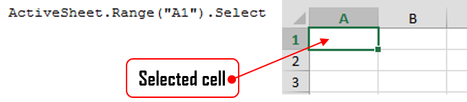
Working with Range variables

The Range is a separate object variable and can be declared as other variables. As the VBA Range is an object you need to use the Set statement:

Dim myRange as Range 
'...
Set myRange = Range("A1") 'Need to use Set to define myRange

The Range object defaults to your ActiveWorksheet. So beware as depending on your ActiveWorksheet the Range object will return values local to your worksheet:

Range("A1").Select
'...is the same as...
ActiveSheet.Range("A1").Select

You might want to define the Worksheet reference by Range if you want your reference values from a specifc Worksheet:

Sheets("Sheet1").Range("A1").Select 'Will always select items from Worksheet named Sheet1

The ActiveWorkbook is not same to ThisWorkbook. Same goes for the ActiveSheet. This may reference a Worksheet from within a Workbook external to the Workbook in which the macro is executed as Active references simply the currently top-most worksheet. Read more here

Range properties

The Range object contains a variety of properties with the main one being it’s Value and an the second one being its Formula.

A Range Value is the evaluated property of a cell or a range of cells. For example a cell with the formula =10+20 has an evaluated value of 20.
A Range Formula is the formula provided in the cell or range of cells. For example a cell with a formula of =10+20 will have the same Formula property.

'Let us assume A1 contains the formula "=10+20"

Debug.Print Range("A1").Value 'Returns: 30

Debug.Print Range("A1").Formula 'Returns: =10+20

Other Range properties include:
Work in progress

Worksheet Cells

A Worksheet Cells property is similar to the Range property but allows you to obtain only a SINGLE CELL, based on its row and column index. Numbering starts at 1:

The Cells property is in fact a Range object not a separate data type.
Excel facilitates a Cells function that allows you to obtain a cell from within the ActiveSheet, current top-most worksheet.

Cells(2,2).Select 'Selects B2
'...is the same as...
ActiveSheet.Cells(2,2).Select 'Select B2

Cells are Ranges which means they are not a separate data type:

Dim myRange as Range
Set myRange = Cells(1,1) 'Cell A1

Range Rows and Columns

As we all know an Excel Worksheet is divided into Rows and Columns. The Excel VBA Range object allows you to select single or multiple rows as well as single or multiple columns. There are a couple of ways to obtain Worksheet rows in VBA:

Getting an entire row or column

To get and entire row of a specified Range you need to use the EntireRow property. Although, the function’s parameters suggest taking both a RowIndex and ColumnIndex it is enough just to provide the row number. Row indexing starts at 1.
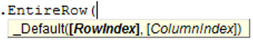To get and entire column of a specified Range you need to use the EntireColumn property. Although, the function’s parameters suggest taking both a RowIndex and ColumnIndex it is enough just to provide the column number. Column indexing starts at 1.

Range("B2").EntireRows(1).Hidden = True 'Gets and hides the entire row 2

Range("B2").EntireColumns(1).Hidden = True 'Gets and hides the entire column 2

The three properties EntireRow/EntireColumn, Rows/Columns and Row/Column are often misunderstood so read through to understand the differences.

Get a row/column of a specified range

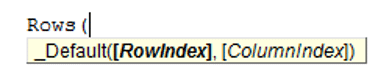If you want to get a certain row within a Range simply use the Rows property of the Worksheet. Although, the function’s parameters suggest taking both a RowIndex and ColumnIndex it is enough just to provide the row number. Row indexing starts at 1.
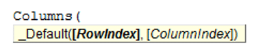Similarly you can use the Columns function to obtain any single column within a Range. Although, the function’s parameters suggest taking both a RowIndex and ColumnIndex actually the first argument you provide will be the column index. Column indexing starts at 1.

Rows(1).Hidden = True 'Hides the first row in the ActiveSheet
'same as
ActiveSheet.Rows(1).Hidden = True

Columns(1).Hidden = True 'Hides the first column in the ActiveSheet
'same as
ActiveSheet.Columns(1).Hidden = True

To get a range of rows/columns you need to use the Range function like so:

Range(Rows(1), Rows(3)).Hidden = True 'Hides rows 1:3
'same as
Range("1:3").Hidden = True
'same as 
ActiveSheet.Range("1:3").Hidden = True

Range(Columns(1), Columns(3)).Hidden = True 'Hides columns A:C
'same as
Range("A:C").Hidden = True
'same as 
ActiveSheet.Range("A:C").Hidden = True

Get row/column of specified range

The above approach assumed you want to obtain only rows/columns from the ActiveSheet – the visible and top-most Worksheet. Usually however, you will want to obtain rows or columns of an existing Range. Similarly as with the Worksheet Range property, any Range facilitates the Rows and Columns property.

Dim myRange as Range
Set myRange = Range("A1:C3")

myRange.Rows.Hidden = True 'Hides rows 1:3
myRange.Columns.Hidden = True 'Hides columns A:C

Set myRange = Range("C10:F20")
myRange.Rows(2).Hidden = True 'Hides rows 11
myRange.Columns(3).Hidden = True 'Hides columns E

Getting a Ranges first row/column number

Aside from the Rows and Columns properties Ranges also facilitate a Row and Column property which provide you with the number of the Ranges first row and column.

Set myRange = Range("C10:F20")

'Get first row number
Debug.Print myRange.Row 'Result: 10
'Get first column number
Debug.Print myRange.Column 'Result: 3

Converting Column number to Excel Column

This is an often question that turns up – how to convert a column number to a string e.g. 100 to “CV”.

Function GetExcelColumn(columnNumber As Long)
    Dim div As Long, colName As String, modulo As Long
    div = columnNumber: colName = vbNullString

    Do While div > 0
        modulo = (div - 1) Mod 26
        colName = Chr(65 + modulo) & colName
        div = ((div - modulo) / 26)
    Loop

    GetExcelColumn = colName
End Function

Range Cut/Copy/Paste

Cutting and pasting rows is generally a bad practice which I heavily discourage as this is a practice that is moments can be heavily cpu-intensive and often is unaccounted for.

Copy function

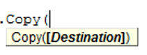The Copy function works on a single cell, subset of cell or subset of rows/columns.

'Copy values and formatting from cell A1 to cell D1
Range("A1").Copy Range("D1")

'Copy 3x3 A1:C3 matrix to D1:F3 matrix - dimension must be same
Range("A1:C3").Copy Range("D1:F3")

'Copy rows 1:3 to rows 4:6
Range("A1:A3").EntireRow.Copy Range("A4")

'Copy columns A:C to columns D:F
Range("A1:C1").EntireColumn.Copy Range("D1")

The Copy function can also be executed without an argument. It then copies the Range to the Windows Clipboard for later Pasting.

Cut function

The Cut function, similarly as the Copy function, cuts single cells, ranges of cells or rows/columns.

'Cut A1 cell and paste it to D1
Range("A1").Cut Range("D1")

'Cut 3x3 A1:C3 matrix and paste it in D1:F3 matrix - dimension must be same
Range("A1:C3").Cut Range("D1:F3")

'Cut rows 1:3 and paste to rows 4:6
Range("A1:A3").EntireRow.Cut Range("A4")

'Cut columns A:C and paste to columns D:F
Range("A1:C1").EntireColumn.Cut Range("D1")

The Cut function can be executed without arguments. It will then cut the contents of the Range and copy it to the Windows Clipboard for pasting.

Cutting cells/rows/columns does not shift any remaining cells/rows/columns but simply leaves the cut out cells empty

PasteSpecial function

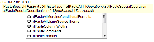The Range PasteSpecial function works only when preceded with either the Copy or Cut Range functions. It pastes the Range (or other data) within the Clipboard to the Range on which it was executed.

Syntax

The PasteSpecial function has the following syntax:

PasteSpecial( Paste, Operation, SkipBlanks, Transpose)

The PasteSpecial function can only be used in tandem with the Copy function (not Cut)

Parameters

Paste
The part of the Range which is to be pasted. This parameter can have the following values:

Parameter	Constant	Description
xlPasteSpecialOperationAdd	2	Copied data will be added with the value in the destination cell.
xlPasteSpecialOperationDivide	5	Copied data will be divided with the value in the destination cell.
xlPasteSpecialOperationMultiply	4	Copied data will be multiplied with the value in the destination cell.
xlPasteSpecialOperationNone	-4142	No calculation will be done in the paste operation.
xlPasteSpecialOperationSubtract	3	Copied data will be subtracted with the value in the destination cell.

Operation
The paste operation e.g. paste all, only formatting, only values, etc. This can have one of the following values:

Name	Constant	Description
xlPasteAll	-4104	Everything will be pasted.
xlPasteAllExceptBorders	7	Everything except borders will be pasted.
xlPasteAllMergingConditionalFormats	14	Everything will be pasted and conditional formats will be merged.
xlPasteAllUsingSourceTheme	13	Everything will be pasted using the source theme.
xlPasteColumnWidths	8	Copied column width is pasted.
xlPasteComments	-4144	Comments are pasted.
xlPasteFormats	-4122	Copied source format is pasted.
xlPasteFormulas	-4123	Formulas are pasted.
xlPasteFormulasAndNumberFormats	11	Formulas and Number formats are pasted.
xlPasteValidation	6	Validations are pasted.
xlPasteValues	-4163	Values are pasted.
xlPasteValuesAndNumberFormats	12	Values and Number formats are pasted.

SkipBlanks
If True then blanks will not be pasted.

Transpose
Transpose the Range before paste (swap rows with columns).

PasteSpecial Examples

'Cut A1 cell and paste its values to D1
Range("A1").Copy
Range("D1").PasteSpecial
 
'Copy 3x3 A1:C3 matrix and add all the values to E1:G3 matrix (dimension must be same)
Range("A1:C3").Copy 
Range("E1:G3").PasteSpecial xlPasteValues, xlPasteSpecialOperationAdd

Below an example where the Excel Range A1:C3 values are copied an added to the E1:G3 Range. You can also multiply, divide and run other similar operations.

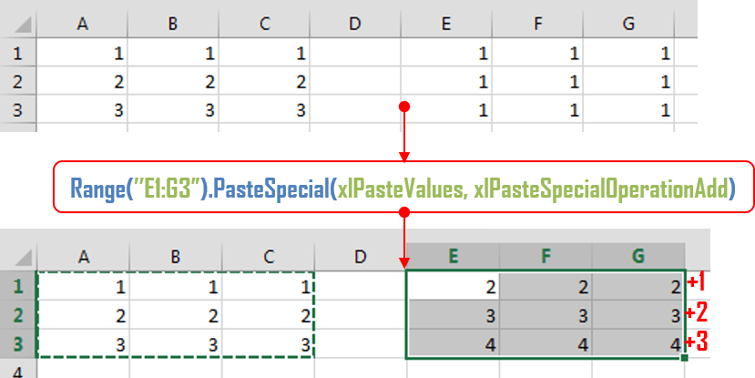
Paste

The Paste function allows you to paste data in the Clipboard to the actively selected Range. Cutting and Pasting can only be accomplished with the Paste function.

'Cut A1 cell and paste its values to D1
Range("A1").Cut
Range("D1").Select
ActiveSheet.Paste
 
'Cut 3x3 A1:C3 matrix and paste it in D1:F3 matrix - dimension must be same
Range("A1:C3").Cut 
Range("D1:F3").Select
ActiveSheet.Paste
 
'Cut rows 1:3 and paste to rows 4:6
Range("A1:A3").EntireRow.Cut 
Range("A4").Select
ActiveSheet.Paste
 
'Cut columns A:C and paste to columns D:F
Range("A1:C1").EntireColumn.Cut 
Range("D1").Select
ActiveSheet.Paste

Range Clear/Delete

The Clear function

The Clear function clears the entire content and formatting from an Excel Range. It does not, however, shift (delete) the cleared cells.

Range("A1:C3").Clear

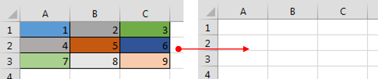
The Delete function

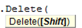The Delete function deletes a Range of cells, removing them entirely from the Worksheet, and shifts the remaining Cells in a selected shift direction.
Although the manual Delete cell function provides 4 ways of shifting cells. The VBA Delete Shift values can only be either be xlShiftToLeft or xlShiftUp.

'If Shift omitted, Excel decides - shift up in this case
Range("B2").Delete 

'Delete and Shift remaining cells left
Range("B2").Delete xlShiftToLeft  

'Delete and Shift remaining cells up
Range("B2").Delete xlShiftTop

'Delete entire row 2 and shift up
Range("B2").EntireRow.Delete

'Delete entire column B and shift left
Range("B2").EntireRow.Delete

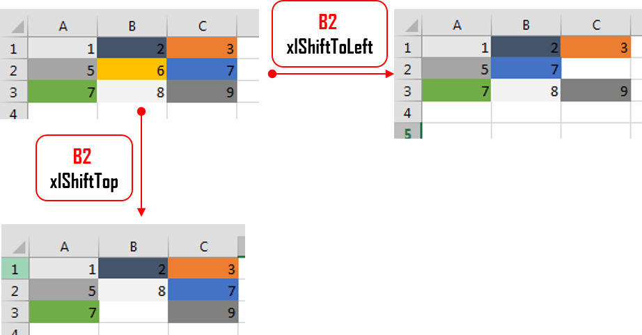
Traversing Ranges

Traversing cells is really useful when you want to run an operation on each cell within an Excel Range. Fortunately this is easily achieved in VBA using the For Each or For loops.

Dim cellRange As Range
    
For Each cellRange In Range("A1:C3")
  Debug.Print cellRange.Value
Next cellRange

Although this may not be obvious, beware of iterating/traversing the Excel Range using a simple For loop. For loops are not efficient on Ranges. Use a For Each loop as shown above. This is because Ranges resemble more Collections than Arrays. Read more on For vs For Each loops here

Traversing the UsedRange

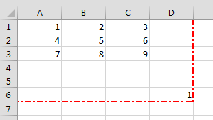Every Worksheet has a UsedRange. This represents that smallest rectangle Range that contains all cells that have or had at some point values. In other words if the further out in the bottom, right-corner of the Worksheet there is a certain cell (e.g. E8) then the UsedRange will be as large as to include that cell starting at cell A1 (e.g. A1:E8). In Excel you can check the current UsedRange hitting CTRL+END. In VBA you get the UsedRange like this:

ActiveSheet.UsedRange
'same as
UsedRange

You can traverse through the UsedRange like this:

Dim cellRange As Range
    
For Each cellRange In UsedRange
  Debug.Print "Row: " & cellRange.Row & ", Column: " & cellRange.Column
Next cellRange

The UsedRange is a useful construct responsible often for bloated Excel Workbooks. Often delete unused Rows and Columns that are considered to be within the UsedRange can result in significantly reducing your file size. Read also more on the XSLB file format here

Range Addresses

The Excel Range Address property provides a string value representing the Address of the Range.

Syntax

Below the syntax of the Excel Range Address property:

Address( [RowAbsolute], [ColumnAbsolute], [ReferenceStyle], [External], [RelativeTo] )

Parameters

RowAbsolute
Optional. If True returns the row part of the reference address as an absolute reference. By default this is True.

$D$10:$G$100 'RowAbsolute is set to True
$D10:$G100 'RowAbsolute is set to False

ColumnAbsolute
Optional. If True returns the column part of the reference as an absolute reference. By default this is True.

$D$10:$G$100 'ColumnAbsolute is set to True
D$10:G$100 'ColumnAbsolute is set to False

ReferenceStyle
Optional. The reference style. The default value is xlA1. Possible values:

Constant	Value	Description
xlA1	1	Default. Use xlA1 to return an A1-style reference
xlR1C1	-4150	Use xlR1C1 to return an R1C1-style reference

External
Optional. If True then property will return an external reference address, otherwise a local reference address will be returned. By default this is False.

$A$1 'Local
[Book1.xlsb]Sheet1!$A$1 'External

RelativeTo
Provided RowAbsolute and ColumnAbsolute are set to False, and the ReferenceStyle is set to xlR1C1, then you must include a starting point for the relative reference. This must be a Range variable to be set as the reference point.

Merged Ranges

Merged cells are Ranges that consist of 2 or more adjacent cells. To Merge a collection of adjacent cells run Merge function on that Range.

The Merge has only a single parameter – Across, a boolean which if True will merge cells in each row of the specified range as separate merged cells. Otherwise the whole Range will be merged. The default value is False.

Merge examples

To merge the entire Range:

'This will turn of any alerts warning that values may be lost
Application.DisplayAlerts = False

Range("B2:C3").Merge

This will result in the following:

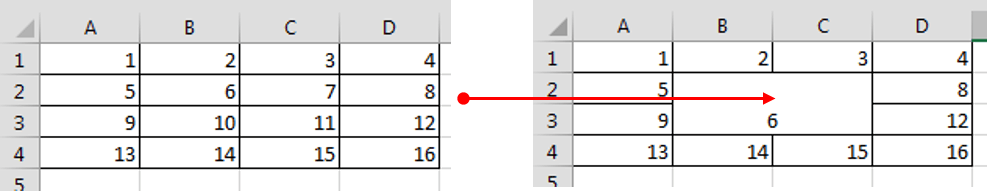
To merge just the rows set Across to True.

'This will turn of any alerts warning that values may be lost
Application.DisplayAlerts = False

Range("B2:C3").Merge True

This will result in the following:

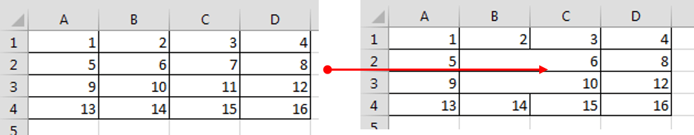
Remember that merged Ranges can only have a single value and formula. Hence, if you merge a group of cells with more than a single value/formula only the first value/formula will be set as the value/formula for your new merged Range

Checking if Range is merged

To check if a certain Range is merged simply use the Excel Range MergeCells property:

Range("B2:C3").Merge

Debug.Print Range("B2").MergeCells 'Result: True

The MergeArea

The MergeArea is a property of an Excel Range that represent the whole merge Range associated with the current Range. Say that $B$2:$C$3 is a merged Range – each cell within that Range (e.g. B2, C3..) will have the exact same MergedArea. See example below:

Range("B2:C3").Merge
Debug.Print Range("B2").MergeArea.Address 'Result: $B$2:$C$3

Named Ranges

Named Ranges are Ranges associated with a certain Name (string). In Excel you can find all your Named Ranges by going to Formulas->Name Manager. They are very useful when working on certain values that are used frequently through out your Workbook. Imagine that you are writing a Financial Analysis and want to use a common Discount Rate across all formulas. Just the address of the cell e.g. “A2”, won’t be self-explanatory. Why not use e.g. “DiscountRate” instead? Well you can do just that.

Creating a Named Range

Named Ranges can be created either within the scope of a Workbook or Worksheet:

Dim r as Range
'Within Workbook
Set r = ActiveWorkbook.Names.Add("NewName", Range("A1"))
'Within Worksheet
Set r = ActiveSheet.Names.Add("NewName", Range("A1"))

This gives you flexibility to use similar names across multiple Worksheets or use a single global name across the entire Workbook.

Listing all Named Ranges

You can list all Named Ranges using the Name Excel data type. Names are objects that represent a single NamedRange. See an example below of listing our two newly created NamedRanges:

Call ActiveWorkbook.Names.Add("NewName", Range("A1"))
Call ActiveSheet.Names.Add("NewName", Range("A1"))

Dim n As Name
For Each n In ActiveWorkbook.Names
  Debug.Print "Name: " & n.Name & ", Address: " & _
       n.RefersToRange.Address & ", Value: "; n.RefersToRange.Value
Next n

'Result:
'Name: Sheet1!NewName, Address: $A$1, Value:  1 
'Name: NewName, Address: $A$1, Value:  1

SpecialCells

SpecialCells are a very useful Excel Range property, that allows you to select a subset of cells/Ranges within a certain Range.

Syntax

The SpecialCells property has the following syntax:

SpecialCells( Type, [Value] )

Parameters

Type
The type of cells to be returned. Possible values:

Constant	Value	Description
xlCellTypeAllFormatConditions	-4172	Cells of any format
xlCellTypeAllValidation	-4174	Cells having validation criteria
xlCellTypeBlanks	4	Empty cells
xlCellTypeComments	-4144	Cells containing notes
xlCellTypeConstants	2	Cells containing constants
xlCellTypeFormulas	-4123	Cells containing formulas
xlCellTypeLastCell	11	The last cell in the used range
xlCellTypeSameFormatConditions	-4173	Cells having the same format
xlCellTypeSameValidation	-4175	Cells having the same validation criteria
xlCellTypeVisible	12	All visible cells

Value
If Type is equal to xlCellTypeConstants or xlCellTypeFormulas this determines the types of cells to return e.g. with errors.

Constant	Value
xlErrors	16
xlLogical	4
xlNumbers	1
xlTextValues	2

SpecialCells examples

Get Excel Range with Constants

This will return only cells with constant cells within the Range C1:C3:

For Each r In Range("A1:C3").SpecialCells(xlCellTypeConstants)
  Debug.Print r.Value
Next r

Search for Excel Range with Errors

For Each r In ActiveSheet.UsedRange.SpecialCells(xlCellTypeFormulas, xlErrors)
  Debug.Print r.Address
Next r

Источник

Hide UnHide Rows in Excel Worksheet using VBA

17 Comments

LS
July 24, 2015 at 10:23 AM — Reply

In case I want to hide a row with condition…… for eg. I have a data base with some columns having text and some having numbers. If value in one of the columns becomes 0 or a negative number or a text then that row should get hidden.

could you please automate such a task in excel ?

thanks.
PNRao
July 25, 2015 at 3:04 AM — Reply

Hi Lata,

I have updated the post with number of examples with criteria.
Please check now:Hiding Rows with Criteria in Excel Worksheet using VBA – Example File
Thanks-PNRao!
Ben
August 7, 2015 at 8:00 PM — Reply

I tried to apply the same principle to columns with the conditions in row 1, but it can’t run.
Maybe someone knows what I need to fix in the script below :
Thanks!

LastColumn = “EZ” ‘Let’s say I have columns until “EZ” in the report
For i = “A” To LastColumn ‘I want to loop through each column and check for required criteria

‘to hide all the columns with the values as 0 in Row 1
If Range(1 & i) = 0 Then Column(i).EntireColumn.Hidden = True

Next
PNRao
August 8, 2015 at 3:25 PM — Reply
Ben
August 11, 2015 at 7:21 PM — Reply

Awesome!! Works like a charm,

Thanks again!
PNRao
August 11, 2015 at 11:51 PM — Reply

Welcome! I’m glad it worked. Thanks-PNRao
patrick
December 7, 2015 at 5:40 PM — Reply

My desire is to specific cells. I have checkboxes and command buttons sprinkled throughout the worksheet. What I like to do is to hide the cells containing these form types. Maybe I have to redesign my worksheet to have all these buttons and boxes either all in a row or a column and hide the row/column. Have not had much luck with this. Can you help please?
amina1987
March 9, 2016 at 4:16 PM — Reply

good morning.
thank you for this very usefull topic.

for my work (for 2400 workbooks) i need to hide specific rows without openning the workbooks. is that possible? please help
Hey Valli,

This is my first attempt to actually write a Macro, and looks like I am stuck (Terribly Stuck)

Here is what I am trying to achieve:
I have a “Input” sheet which is linked (Via Vlookups in C:C) to 8-10 other worksheets (containing rates of materials). On a daily basis I have to insert the quantities (in Column D:D) next to the rates in the “Input” Sheet to multiply it with the corresponding rates to arrive at the total amount (in Column E:E) eventually.
The issue is I have to hide the materials (Entire Rows) I do not use in the Input sheet as well as the other reference sheets. Is there any way a macro can be written to help me?
Guy
May 9, 2016 at 4:27 PM — Reply

HI PNRao,

Thanks for the great poste it really helped me, how would i loop this macro round to unhide the hidden rows when the box is unchecked?

Thanks
SANDIP DAVE
January 3, 2017 at 8:01 PM — Reply

I have a worksheet with live data of stock value, high, low in Column A3:A103, B3:B103, C3:C103 respectively and other formula in other columns and that updates every few seconds.
I would like to see only rows where below conditions is fulfilled and hide all other rows to filter out stocks.
Condition 1: =AND(A3=B3,A3>=L3,A3<=K3,A30)
Condition 2 =AND(A3=C3,A3>=S3,A3<=R3,A30)
Above condition is for example of Raw No.3 and which I am using for conditional formatting.
Kindly help to provide VBA codes for this.
Skup
June 26, 2017 at 11:52 AM — Reply

Greetings,

How would someone show/hide rows in a 2nd range based upon the visibility of rows in a filtered range?

For example, if rows 5 through 20 are autofiltered by some criteria such that at a given state only rows 6, 8. 12. and 16 through 18 are visible, how could someone then show the matching rows in the range of rows from 105 through 120, so that along with rows 6, 8. 12. and 16 through 18 being visible by filtering; rows 106, 108, 112, 116, 117, and 118 are visible, while rows 105, 107, 109, 110, 11, 113, 114, 115, 119, and 120 are hidden?

How can this be triggered by the setting and resetting of the autofilter on the filtered range?
Orlando
March 21, 2019 at 8:18 AM — Reply

How I can to hide Rows (A4:A6), and unhide Rows (A1:A3) in same time?
Carlos
February 4, 2020 at 8:42 PM — Reply

Hi Everyone,

I need help to write a VB macro which allows me to use a Hide Rows/Unhide Rows button(s) using a zero value or blank range in Column D. I’ve tried taking various examples from here and other sites to try to help but either I’m doing something wrong (most likely) or the code wasn’t correct for my requirements in the first place!

Can anyone help please, I’m so lost!!!
Jasper
April 11, 2020 at 12:42 AM — Reply

In your first example you say you’re hiding rows 5-8
IN the code you say Hide Rows 22-25
with the code set to 5:8

Just got me confused
Eugene Van Loggerenberg
May 20, 2020 at 4:21 PM — Reply

Good day

I am just starting out and have zero VBA experience.
I have been able to create a button and link it to VBA and that part works.
Using the “Hide all rows with the values as 0 in Column A” I am having problems getting it to work.

Assistance would be much appreciated.

Regards Eugene
PNRao
September 6, 2020 at 8:55 PM — Reply

Effectively Manage Your
Projects and Resources

With Our Professional and Premium Project Management Templates!

ANALYSISTABS.COM provides free and premium project management tools, templates and dashboards for effectively managing the projects and analyzing the data.

We’re a crew of professionals expertise in Excel VBA, Business Analysis, Project Management. We’re Sharing our map to Project success with innovative tools, templates, tutorials and tips.

Project Management

Excel VBA

Download Free Excel 2007, 2010, 2013 Add-in for Creating Innovative Dashboards, Tools for Data Mining, Analysis, Visualization. Learn VBA for MS Excel, Word, PowerPoint, Access, Outlook to develop applications for retail, insurance, banking, finance, telecom, healthcare domains.

Page load link

Go to Top

Источник

Довольно часто появляется необходимость в Excel скрывать или отображать строки или столбцы. Особенно это актуально, когда на листе размещается очень много информации и часть из них является вспомогательной и требуется не всегда и тем самым загромождает пространство, ухудшая восприятие. Если это приходится делать часто, то делать это с помощью меню неудобно, особенно если приходится скрывать и отображать разные столбцы и строки.

Для существенного удобства можно написать простенький макрос, привязав его к кнопке и делать это одним щелком мыши.

Вот так выглядят простые примеры, с помощью которых Вы без труда сможете скрывать или отображать строки и столбцы с помощью VBA

Пример 1: Скрыть строку 2 в Excel

Sub HideString() ‘Это название макроса

Rows(2).Hidden = True

End Sub

Пример 2: Скрыть несколько строк в Excel (строку 3-5)

Sub HideStrings()

Rows(«3:5»).Hidden = True

End Sub

Пример 3: Скрыть столбец 2 в Excel

Sub HideCollumn()

Columns(2).Hidden = True

End Sub

Пример 4: Скрытие нескольких столбцов в Excel

Sub HideCollumns()

Columns(«E:F»).Hidden = True

End Sub

Пример 5: Скрытие строки по имени ячейки в Excel

Sub HideCell()

Range(«Возможности Excel»).EntireRow.Hidden = True

End Sub

Пример 6: Скрытие нескольких строк по адресам ячеек

Sub HideCell()

Range(«B3:D4»).EntireRow.Hidden = True

End Sub

Пример 7: Скрытие столбца по имени ячейки

Sub HideCell()

Range(«Возможности Excel»).EntireColumn.Hidden = True

End Sub

Пример 8: Скрытие нескольких столбцов по адресам ячеек

Sub HideCell()

Range(«C2:D5»).EntireColumn.Hidden = True

End Sub

Как видите процесс автоматического скрытия строк и столбцов очень прост, а применений данному приему огромное множество.

Для того, чтобы отобразить строки и столбцы в Excel вы можете воспользоваться этими же макросами, но вместе True необходимо указать False

Например, макрос для того, чтобы отобразить строку 2 будет выглядеть следующим образом:

Sub ViewString()

Rows(2).Hidden = False

End Sub

Надеемся, что данная статья была полезна вам и ответила на вопрос: как скрыть или отобразить строки и столбцы в Excel с помощью VBA

Спасибо за внимание.

Источник

Синтаксис

Примечание

Примеры кода с Range.Hidden

Пример 1

Пример 2

Пример 3

Пример 4

Hide / Unhide Columns & Rows

Hide Columns or Rows

Hide Columns

Hide Rows

Unhide Columns or Rows

Unhide All Columns or Rows

VBA Coding Made Easy

VBA Code Examples Add-in

Excel VBA Hide Or Unhide Columns And Rows: 16 Macro Code Examples You Can Use Right Now

Excel VBA Constructs To Hide Rows Or Columns

Hide Or Unhide With The Range.Hidden Property

How To Hide Rows Or Columns With The Range.Hidden Property

How To Unhide Rows Or Columns With The Range.Hidden Property

Specify Row Or Column To Hide Or Unhide Using VBA

Worksheet.Range Property

Syntax #1: expression.Range(Cell)

Syntax #2: expression.Range(Cell1, Cell2)

How To Refer To An Entire Row Or Column With the Worksheet.Range Property

Worksheet.Cells Property

Worksheet.Columns Property

Worksheet.Rows Property

Range.EntireRow Property

Range.EntireColumn Property

Excel VBA Code Examples To Hide Columns

VBA Code Example #1: Hide A Column

VBA Code Example #2: Hide Several Contiguous Columns

VBA Code Example #3: Hide Several Non-Contiguous Columns

Excel VBA Code Examples To Hide Rows

VBA Code Example #4: Hide A Row

VBA Code Example #5: Hide Several Contiguous Rows

VBA Code Example #6: Hide Several Non-Contiguous Rows

Excel VBA Code Examples To Unhide Columns

VBA Code Example #7: Unhide A Column

VBA Code Example #8: Unhide Several Contiguous Columns

VBA Code Example #9: Unhide Several Non-Contiguous Columns

VBA Code Examples #10 And #11: Unhide All Columns In A Worksheet

VBA Code Example #10: Unhide All Columns In A Worksheet Using The Worksheet.Cells Property

VBA Code Example #11: Unhide All Columns In A Worksheet Using The Worksheet.Columns Property

Excel VBA Code Examples To Unhide Rows

VBA Code Example #12: Unhide A Row

VBA Code Example #13: Unhide Several Contiguous Rows

VBA Code Example #14: Unhide Several Non-Contiguous Rows

VBA Code Examples #15 And #16: Unhide All Columns In A Worksheet

VBA Code Example #15: Unhide All Rows In A Worksheet Using The Worksheet.Cells Property

VBA Code Example #16: Unhide All Rows In A Worksheet Using The Worksheet.Rows Property

Conclusion

Hide Columns or Rows

Hide Columns

Hide Rows

Unhide Columns or Rows

Unhide All Columns or Rows

VBA Coding Made Easy

Range object (Excel)

Remarks

Example

Methods

Properties

See also

Excel VBA Constructs To Hide Rows Or Columns

Hide Or Unhide With The Range.Hidden Property

How To Hide Rows Or Columns With The Range.Hidden Property

How To Unhide Rows Or Columns With The Range.Hidden Property

Specify Row Or Column To Hide Or Unhide Using VBA

Worksheet.Range Property

Syntax #1: expression.Range(Cell)

Syntax #2: expression.Range(Cell1, Cell2)

How To Refer To An Entire Row Or Column With the Worksheet.Range Property

Worksheet.Cells Property

Worksheet.Columns Property

Worksheet.Rows Property

Range.EntireRow Property

Range.EntireColumn Property

VBA Code Example #1: Hide A Column