
You can control the display of formulas in the following ways:
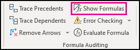
Click on Formulas and then click on Show Formulas to switch between displaying formulas and results.
Press CTRL + ` (grave accent).
Note: This procedure also prevents the cells that contain the formula from being edited.
-
Select the range of cells whose formulas you want to hide. You can also select nonadjacent ranges or the entire sheet.
-
Click Home > Format > Format Cells.
-
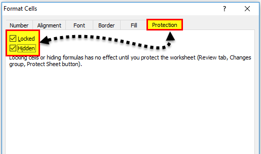
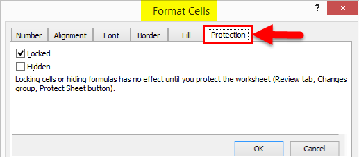
On the Protection tab, select the Hidden check box.
-
Click OK.
-
Click Review > Protect Sheet.
-
Make sure the Protect worksheet and contents of locked cells check box is selected, and then click OK.
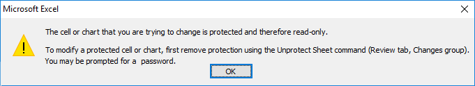
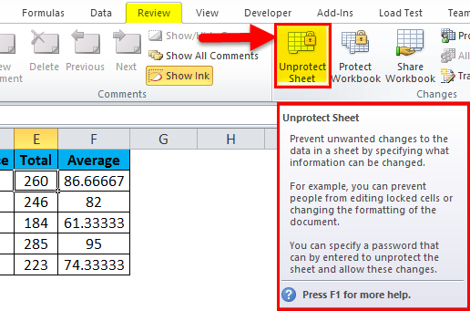
Click the Review tab, and then click Unprotect Sheet. If the Unprotect Sheet button is unavailable, turn off the Shared Workbook feature first.
If you don’t want the formulas hidden when the sheet is protected in the future, right-click the cells, and click Format Cells. On the Protection tab, clear the Hidden check box.
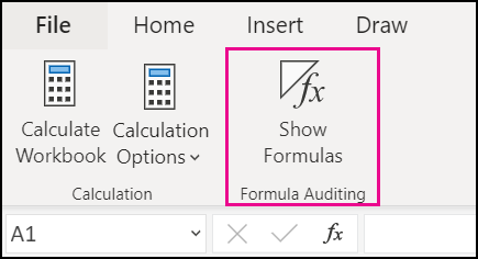
Click on Formulas and then click on Show Formulas to switch between displaying formulas and results.
When you share a normal Excel file with others, they are able to see and edit everything that the Excel file has.
If you don’t want them to change anything, you have the option to either protect the entire worksheet/workbook or protect certain cells that have important data (that you don’t want the user to mess up).
But even when you protect the worksheet, the end-user can still click on a cell and see the formula that’s used for calculations.
If you want to hide the formula so that the users cannot see those, you can do that as well.
In this exact tutorial, I will show you how to hide formulas in Excel in a protected worksheet (so that’s it’s not visible to the user).
So let’s get started!
How to Hide All Formulas in Excel
When you have a formula in a cell, a user can see the formula in two ways:
- By double-clicking on the cells and getting into the edit mode
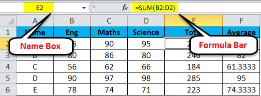
- By selecting the cell and seeing the formula in the formula bar
When you hide the formulas (as we’ll soon see how), the users won’t be able to edit the cell as well as not be able to see the formula in the formula bar.
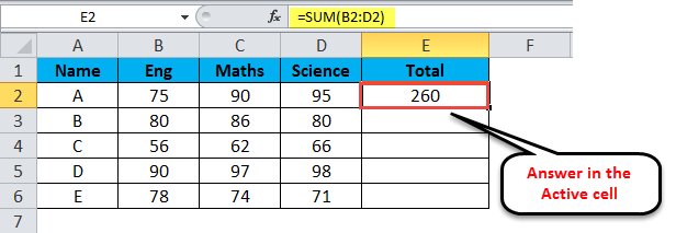
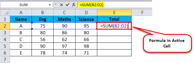
Suppose you have a data set as shown below where you have the formula in column D.

Below are the steps to hide all the formulas in column D:
- Select the cells in column D that have the formula that you want to hide

- Click the ‘Home’ tab

- In the ‘Number’ group, click on the dialog box launcher (it’s the small tilted arrow icon at the bottom right of the group)

- In the ‘Format Cells’ dialog box that opens up, click the ‘Protection’ tab

- Check the Hidden option

- Click OK
- Click the Review tab in the ribbon

- In the Protect group, click on the Protect Sheet option

- In the Protection dialog box, enter the password that would be needed if you want to unlock the worksheet (in case you don’t want to apply a password, you can leave this blank)

- Click OK


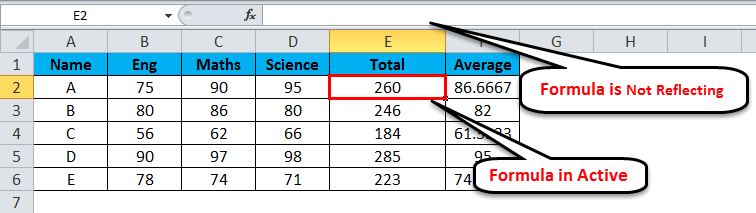
The above steps would protect the entire worksheet in such a way that if you click on a cell that has a value you would see the value in the formula bar, but if you click on a cell that has a formula, no formula would be shown in the formula bar.
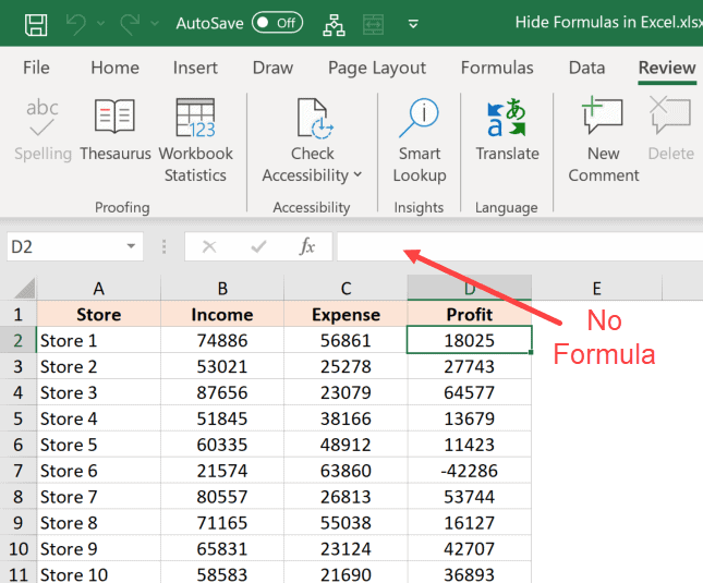
And since the worksheet is protected, you would not be able to double-click on the cell and get into the edit mode (so the formula is hidden that way as well).
While this method works fine, you need to know that the sheets/cells that are protected in Excel can easily be unlocked by the user.
Any tech-savvy user can easily break into your protected workbooks (a simple Google search will give them multiple ways to break the protected worksheet). It’s not straight-forward, but it’s not too hard.
But if you’re working with less tech-savvy users, adding a password should be enough.
Also read: How to Lock Formulas in Excel
How to Only Hide Formulas in Excel (And Keep Rest of the Cells Editable)
In the above method, I showed you how to protect the entire worksheet (including the cells that have don’t have a formula in it).
But what if you don’t want to protect the entire worksheet? What if you only want to protect the cells that have formulas and hide these formulas from the user.
This could be the case when you want the users to input data (such as in a data entry form) but not be able to edit the formula or see it.
This can easily be done as well.
Unlike the previous method, where we protected all the cells in the worksheet, in this method we would only select the cells that have the formulas and protect these cells.
The remaining of the worksheet would remain open for the user to edit.
Suppose you have a data set as shown below where you only want to protect the formulas in column D (which has formulas).
For a cell to be protected, it needs to have the ‘Locked’ property enabled, as well as the protection enabled from the ribbon. Only when both of these happen does a cell truly becomes locked (i.e., can’t be edited).
This also means that if you disable the lock property for a few cells, these could still be edited after you protect the worksheet.
We will use this concept where we will disable the locked property for all the cells except the ones that have formulas in it.
Let’s see how to do this.
Step 1 – Disable the Lock Property for all the Cells
So, we first need to disable the Locked property for all the cells (so that these can’t be protected)
Below are the steps to do this:
- Select all the cells in the worksheet (you can do this by clicking on the gray triangle at the top left part of the sheet).

- Click the Home tab
- In the Number group, click on the dialog box launcher
- In the Format cells dialog box, click on the ‘Protection’ tab
- Uncheck the Locked option

- Click Ok


The above steps have disabled the locked property for all the cells in the worksheet.
Now, even if I go and protect the sheet using the option in the ribbon (Review >> Protect Sheet), the cells would not be completely locked and you can still edit the cells.
Step 2 – Enable the Locked and Hidden Property only for Cells with Formulas
To hide the formula from all the cells in the worksheet, I now need to somehow identify the cells that have the formula and then lock these cells.
And while locking these cells, I would make sure that the formula is hidden from the formula bar as well.
Below are the steps to hide formulas:
- Select all the cells in the worksheet (you can do this by clicking on the gray triangle at the top left part of the sheet).
- Click the Home tab
- In the editing group, click on the Find & Select option

- Click on the ‘Go-To Special’ option.

- In the Go To Special dialog box, click on the Formulas option. This will select all the cells that have a formula in it

- With the cells with formulas selected, hold the Control key and then press the 1 key (or the Command key and the 1 key if using Mac). This will open the Number Format dialog box
- Click on the ‘Protection’ tab
- Make sure ‘Locked’ and ‘Hidden’ options are checked

- Click Ok


Step 3 – Protecting the Worksheet
In the process so far, the Locked property is disabled for all the cells except the ones that have a formula in it.
So now, if I protect the entire worksheet, only those cells would be protected that have a formula (as you need the Locked property to be enabled to truly lock a cell).
Here are the steps to do this:
- Click the Review tab
- In the Protect group, click on the ‘Protect Sheet’ option
- In the Protect Sheet dialog box, enter the password (optional)
- Click Ok
The above steps would lock only those cells that have a formula in it and at the same time hide the formula from the users.
The users won’t be able to double-click and get into the edit mode as well as see the formula in the formula bar.
How to Hide Formulas Without Protecting the Worksheet
If you’re wondering whether you can hide the formulas in Excel without protecting the sheet, unfortunately, you can’t.
While you can get this done by using a complex VBA code, it would be unreliable and can lead to other issues. Here is an article that shares such a code (use it if you really really can’t do without it)
As of now, the only way to hide the formulas in Excel is to protect the sheet and also make sure that the hidden properties enabled for the cells that have the formula.
I hope you found this tutorial useful.
You may also like the following Excel tutorials:
- How to Lock Cells in Excel
- How to Hide a Worksheet in Excel (that can not be unhidden)
- How to Unhide COLUMNS in Excel
- How to Unhide Sheets in Excel
- How to Hide or Show Formula Bar in Excel?
Содержание
- Способы спрятать формулу
- Способ 1: скрытие содержимого
- Способ 2: запрет выделения ячеек
- Вопросы и ответы

Иногда при создании документа с расчетами пользователю нужно спрятать формулы от чужих глаз. Прежде всего, такая необходимость вызвана нежеланием юзера, чтобы посторонний человек понял структуру документа. В программе Эксель имеется возможность скрыть формулы. Разберемся, как это можно сделать различными способами.
Способы спрятать формулу
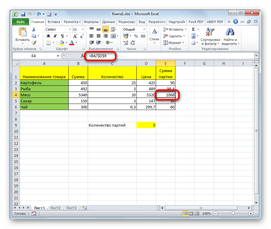
Ни для кого не секрет, что если в ячейке таблицы Excel имеется формула, то её можно увидеть в строке формул просто выделив эту ячейку. В определенных случаях это является нежелательным. Например, если пользователь хочет скрыть информацию о структуре вычислений или просто не желает, чтобы эти расчеты изменяли. В этом случае, логичным действием будет скрыть функцию.
Существует два основных способа сделать это. Первый из них представляет собой скрытие содержимого ячейки, второй способ более радикальный. При его использовании налагается запрет на выделение ячеек.
Способ 1: скрытие содержимого
Данный способ наиболее точно соответствует задачам, которые поставлены в этой теме. При его использовании только скрывается содержимое ячеек, но не налагаются дополнительные ограничения.
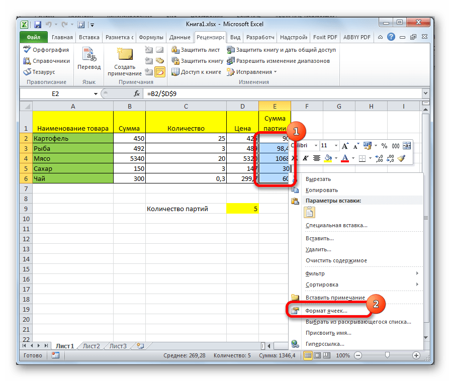
- Выделяем диапазон, содержимое которого нужно скрыть. Кликаем правой кнопкой мыши по выделенной области. Открывается контекстное меню. Выбираем пункт «Формат ячеек». Можно поступить несколько по-другому. После выделения диапазона просто набрать на клавиатуре сочетание клавиш Ctrl+1. Результат будет тот же.
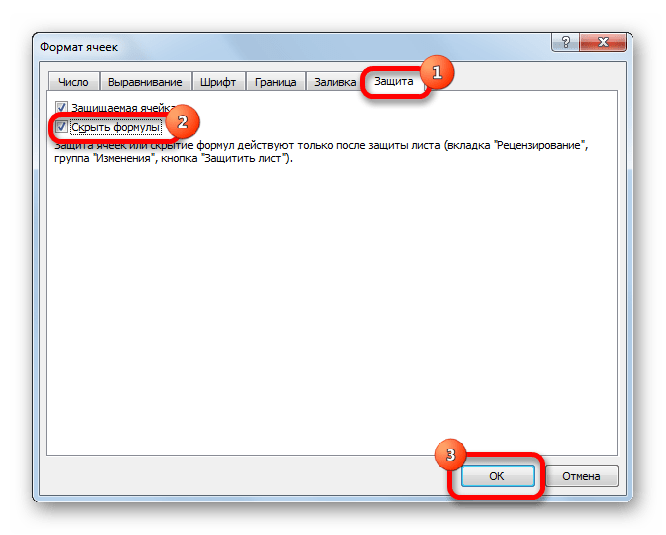
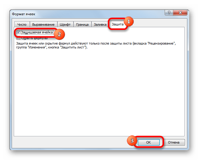
- Открывается окно «Формат ячеек». Переходим во вкладку «Защита». Устанавливаем галочку около пункта «Скрыть формулы». Галочку с параметра «Защищаемая ячейка» можно снять, если вы не планируете блокировать диапазон от изменений. Но, чаще всего, защита от изменений является как раз основной задачей, а скрытие формул – дополнительной. Поэтому в большинстве случаев обе галочки оставляют активными. Жмем на кнопку «OK».
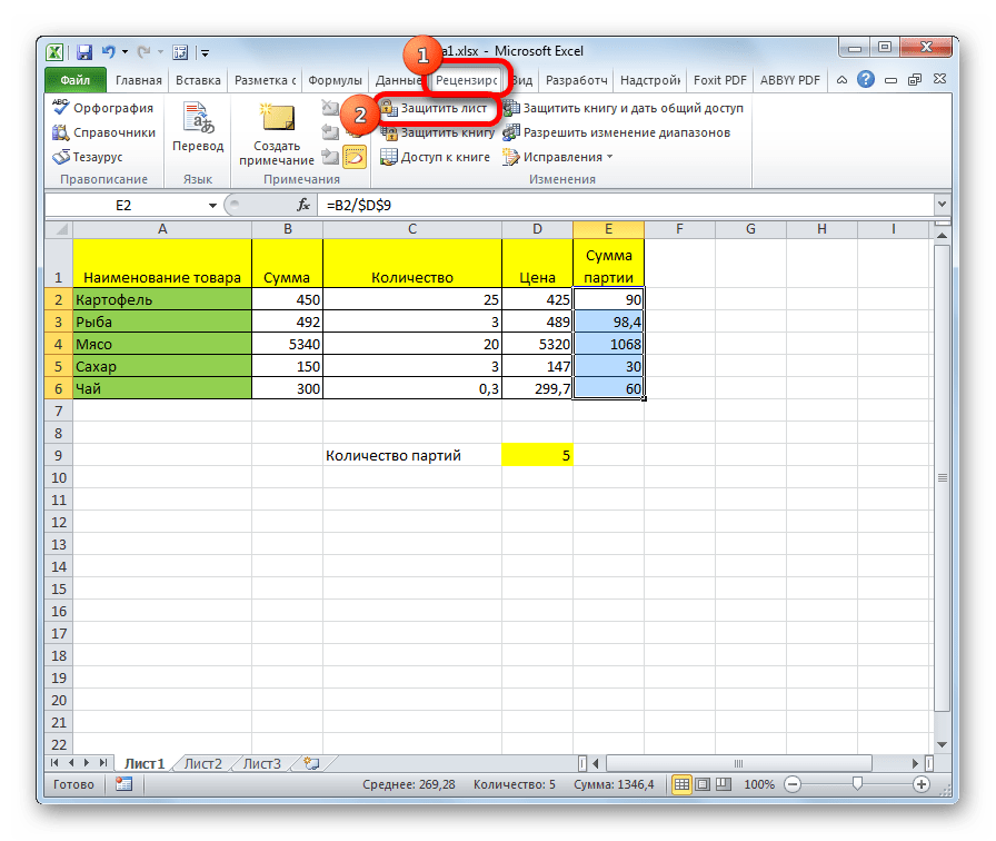
- После того, как окно закрыто, переходим во вкладку «Рецензирование». Жмем на кнопку «Защитить лист», расположенную в блоке инструментов «Изменения» на ленте.
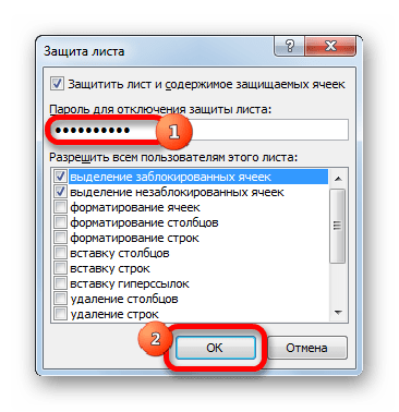
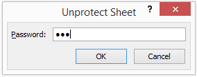
- Открывается окно, в поле которого нужно ввести произвольный пароль. Он потребуется, если вы захотите в будущем снять защиту. Все остальные настройки рекомендуется оставить по умолчанию. Затем следует нажать на кнопку «OK».
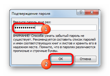
- Открывается ещё одно окно, в котором следует повторно набрать ранее введенный пароль. Это сделано для того, чтобы пользователь, вследствии введения неверного пароля (например, в измененной раскладке), не утратил доступ к изменению листа. Тут также после введения ключевого выражения следует нажать на кнопку «OK».
После этих действий формулы будут скрыты. В строке формул защищенного диапазона при их выделении ничего отображаться не будет.

Способ 2: запрет выделения ячеек
Это более радикальный способ. Его применение налагает запрет не только на просмотр формул или редактирование ячеек, но даже на их выделение.
- Прежде всего, нужно проверить установлена ли галочка около параметра «Защищаемая ячейка» во вкладке «Защита» уже знакомого по предыдущему способу нам окна форматирования выделенного диапазона. По умолчанию этот компонент должен был включен, но проверить его состояние не помешает. Если все-таки в данном пункте галочки нет, то её следует поставить. Если же все нормально, и она установлена, тогда просто жмем на кнопку «OK», расположенную в нижней части окна.
- Далее, как и в предыдущем случае, жмем на кнопку «Защитить лист», расположенную на вкладке «Рецензирование».
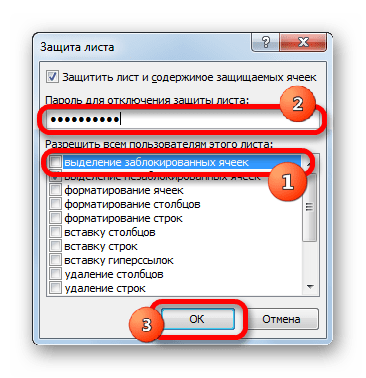
- Аналогично с предыдущим способом открывается окно введения пароля. Но на этот раз нам нужно снять галочку с параметра «Выделение заблокированных ячеек». Тем самым мы запретим выполнение данной процедуры на выделенном диапазоне. После этого вводим пароль и жмем на кнопку «OK».
- В следующем окошке, как и в прошлый раз, повторяем пароль и кликаем по кнопке «OK».

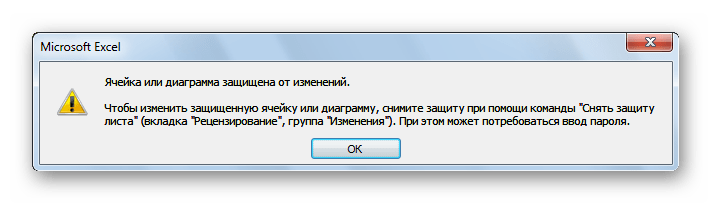
Теперь на выделенном ранее участке листа мы не просто не сможем просмотреть содержимое функций, находящихся в ячейках, но даже просто выделить их. При попытке произвести выделение будет появляться сообщение о том, что диапазон защищен от изменений.
Итак, мы выяснили, что отключить показ функций в строке формул и непосредственно в ячейке можно двумя способами. При обычном скрытии содержимого скрываются только формулы, как дополнительную возможность можно задать запрет их редактирования. Второй способ подразумевает наличие более жестких запретов. При его использовании блокируется не только возможность просмотра содержимого или его редактирования, но даже выделения ячейки. Какой из этих двух вариантов выбрать зависит, прежде всего, от поставленных задач. Впрочем, в большинстве случаев, первый вариант гарантирует достаточно надежную степень защиты, а блокировка выделения зачастую бывает излишней мерой предосторожности.
Еще статьи по данной теме:
Помогла ли Вам статья?
How to Hide Formulas in Excel?
Hiding formulas in Excel is a method when we do not want them to be displayed in the formula bar when we click on a cell with formulas. We can format the cells, check the hidden checkbox, and then protect the worksheet. It will prevent the formula from displaying in the “Formula” tab. Only the result of the formula will be visible.
Table of contents
- How to Hide Formulas in Excel?
- 13 Easy Steps to Hide Formula in Excel (with Example)
- Things to Remember
- Recommended Articles
13 Easy Steps to Hide Formula in Excel (with Example)
Let us understand the steps to hide formulas in Excel with examples.
You can download this Hide Formula Excel Template here – Hide Formula Excel Template
Step 1:
Following are the 13 steps that we can use to hide formulas in Excel:
- First, we must select the entire worksheet by pressing the shortcut key “Ctrl + A.”

- Now, on any cell, right-click and select “Format Cells” or press “Ctrl + 1.”

- Once the above option is selected, it may open the below dialog box and select “Protection.”

- Once the “Protection” tab is selected, uncheck the “Locked” option.
As a result, this will unlock all the cells in the worksheet. Remember, this may unlock the cells in the active worksheet in all the remaining worksheets. It remains locked only.
- If we observe as soon as we unlock the cells, Excel will notify us of an error as “Unprotected Formula.”

- Select only the formula cells and lock them. For example, we have three formulas in the worksheet, and we selected all three.

- Now, we must open the “Format Cells, select the “Protection” tab, and check the “Locked” and “Hidden” options.

Note: If we have many formulas in the Excel worksheet, we want to select each one of them, then we need to follow the below steps.
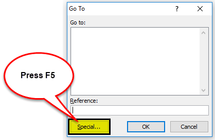
- Now, press the F5 (shortcut key to “Go to Special”) and select “Special.”

- Consequently, this will open up the below dialog box. Select “Formulas” and click “OK.” It would select all the formula cells in the worksheet.

Now, it has selected all the formula cells in the entire worksheet.
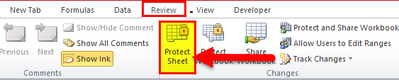
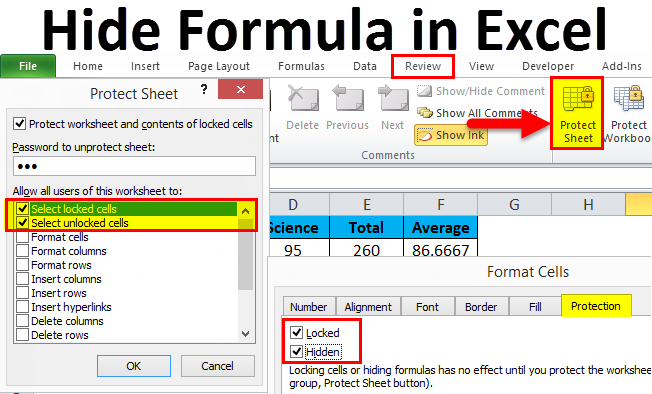
- Protect the sheet once the formula cells are selected, locked, and hidden. Then, go to the “Review” tab and “Protect Sheet.”

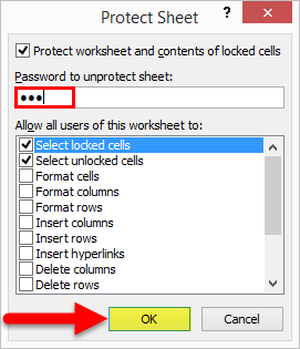
- Click on the “Protect Sheet” in Excel, and the dialog box may open up. Select only “Select locked cells” and “Select unlocked cells.” Type the password carefully because we cannot edit those cells if we forget the password.

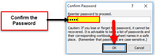
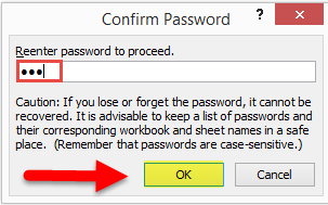
- Click on the “OK” button. It will again ask us to confirm the password. Enter the same password again.

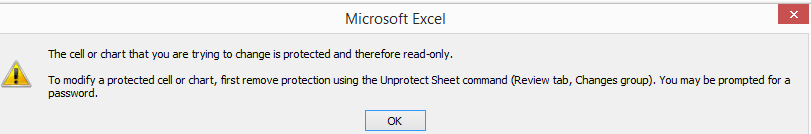
- Click on the “OK.” Now, our Excel formulas are locked and protected with a password. Suppose we cannot edit the password without the password. Then, if we try editing the formula, Excel will show the below warning message for us. Also, the formula bar does not show anything.


Things to Remember
- The most common way of hiding the formulas is by locking the particular cell and password protecting the worksheet.
- The first basic thing we need to do is “unlock all the cells in the active worksheet.” You must be wondering why we need to unlock all the cells in the worksheet where we did not even start the process of locking the cells in the worksheet.
- We need to unlock first by default. Then, Excel turns on excel Locked cellIn Excel, cells are locked to protect them from unwanted editing, deleting, and overwriting. Locking cells is specifically beneficial in cases where an excel worksheet needs to be shared with several colleagues.read more. However, we can still edit and manipulate the cells because we have not yet password-protected the sheet.
- We can open the “Go to Special” dialog box by pressing the “F5” shortcut.
- We must use the “Ctrl + 1” as the shortcut key to open the formatting options.
- Remember the password carefully. Otherwise, we cannot unprotect the worksheet.
- Only the password known person can edit the formulas.
Recommended Articles
This article has been a guide to Hide Formula in Excel. Here, we discuss how to hide formulas in Excel using the “Protection” tab to lock the cell and practical examples. You may learn more about Excel from the following articles: –
- Shortcut to Hide in Excel
- Unhide Sheets in Excel
- VBA Hide Columns
- How to Unhide Columns in Excel?
Home / Excel Formulas / How to Hide Formula in Excel
It happens sometimes you send Excel files to others and they made some changes to formulas. Or, sometimes you simply don’t want to show the formula to others.
Hiding a formula is a simple way to do this so that others can’t able to see which formula you have used and how they get calculated.
Now the question is, how can we hide the formula in a cell in Excel?
But before we do that let’s be clear on this point that there are two ways to see a formula from a cell, first, by editing a cell, and second, from the formula bar.
Is there any way you can use to prevent both things? Yes, it’s there. In Excel, there is a simple way for this, and today, I’d like to share with you this simple trick.
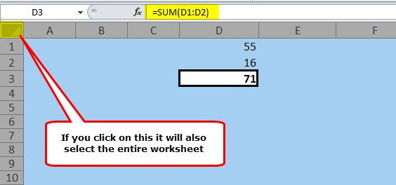
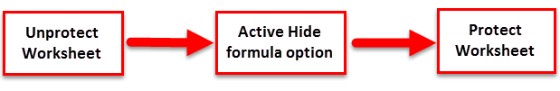
Step 1: Un-Protect Worksheet
At this point when you click on a cell, it shows you the entire formula in the formula bar.

- First of all, you need to make sure that your worksheet is unprotected.
- For this, go to the review tab and protect the group.
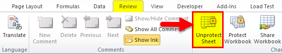
- If you find an “Unprotect Worksheet” button there, that means your worksheet is protected and you need to unprotect it.

- Click on that button to unprotect it.
If you have the “Protect Sheet” button there that means your worksheet is unprotected. In that case, skip the above steps and start from here.
Step 2: Activate the Hide Formula Option
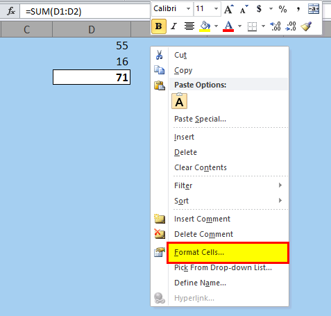
- Now, select the cell or range of cells, or select all the non-contiguous cells where you want to hide formulas.
- After that, right-click and select the format cells option.

- From the format cells option, go to the Protection tab.
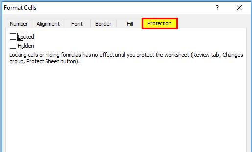
- In the protection tab, you have two checkboxes to mark, the first is locked and the second is hidden.
- Mark both of them and click OK.

These options which you have checked solve both of the problems which we have discussed above.
The locked option restricts the editing of a cell and the hidden option hides a formula from the formula bar. Now the final step is to protect the worksheet.
Step 3: Protect Worksheet
- Right-click on the worksheet tab and then click on “Protect Sheet”.
- Here you need to enter a password. To enter a password (Twice).

- And in the end, click OK.
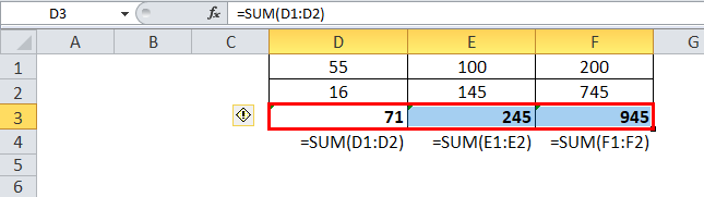
Now all the cells which you had selected got a formula hidden from the formula bar.

If you send this file to someone they will not be able to see the formula or edit it unless this worksheet is unprotected.
How Do I Find Hidden Formulas?
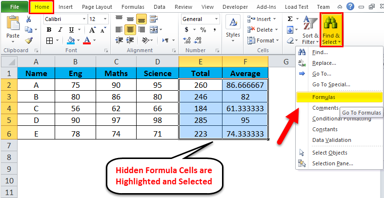
Once you protect a file using the above steps even you can’t see the formula until you unprotect the worksheet. But if you just want to find them from a protected worksheet where they are, you can use the “Go To Special” option.
- Go to Home Tab -> Editing -> Find & Select -> Go to Special.
- Select the “Formulas” option and it all four sub-option (Numbers, Text, Logical, Errors) and click OK.
- Once you click OK, Excel will select all the cells from the worksheet where you have formulas.
Hide a Formula without Protecting a Worksheet: I’m sure you have this thought in your mind how can I hide a formula without protecting a worksheet? I’m afraid there is no other method for this. You need to go this way. The only possible thing which I know is to create a macro code that runs at the opening of the workbook and hides the formula bar. But, again this is not a permanent solution.
Conclusion
This option not only helps you to hide formulas but also helps if you have any crucial calculations which you want to hide from others.
Until someone has the password, formulas are hidden and safe. I hope this tip will help you to manage your worksheets.
Have you ever tried to hide a formula before? Please share your views with me in the comment section, I’d love to hear from you.
And, make sure to share this tip with your friends.
При работе с таблицами Excel, наверняка, многие пользователи могли заметить, что если в какой-то ячейке содержится формула, то в специальной строке формул (справа от кнопки “fx”) мы увидим именно ее.

Довольно часто возникает необходимость в скрытии формул на листе. Это может быть связано с тем, что пользователь, например, не желает показывать их посторонним лицам. Давайте рассмотрим, каким образом это можно сделать в Эксель.
Метод 1. Включаем защиту листа
Результатом реализации данного метода является скрытие содержимого ячеек в строке формул и запрет на их редактирование, что в полной мере соответствует поставленной задаче.
- Для начала нужно выделить ячейки, содержимое которых мы хотим спрятать. Затем правой кнопкой мыши щелкаем по выделенному диапазону и раскрывшемся контекстном меню останавливаемся на строке “Формат ячеек”. Также вместо использования меню можно нажать комбинацию клавиш Ctrl+1 (после того, как нужная область ячеек была выделена).

- Переключаемся во вкладку “Защита” в открывшемся окне форматирования. Здесь ставим галочку напротив опции “Скрыть формулы”. Если в наши цели не входит защита ячеек от изменений, соответствующую галочку можно убрать. Однако, в большинстве случаев, данная функция важнее, чем само скрытие формул, поэтому, в нашем случаем мы тоже ее оставим. По готовности щелкаем OK.

- Теперь в основном окне программы переключаемся во вкладку “Рецензирование”, где в группе инструментов “Защита” выбираем функцию “Защитить лист”.

- В отобразившемся окошке оставляем стандартные настройки, вводим пароль (потребуется в дальнейшем для снятия защиты листа) и жмем OK.

- В окне подтверждения, которе появится следом, снова вводим ранее заданный пароль и жмем OK.

- В результате нам удалось скрыть формулы. Теперь при выборе защищенных ячеек в строке формул будет пусто.


Примечание: После активации защиты листа при попытке внести любые изменения в защищенные ячейки, программа будет выдавать соответствующее информационное сообщение.

При этом если мы для каких-то ячеек хотим оставить возможность редактирования (и выделения – для метода 2, о котором пойдет речь ниже), отметив их и перейдя в окно форматирования, снимаем галочку “Защищаемая ячейка”.

Например, в нашем случае мы можем скрыть формулу, но при этом оставить возможность менять количество по каждому наименованию и его стоимость. После того, как мы применим защиту листа, содержимое данных ячеек по-прежнему можно будет корректировать.

Метод 2. Запрещаем выделение ячеек
Данный метод не так часто используется по сравнению с рассмотренным выше. Наряду со скрытием информации в строке формул и запретом на редактирование защищенных ячеек, он также предполагает запрет на их выделение.
- Выделяем требуемый диапазон ячеек, в отношении которых хотим выполнить запланированные действия.
- Идем в окно форматирования и во вкладке “Защита” проверяем, стоит ли галочка напротив опции “Защищаемая ячейка” (должна быть включена по умолчанию). Если нет, ставим ее и щелкаем OK.
- Во вкладке “Рецензирование” щелкаем по кнопке “Защитить лист”.
- Откроется уже знакомое окошко для выбора параметров защиты и ввода пароля. Убираем галочку напротив опции “выделение заблокированных ячеек”, задаем пароль и щелкаем OK.
- Подтверждаем пароль, повторно набрав его, после чего жмем OK.
- В результате выполненных действий у нас больше не будет возможности не только просматривать содержимое ячеек в строке формул, но и выделять их.


Заключение
Таким образом, скрыть формулы в таблице Эксель можно двумя методами. Первый предполагает защиту ячеек с формулами от редактирования и скрытие их содержимого в строке формул. Второй – более строгий, в дополнение к результату, полученному с помощью первого метода, накладывает запрет, в т.ч., на выделение защищенных ячеек.
Excel Hide Formulas (Table of Contents)
- Introduction to Hide Formula in Excel
- Different ways to Hide the Formula in Excel
- #1 – To protect the worksheet and activate the hide formula option
- #2 – To hide the formula bar of an Excel workbook
Introduction to Hide Formula in Excel
There are two ways to Hide any formulas in Excel. The first way we can protect the current worksheet or workbook from Protect Sheet and Protect Workbook option, which is available in the Review menu option under the Changes section. There we need to provide the password to lock the changes in Sheet. This will prevent other people from changing their formulas. And other is by Format Cells option, which can be accessed by short cut key Ctrl + 1. From the Format Cells box, under the Protection tab, select the Hidden option and locked option. By doing this, it will lock the selected cell preventing it from editing.
- This feature in excel is introduced in order to hide the formulas from others.
- When we write a formula in an active cell, the formula is automatically displayed in the formula bar.

- Sometimes, it is needed to hide the formula for security or confidentiality reasons. In that case, we use the excel hide formula.
- Excel makes it simple to hide formulas from getting changed.
Example:
Different ways to Hide the Formula in Excel
There are different ways of hiding excel formulas to protect accidental or intentional changes in the worksheet, as mentioned below –
You can download this Hide Formula Excel Template here – Hide Formula Excel Template
- To protect the worksheet and activate the hide formula option.
- To hide the formula bar of the workbook.
#1 – To protect the worksheet and activate the hide formula option.
Steps to hide the Excel formula
Step 1: To Unprotect the Sheet
- The first step is to make sure that the worksheet is unprotected.
- To check the same, go to the Review tab in the Excel ribbon.
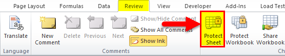
- If you find the Protect Sheet button in the toolbar, then it means the worksheet is not protected. In that case, you can directly start the steps to hide the formula from here on.
- If you find the Unprotect Sheet button in the toolbar, then it means the worksheet is protected. Click on the same and make the sheet unprotected by typing the correct password.
Step 2: To hide the Formula in Excel.
- As per the in-built feature of MS Excel, by default, the formula of the active cell appears in the formula bar.
- To hide the excel formula, select the range of cells for which the formula is needed to be hidden.
- Right-click the cell or range of cells. Select Format Cells or press Ctrl+1.
- Once the Format Cells dialog box appears, click on Protection.
- The locked check box is selected by default. The hidden checkbox is deselected by default. The selected Locked check box prevents the user from changing the contents of the cells in a sheet, whereas the Hidden checkbox is an optional feature. It needs to be selected manually. It helps in hiding the formula and prevents the user from seeing the same.
Step 3: To Protect the Sheet
- This step is very important in hiding the formula. The above formula will remain ineffective until the sheet is being protected.
- Go to the Review tab in the excel ribbon. Click on Protect Sheet.

- Protect Sheet dialog box will appear. Type the password to protect the sheet. Once the sheet is protected, no one except the real user can unprotect the sheet and make changes in it and then click OK.
Note: By default, Protect worksheet and contents of the locked cells check box is selected. Also, Select locked cells and Select unlocked cells checkboxes to remain selected by default.
- Confirm Password dialog box will appear. Retype the password, which will help to prevent a typographical error in the password from locking the spreadsheet forever. Click OK.
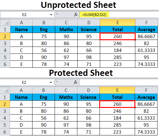
- Once the sheet is protected, the formula of the active cell will not be shown up in the formula bar. Thus the formulas in the cells are protected. Therefore, neither it can be seen or edited.
- Whenever you want to make changes to the protected sheet, the following message will be displayed.
Note: The user without a password can click on the cells but cannot make changes in the content of the protected sheet. To make the changes, first, make the protected sheet is unprotected.
How to Unprotect the Protected sheet?
- Select Review tab in excel ribbon. Click on Unprotect Sheet option.
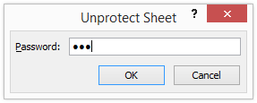
- Unprotect sheet dialog box will appear. Type in the password and then click Ok. The sheet will become unprotected.
#2 – To hide the formula bar of an Excel workbook
Formula bar exists below the formatting toolbar or ribbon area. It is divided into two different parts:-
The left part is the Name box where the active cell number is displayed.
On the right, the Formula of the active cell is displayed.
Steps to hide the formula bar:
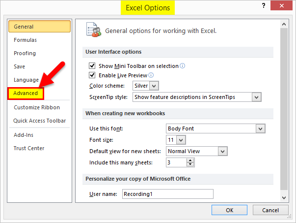
- Go to the File tab in the Excel ribbon. Select Options.
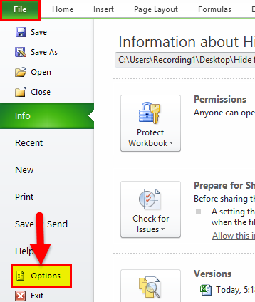
- Excel Options dialog box will appear. Select Advanced.
- On the right-hand side panel, scroll down to the Display section.
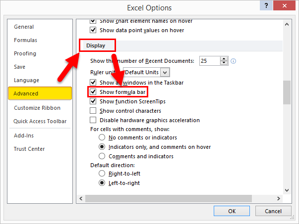
- Unselect the Show formula bar checkbox and then click OK.
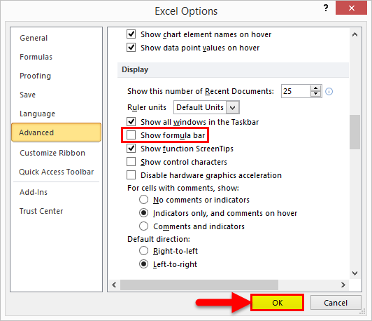
Note: If show formula bar check box is selected, the formula bar will be displayed; otherwise, it will not be displayed.
How can the Hidden formulas be found?
- Go to the Home tab in the Excel ribbon in the Editing section, select Find & Select and then click on the Formulas option.
- Excel will highlight and select all the cells that have formulas.
Things to Remember about the Hide Formula in Excel
- This option helps you hide the crucial and confidential formulas from others, thus protecting your documents.
- As discussed above, there are two ways of hiding formulas. In the first method, we can hide and protect the formulas sheet wise. In other words, in the same workbook, we can apply it to protect and hide the excel formula in one sheet, whereas the second sheet remains unprotected.
- In the protected worksheet, we can only see the data and put the cursor on the cells but cannot view the formulas and make changes in them.
- The second way to hide the formula bar applies across any file opened in the MS Excel application. The worksheets are not protected however formulas remain hidden because of the aforementioned feature.
Recommended Articles
This has been a guide to Hide Formula in Excel. Here we discuss how to use Hide Formula in Excel along with practical examples and a downloadable excel template. You can also go through our other suggested articles-
- Unhide Columns in Excel
- TRIM Formula in Excel
- Excel Show Formula
- Write Formula in Excel
Содержание
- How to Lock Formula Cells & Hide Formulas in Excel
- Notes on Cell Locking and Hiding
- Lock Formula Cells In Excel
- Step 1 – Unlock all the Cells in the Worksheet
- Step 2 – Lock the Cells in the Worksheet Containing the Formulas
- Step 3 – Protect the Worksheet
- Hide Formulas In Excel
- VBA to Lock and Hide Formulas In Excel
- Subscribe and be a part of our 15,000+ member family!
How to Lock Formula Cells & Hide Formulas in Excel
The need for locking cells comes with the ease of editing in Excel. Think of a calculation that has multiple columns referenced within the formula (e.g. net salary using taxes, allowances, and bonus calculations). If accidentally one value is changed, it affects the whole string of calculations and consequently the final amount (not to mention employee morale).
Such things can easily make your spreadsheets a scary thing. However, thankfully we have the option of locking the cells containing formulas to avoid intentional and unintentional tampering and editing; that’s what we will address today.
Locked cells cannot be edited, but it does not restrict us from seeing the formulas in the Formula Bar. While this isn’t a problem in most cases, but if you don’t want the formulas to be visible, you need to make them hidden. This tutorial will take you through locking formula cells and hiding formulas in Excel.

Table of Contents
Notes on Cell Locking and Hiding
This may come as a surprise but all cells are locked by default in Excel. The locked cells however are only truly locked from editing once the worksheet is protected.
Hidden cells also need sheet protection to hide the contents of the cells. This means that both cell locking and hiding need sheet protection to work.
To lock certain cells on a worksheet, all cells must be unlocked first. Then the specific cells can be selected and locked. Next, the sheet has to be protected to lock the cells from being changed.
Lock Formula Cells In Excel
Locking formula cells means that we will be locking some chosen cells. For that, we need to change the default setting of all the cells in the sheet (which is locked) to unlocked. Then we will select the formula cells and lock them. After locking the cells, the worksheet needs to be protected to lock the cells from being edited.
There is a nifty trick to automatically select all the formula cells in a sheet instead of selecting them manually. That nifty trick is to use Go To Special. We will use this feature to select the formula cells in the sheet to lock them.
Below are the steps to unlock all the cells, lock the formula cells and protect the worksheet. Let’s break them down, one by one.
Step 1 – Unlock all the Cells in the Worksheet
- Select all the cells in the worksheet (Ctrl + A).
- Launch the Format Cells dialog box by right-clicking any cell and selecting Format Cells from the right-click context menu (or using the keyboard shortcut Ctrl + 1).

- In the dialog box, go to the Protection The Locked checkbox will be ticked. Uncheck the Locked checkbox.

Now all the cells on the sheet are unlocked. This will not have any visual impact on the sheet unless the data contains formulas. In that case, you will see a green arrow in the top left corner of all formula cells. Selecting any of these cells will show the Trace Error button which will report exposed formulas due to unlocked cells.

Don’t worry locking these cells will fix this error and that is our next step.
Step 2 – Lock the Cells in the Worksheet Containing the Formulas
Now we will lock only the formula cells in the worksheet so that after the sheet is protected, only the formula cells cannot be changed. Instead of selecting the formula cells manually, we will use the Go To Special feature. Below are the steps to lock the formula cells in the worksheet with Go To Special:
- Select all the cells in the worksheet (Ctrl + A).
- In the Home tab, from the Editing section, click on the Find & Select From the drop-down list, select Go To Special to open the Go To Special dialog box.

- Select the Formulas radio button and make sure all the checkboxes under Formulas are checked. Then click OK.

As you can see below, all cells containing formulas on the worksheet will be selected.

The next step is to lock the selected formula cells.
- Launch the Format Cells dialog box by clicking on the dialog launcher (small arrow on the bottom right) in the Alignment section (or use the keyboard shortcut Ctrl + 1).
- In the Protection tab, check the Locked Then click OK.

Now that the formula cells are locked, the formula errors have disappeared.

To completely restrict the editing of locked cells, the worksheet needs to be protected, which is the next step.
Step 3 – Protect the Worksheet
To activate the properties of a locked cell, you have to protect the worksheet and the simple steps for doing that are as follows:
- Go to the Review From the Protect section, select the Protect Sheet command button.

- Confirm that the Protect worksheet and contents of locked cells checkbox is checked.

- In this Protect Sheet dialog window, you have the option of adding a password to unprotect the sheet. It can be helpful to keep a password to allow some users to edit the locked cells by sharing the password with them.
- Other controls of the worksheet are in Allow all users of this worksheet to: field. We are going with the default settings (top 2 checkboxes checked).
- After making the changes as you like, click OK.
Following these steps have protected the worksheet and locked the formula cells, disallowing any editing. Any cell other than the formula cells can be edited. Should you try to edit a cell containing a formula, a prompt will pop up notifying that the cell belongs to a protected sheet.

If a password had been set up in the Protect Sheet window, the user will be asked to enter the password while unprotecting the sheet from the Unprotect Sheet command button in the Review tab. With no password, the sheet can be unprotected by clicking the Unprotect Sheet command button straight away.

Hide Formulas In Excel
By hiding formulas, the formula of the cell will not display in the Formula Bar when the cell is selected. The process of hiding formulas is very similar to that of locking cells (with just an extra setting enabled). Like locked cells, hidden cells also work only once the sheet is protected.
The formula cells have to be selected to be hidden. We will use the Go To Special feature to select the formula cells to hide them. Here are the steps to select and hide the formula cells and to protect the sheet:
- Select all the cells in the worksheet (Ctrl + A).
- In the Home tab, from the Editing section, click on the Find & Select From the drop-down list, select Go To Special to open the Go To Special dialog box.
- Select the Formulas radio button and make sure all the checkboxes under Formulas are checked. Then click OK.
- All cells containing formulas on the worksheet will be selected like so:
The next step is to hide the selected formula cells.
- Launch the Format Cells dialog box by clicking on the dialog launcher (small arrow on the bottom right) in the Alignment section (or use the keyboard shortcut Ctrl + 1).
- In the Protection tab, check the Hidden Then click OK.

This has no visual impact on the sheet yet as the hidden properties only work once the sheet is protected. If you select any of the hidden cells right now, you can still see the formula in the formula bar. Let’s move on to protecting the sheet:
- Go to the Review From the Protect section, select the Protect Sheet command button.
- Confirm that the Protect worksheet and contents of locked cells checkbox is checked.
- In this Protect Sheet dialog window, you have the option of adding a password to unprotect the sheet. It can be helpful to keep a password to allow some users to edit the locked cells or view the formulas by sharing the password with them.
- Other controls of the worksheet are in the Allow all users of this worksheet to: field. We are going with the default settings (top 2 checkboxes checked).
- After making the changes as you like, click OK.
Following these steps have protected the worksheet and hidden the formula cells. If you select any cell containing a formula now, you can see that the Formula Bar will not display its formula.

If you had set up a password in the Protect Sheet window, the user will be asked to enter the password while unprotecting the sheet from the Unprotect Sheet command button in the Review tab. With no password, the sheet can be unprotected by clicking the Unprotect Sheet command button.
VBA to Lock and Hide Formulas In Excel
You can ditch all the steps above and select, lock and hide formulas and protect the worksheet using VBA. All you have to do is access the VBA editor, feed in the right code, run the command and that’s job done!
VBA (Visual Basic for Applications) is a programming tool for MS Office applications. We can use codes in VBA to get various tasks done in Excel, especially if they are laborious or repetitive.
Below we will show you how to use VBA to lock and hide formulas and protect the sheet, all using one code. The steps are:
- Press Alt + F11 to run the VBA editor. If you don’t have the Developer tab, you can add it by customizing the ribbon and then access the VBA editor using the Visual Basic button.
- Click on the Insert tab and select Module from the list.

- In the opened module window, copy and paste the following code:

- Close the module window and the VBA editor.
- Go to the View tab and select the Macros command button.

- Select the relevant macro and then select Run.

Using the above-mentioned code, we have locked and hidden the formula cells and protected the sheet. If you try editing a formula cell, you will receive a prompt, disabling you from editing. That confirms the formula cells are locked.
Selecting any formula cell, you can see below that the formula is not visible in the Formula Bar. This confirms the formula cells are hidden.

Both the locked and hidden properties are working which means the sheet is protected which is also confirmed from the Review tab.
Now let’s lock that up and stop right here. We hope we gave you the full particulars on protecting the formula cells from all sorts of tweaking. We’ll be back, unlocking and unraveling more Excel mysteries; be ready to keep up!
Subscribe and be a part of our 15,000+ member family!
Now subscribe to Excel Trick and get a free copy of our ebook «200+ Excel Shortcuts» (printable format) to catapult your productivity.
Источник
Home > Microsoft Excel > How to Hide Formulas in Excel? 2 Different Approaches
(Note: This guide on how to hide formulas in Excel is suitable for all Excel versions including Office 365)
Excel deals with large amounts of data in which the values operate using a variety of functions and formulas. When you enter a formula in Excel, the formula that pertains to the cell always shows up on the formula bar.
This might be a great way to know what formula is used to obtain the particular value. But in some cases, the appearance of formulas might be a little irrelevant. So, what do you do when you don’t want the formula to appear in the formula bar in Excel?
In this article, I will show you how to hide formulas in Excel using 2 different approaches, without hiding the formula bar completely.
You’ll Learn:
- Why Hide Formulas in Excel?
- How to Hide Formulas in Excel?
- Hide the Worksheet by Making the Cells Non-Editable
- Hide Only the Cells with Formulas and Make Other Cells Editable

Watch this Video on How to Hide Formulas in Excel
Related Reads:
How to Calculate Percentile in Excel? 3 Useful Formulas
The FORMULATEXT Excel Function – 2 Best Examples
How to Round Up in Excel(and Round Down)?
Why Hide Formulas in Excel?
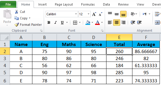
Before we learn how to hide formulas in Excel, let us see how a formula shows up in Excel and why we need to hide them with an example.
When you enter a formula in any cell, they show up in the formula bar above the column. The value which populates the cell is a result of the formula or function consisting of variables, other cells, and operands.

Though the formula may be a great way to understand how we have obtained the value, in some cases, they do feel a bit irrelevant.
Consider that you have to share the Excel sheet with a group of unrelated people. In such cases, it is better to keep the formulas and functions hidden, thereby maintaining confidentiality. Also, this helps in protecting the file from being edited and the user will be able to only view the data.
In addition, consider the above example where the formula =RAND() is used to find the random value. When showing it as an example or while taking a screenshot, the presence of the formula cell might not be necessary.
In such cases, it would be better to hide only the formula without hiding the formula bar.
How to Hide Formulas in Excel?
Hide the Worksheet by Making the Cells Non-Editable
This is one method to hide the formula showing up in the formula bar. However, using this method to hide the formula bar also protects the sheet and makes the cell uneditable.
To hide the formulas and to make the cells uneditable, first, select the cells from which you don’t want the formula to show up. You can select a single cell, an adjacent group of cells, non-adjacent cells, and even the whole sheet.

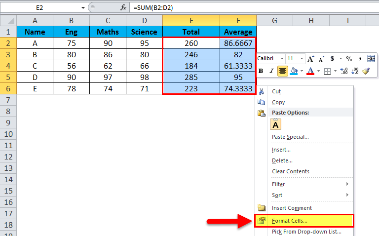
After selecting the cells, right-click on the selected cells and click on Format Cells.

Another way to arrive at the Format Cells dialog box is by navigating to Home. Under the Number section, click on Number Format which appears as a small dropdown arrow.

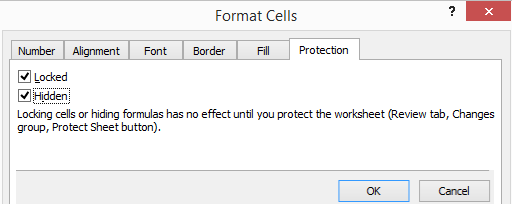
This opens up a Format Cells dialog box. Go to the Protection tab and check the checkbox for Hidden. Click OK.

Once you have hidden the cells, navigate to Review. Under the Protect section, click on Protect Sheet.

Once you click on the Protect sheet, a dialog box appears. If the sheet is confidential to you, enter a password. You can unprotect the sheet only by using this password. In this case, let us leave the password textbox blank.
Make sure the checkbox for Protect worksheet and contents of locked cells is checked. The below two checkboxes for select locked cells and select unlocked cells are checked. This only lets the user click on them, but they are detained from doing any operation on the cells. Click OK.

This hides the formulas from showing up on the formula bar. When you click on any of the cells, you cannot see the formulas. In this case, when I previously clicked on the cells the formula =RAND() showed up in the formula bar. Now, after protecting the sheet the formulas are hidden for the selected cells.

In addition to hiding the formulas, this method also protects the sheet from being edited or altered.
Suggested Reads:
How to Use the PROPER Function in Excel? 3 Easy Examples
Excel DATEVALUE – A Step-by-Step Guide
How to Use SUMPRODUCT Function in Excel? 5 Easy Examples
Hide Only the Cells with Formulas and Make Other Cells Editable
In the above method, we saw how to hide the formulas from showing up in the formula bar when a cell is selected, making the selected cells uneditable.
However, in some cases, the user might have to input some data. For example, any data entry sheet to be circulated should be editable by other users. Then the method of protecting the entire worksheet by making them uneditable won’t be useful this time.
So, you can use the below-mentioned method to only hide the cells with formulas and keep the rest of the cells editable. This method is especially useful when there is a large amount of data and you cannot identify where the formulas are and which cells to hide or unhide.
Consider an example where the sheet contains the profit and losses made by salesmen and the clients will rate them. Here, some cells require editing when different clients rate a salesman.
To make this method work, let us first disable the lock property of all the cells in the sheet.
Select the entire sheet either by clicking on the gray arrow on the top-left corner of the column or by using the keyboard shortcut Ctrl + A.

Now to unlock the cell, navigate to Home. Under Number, click on Number Format which opens a dialog box.
Under the Protection tab, uncheck the checkbox for Locked. And, click OK.

This disables the lock property of the cells and makes them editable. Once the cells are unlocked, the cell containing the formulas throws up a warning message.

Now then, let us see how to protect only the cells which have formulas.
Again select all the cells in the sheet by using the gray triangle on the top-left of the sheet or by pressing Ctrl+A.
After you have selected the whole sheet, we only need to identify the cells which only have the formulas. To do that, navigate to Home. Click on the dropdown from Find & Select and click on Go To Special.

This opens up the Go To Special dialog box. In the dialog box, select Formulas and make sure all the checkboxes under the Formulas header are checked. Click OK. This step helps Excel identify the cells with formulas and selects them.

After the formulas are selected, let us now lock and hide the cells. You can either navigate to Home and click on Number and Number Format, or right-click on the selected cells and click on Format Cells. You can also use the keyboard shortcut key Ctrl+1.
In the Format Cells dialog box, under Protection, check the checkboxes for both Locked and Hidden. Click OK.

Now, you can see the warning symbols disappear on the cells with formulas.
After this, navigate to Review. Under the Protect section, click on Protect Sheet. Enter the password to protect the sheet and check the checkboxes for Protect worksheet and content for locked cells. Select the locked and unlocked cells, and click OK.

This locks only the cells with formulas, whereas the rest of the cells remain editable. If you click on any of the cells containing the formula, the formula does not appear on the formula bar, and also you cannot alter them. Whereas you can edit any of the other cells which do not contain a formula.

Also Read:
How to Fix the #Div/0 Error in Excel? 2 Easy Methods
How to Use ISTEXT in Excel? With 3 Different Methods
Short Date Format in Excel – 3 Different Methods
FAQs
Is there any way to hide without protecting the sheet?
No, there is no way to hide formulas in Excel without protecting the sheet. However, you can use VBA codes, but they can sometimes be inconsistent and lead to other errors.
What to do when you lose the password for a protected file?
There is no way in Excel to get back the password and unprotect the sheet using conventional methods. However, there are a lot of hacks and workarounds on the internet which might help you unprotect the sheet.
How can you remove only formulas and keep values in Excel?
You can copy the cells which contain the values, then paste them onto another sheet (or in a different place on the same sheet) by pasting them as Values.
Closing Thoughts
In this article, we saw how to hide formulas in Excel without hiding the formula bar. You can either hide the formulas by making the whole sheet protected and non-editable, or you can just pinpoint and protect the cells containing the formulas by keeping the other cells editable. Both are useful in their ways, you can use the method which suits your purpose better.
Please visit our free resources center to know more about the date and time functions.
We have high-quality Excel guides and you will be really excited to know how handy and useful these functions are.
Simon Sez IT has been teaching Excel for over ten years. For a low monthly fee, you can access 130+ IT training courses. Click here for advanced Excel courses with in-depth training modules.
Simon Calder

Chris “Simon” Calder was working as a Project Manager in IT for one of Los Angeles’ most prestigious cultural institutions, LACMA.He taught himself to use Microsoft Project from a giant textbook and hated every moment of it. Online learning was in its infancy then, but he spotted an opportunity and made an online MS Project course — the rest, as they say, is history!