Help with functions in excel - Word и Excel - помощь в работе с программами

Function	Description
AVEDEV function	Returns the average of the absolute deviations of data points from their mean
AVERAGE function	Returns the average of its arguments
AVERAGEA function	Returns the average of its arguments, including numbers, text, and logical values
AVERAGEIF function	Returns the average (arithmetic mean) of all the cells in a range that meet a given criteria
AVERAGEIFS function	Returns the average (arithmetic mean) of all cells that meet multiple criteria
BETA.DIST function	Returns the beta cumulative distribution function
BETA.INV function	Returns the inverse of the cumulative distribution function for a specified beta distribution
BINOM.DIST function	Returns the individual term binomial distribution probability
BINOM.DIST.RANGE function	Returns the probability of a trial result using a binomial distribution
BINOM.INV function	Returns the smallest value for which the cumulative binomial distribution is less than or equal to a criterion value
CHISQ.DIST function	Returns the cumulative beta probability density function
CHISQ.DIST.RT function	Returns the one-tailed probability of the chi-squared distribution
CHISQ.INV function	Returns the cumulative beta probability density function
CHISQ.INV.RT function	Returns the inverse of the one-tailed probability of the chi-squared distribution
CHISQ.TEST function	Returns the test for independence
CONFIDENCE.NORM function	Returns the confidence interval for a population mean
CONFIDENCE.T function	Returns the confidence interval for a population mean, using a Student’s t distribution
CORREL function	Returns the correlation coefficient between two data sets
COUNT function	Counts how many numbers are in the list of arguments
COUNTA function	Counts how many values are in the list of arguments
COUNTBLANK function	Counts the number of blank cells within a range
COUNTIF function	Counts the number of cells within a range that meet the given criteria
COUNTIFS function	Counts the number of cells within a range that meet multiple criteria
COVARIANCE.P function	Returns covariance, the average of the products of paired deviations
COVARIANCE.S function	Returns the sample covariance, the average of the products deviations for each data point pair in two data sets
DEVSQ function	Returns the sum of squares of deviations
EXPON.DIST function	Returns the exponential distribution
F.DIST function	Returns the F probability distribution
F.DIST.RT function	Returns the F probability distribution
F.INV function	Returns the inverse of the F probability distribution
F.INV.RT function	Returns the inverse of the F probability distribution
F.TEST function	Returns the result of an F-test
FISHER function	Returns the Fisher transformation
FISHERINV function	Returns the inverse of the Fisher transformation
FORECAST function	Returns a value along a linear trend Note: In Excel 2016, this function is replaced with FORECAST.LINEAR as part of the new Forecasting functions, but it’s still available for compatibility with earlier versions.
FORECAST.ETS function	Returns a future value based on existing (historical) values by using the AAA version of the Exponential Smoothing (ETS) algorithm
FORECAST.ETS.CONFINT function	Returns a confidence interval for the forecast value at the specified target date
FORECAST.ETS.SEASONALITY function	Returns the length of the repetitive pattern Excel detects for the specified time series
FORECAST.ETS.STAT function	Returns a statistical value as a result of time series forecasting
FORECAST.LINEAR function	Returns a future value based on existing values
FREQUENCY function	Returns a frequency distribution as a vertical array
GAMMA function	Returns the Gamma function value
GAMMA.DIST function	Returns the gamma distribution
GAMMA.INV function	Returns the inverse of the gamma cumulative distribution
GAMMALN function	Returns the natural logarithm of the gamma function, Γ(x)
GAMMALN.PRECISE function	Returns the natural logarithm of the gamma function, Γ(x)
GAUSS function	Returns 0.5 less than the standard normal cumulative distribution
GEOMEAN function	Returns the geometric mean
GROWTH function	Returns values along an exponential trend
HARMEAN function	Returns the harmonic mean
HYPGEOM.DIST function	Returns the hypergeometric distribution
INTERCEPT function	Returns the intercept of the linear regression line
KURT function	Returns the kurtosis of a data set
LARGE function	Returns the k-th largest value in a data set
LINEST function	Returns the parameters of a linear trend
LOGEST function	Returns the parameters of an exponential trend
LOGNORM.DIST function	Returns the cumulative lognormal distribution
LOGNORM.INV function	Returns the inverse of the lognormal cumulative distribution
MAX function	Returns the maximum value in a list of arguments
MAXA function	Returns the maximum value in a list of arguments, including numbers, text, and logical values
MAXIFS function	Returns the maximum value among cells specified by a given set of conditions or criteria
MEDIAN function	Returns the median of the given numbers
MIN function	Returns the minimum value in a list of arguments
MINA function	Returns the smallest value in a list of arguments, including numbers, text, and logical values
MINIFS function	Returns the minimum value among cells specified by a given set of conditions or criteria.
MODE.MULT function	Returns a vertical array of the most frequently occurring, or repetitive values in an array or range of data
MODE.SNGL function	Returns the most common value in a data set
NEGBINOM.DIST function	Returns the negative binomial distribution
NORM.DIST function	Returns the normal cumulative distribution
NORM.INV function	Returns the inverse of the normal cumulative distribution
NORM.S.DIST function	Returns the standard normal cumulative distribution
NORM.S.INV function	Returns the inverse of the standard normal cumulative distribution
PEARSON function	Returns the Pearson product moment correlation coefficient
PERCENTILE.EXC function	Returns the k-th percentile of values in a range, where k is in the range 0..1, exclusive
PERCENTILE.INC function	Returns the k-th percentile of values in a range
PERCENTRANK.EXC function	Returns the rank of a value in a data set as a percentage (0..1, exclusive) of the data set
PERCENTRANK.INC function	Returns the percentage rank of a value in a data set
PERMUT function	Returns the number of permutations for a given number of objects
PERMUTATIONA function	Returns the number of permutations for a given number of objects (with repetitions) that can be selected from the total objects
PHI function	Returns the value of the density function for a standard normal distribution
POISSON.DIST function	Returns the Poisson distribution
PROB function	Returns the probability that values in a range are between two limits
QUARTILE.EXC function	Returns the quartile of the data set, based on percentile values from 0..1, exclusive
QUARTILE.INC function	Returns the quartile of a data set
RANK.AVG function	Returns the rank of a number in a list of numbers
RANK.EQ function	Returns the rank of a number in a list of numbers
RSQ function	Returns the square of the Pearson product moment correlation coefficient
SKEW function	Returns the skewness of a distribution
SKEW.P function	Returns the skewness of a distribution based on a population: a characterization of the degree of asymmetry of a distribution around its mean
SLOPE function	Returns the slope of the linear regression line
SMALL function	Returns the k-th smallest value in a data set
STANDARDIZE function	Returns a normalized value
STDEV.P function	Calculates standard deviation based on the entire population
STDEV.S function	Estimates standard deviation based on a sample
STDEVA function	Estimates standard deviation based on a sample, including numbers, text, and logical values
STDEVPA function	Calculates standard deviation based on the entire population, including numbers, text, and logical values
STEYX function	Returns the standard error of the predicted y-value for each x in the regression
T.DIST function	Returns the Percentage Points (probability) for the Student t-distribution
T.DIST.2T function	Returns the Percentage Points (probability) for the Student t-distribution
T.DIST.RT function	Returns the Student’s t-distribution
T.INV function	Returns the t-value of the Student’s t-distribution as a function of the probability and the degrees of freedom
T.INV.2T function	Returns the inverse of the Student’s t-distribution
T.TEST function	Returns the probability associated with a Student’s t-test
TREND function	Returns values along a linear trend
TRIMMEAN function	Returns the mean of the interior of a data set
VAR.P function	Calculates variance based on the entire population
VAR.S function	Estimates variance based on a sample
VARA function	Estimates variance based on a sample, including numbers, text, and logical values
VARPA function	Calculates variance based on the entire population, including numbers, text, and logical values
WEIBULL.DIST function	Returns the Weibull distribution
Z.TEST function	Returns the one-tailed probability-value of a z-test

Источник

Below is a brief overview of about 100 important Excel functions you should know, with links to detailed examples. We also have a large list of example formulas, a more complete list of Excel functions, and video training. If you are new to Excel formulas, see this introduction.

Note: Excel now includes Dynamic Array formulas, which offer important new functions.

Date and Time Functions

Excel provides many functions to work with dates and times.

NOW and TODAY

You can get the current date with the TODAY function and the current date and time with the NOW Function. Technically, the NOW function returns the current date and time, but you can format as time only, as seen below:

TODAY() // returns current date
NOW() // returns current time

Note: these are volatile functions and will recalculate with every worksheet change. If you want a static value, use date and time shortcuts.

DAY, MONTH, YEAR, and DATE

You can use the DAY, MONTH, and YEAR functions to disassemble any date into its raw components, and the DATE function to put things back together again.

=DAY("14-Nov-2018") // returns 14
=MONTH("14-Nov-2018") // returns 11
=YEAR("14-Nov-2018") // returns 2018
=DATE(2018,11,14) // returns 14-Nov-2018

HOUR, MINUTE, SECOND, and TIME

Excel provides a set of parallel functions for times. You can use the HOUR, MINUTE, and SECOND functions to extract pieces of a time, and you can assemble a TIME from individual components with the TIME function.

=HOUR("10:30") // returns 10
=MINUTE("10:30") // returns 30
=SECOND("10:30") // returns 0
=TIME(10,30,0) // returns 10:30

DATEDIF and YEARFRAC

You can use the DATEDIF function to get time between dates in years, months, or days. DATEDIF can also be configured to get total time in «normalized» denominations, i.e. «2 years and 6 months and 27 days».

Use YEARFRAC to get fractional years:

=YEARFRAC("14-Nov-2018","10-Jun-2021") // returns 2.57

EDATE and EOMONTH

A common task with dates is to shift a date forward (or backward) by a given number of months. You can use the EDATE and EOMONTH functions for this. EDATE moves by month and retains the day. EOMONTH works the same way, but always returns the last day of the month.

EDATE(date,6) // 6 months forward
EOMONTH(date,6) // 6 months forward (end of month)

WORKDAY and NETWORKDAYS

To figure out a date n working days in the future, you can use the WORKDAY function. To calculate the number of workdays between two dates, you can use NETWORKDAYS.

WORKDAY(start,n,holidays) // date n workdays in future

Video: How to calculate due dates with WORKDAY

NETWORKDAYS(start,end,holidays) // number of workdays between dates

Note: Both functions automatically skip weekends (Saturday and Sunday) and will also skip holidays, if provided. If you need more flexibility on what days are considered weekends, see the WORKDAY.INTL function and NETWORKDAYS.INTL function.

WEEKDAY and WEEKNUM

To figure out the day of week from a date, Excel provides the WEEKDAY function. WEEKDAY returns a number between 1-7 that indicates Sunday, Monday, Tuesday, etc. Use the WEEKNUM function to get the week number in a given year.

=WEEKDAY(date) // returns a number 1-7
=WEEKNUM(date) // returns week number in year

Engineering

CONVERT

Most Engineering functions are pretty technical…you’ll find a lot of functions for complex numbers in this section. However, the CONVERT function is quite useful for everyday unit conversions. You can use CONVERT to change units for distance, weight, temperature, and much more.

=CONVERT(72,"F","C") // returns 22.2

Information Functions

ISBLANK, ISERROR, ISNUMBER, and ISFORMULA

Excel provides many functions for checking the value in a cell, including ISNUMBER, ISTEXT, ISLOGICAL, ISBLANK, ISERROR, and ISFORMULA These functions are sometimes called the «IS» functions, and they all return TRUE or FALSE based on a cell’s contents.

Excel also has ISODD and ISEVEN functions that will test a number to see if it’s even or odd.

By the way, the green fill in the screenshot above is applied automatically with a conditional formatting formula.

Logical Functions

Excel’s logical functions are a key building block of many advanced formulas. Logical functions return the boolean values TRUE or FALSE. If you need a primer on logical formulas, this video goes through many examples.

AND, OR and NOT

The core of Excel’s logical functions are the AND function, the OR function, and the NOT function. In the screen below, each of these function is used to run a simple test on the values in column B:

=AND(B5>3,B5<9)
=OR(B5=3,B5=9)
=NOT(B5=2)

Video: How to build logical formulas
Guide: 50 examples of formula criteria

IFERROR and IFNA

The IFERROR function and IFNA function can be used as a simple way to trap and handle errors. In the screen below, VLOOKUP is used to retrieve cost from a menu item. Column F contains just a VLOOKUP function, with no error handling. Column G shows how to use IFNA with VLOOKUP to display a custom message when an unrecognized item is entered.

=VLOOKUP(E5,menu,2,0) // no error trapping
=IFNA(VLOOKUP(E5,menu,2,0),"Not found") // catch errors

Whereas IFNA only catches an #N/A error, the IFERROR function will catch any formula error.

IF and IFS functions

The IF function is one of the most used functions in Excel. In the screen below, IF checks test scores and assigns «pass» or «fail»:

Multiple IF functions can be nested together to perform more complex logical tests.

New in Excel 2019 and Excel 365, the IFS function can run multiple logical tests without nesting IFs.

=IFS(C5<60,"F",C5<70,"D",C5<80,"C",C5<90,"B",C5>=90,"A")

Lookup and Reference Functions

VLOOKUP and HLOOKUP

Excel offers a number of functions to lookup and retrieve data. Most famous of all is VLOOKUP:

=VLOOKUP(C5,$F$5:$G$7,2,TRUE)

More: 23 things to know about VLOOKUP.

HLOOKUP works like VLOOKUP, but expects data arranged horizontally:

=HLOOKUP(C5,$G$4:$I$5,2,TRUE)

INDEX and MATCH

For more complicated lookups, INDEX and MATCH offers more flexibility and power:

=INDEX(C5:E12,MATCH(H4,B5:B12,0),MATCH(H5,C4:E4,0))

Both the INDEX function and the MATCH function are powerhouse functions that turn up in all kinds of formulas.

More: How to use INDEX and MATCH

LOOKUP

The LOOKUP function has default behaviors that make it useful when solving certain problems. LOOKUP assumes values are sorted in ascending order and always performs an approximate match. When LOOKUP can’t find a match, it will match the next smallest value. In the example below we are using LOOKUP to find the last entry in a column:

ROW and COLUMN

You can use the ROW function and COLUMN function to find row and column numbers on a worksheet. Notice both ROW and COLUMN return values for the current cell if no reference is supplied:

The row function also shows up often in advanced formulas that process data with relative row numbers.

ROWS and COLUMNS

The ROWS function and COLUMNS function provide a count of rows in a reference. In the screen below, we are counting rows and columns in an Excel Table named «Table1».

Note ROWS returns a count of data rows in a table, excluding the header row. By the way, here are 23 things to know about Excel Tables.

HYPERLINK

You can use the HYPERLINK function to construct a link with a formula. Note HYPERLINK lets you build both external links and internal links:

=HYPERLINK(C5,B5)

GETPIVOTDATA

The GETPIVOTDATA function is useful for retrieving information from existing pivot tables.

=GETPIVOTDATA("Sales",$B$4,"Region",I6,"Product",I7)

CHOOSE

The CHOOSE function is handy any time you need to make a choice based on a number:

=CHOOSE(2,"red","blue","green") // returns "blue"

Video: How to use the CHOOSE function

TRANSPOSE

The TRANSPOSE function gives you an easy way to transpose vertical data to horizontal, and vice versa.

{=TRANSPOSE(B4:C9)}

Note: TRANSPOSE is a formula and is, therefore, dynamic. If you just need to do a one-time transpose operation, use Paste Special instead.

OFFSET

The OFFSET function is useful for all kinds of dynamic ranges. From a starting location, it lets you specify row and column offsets, and also the final row and column size. The result is a range that can respond dynamically to changing conditions and inputs. You can feed this range to other functions, as in the screen below, where OFFSET builds a range that is fed to the SUM function:

=SUM(OFFSET(B4,1,I4,4,1)) // sum of Q3

INDIRECT

The INDIRECT function allows you to build references as text. This concept is a bit tricky to understand at first, but it can be useful in many situations. Below, we are using INDIRECT to get values from cell A1 in 5 different worksheets. Each reference is dynamic. If a sheet name changes, the reference will update.

=INDIRECT(B5&"!A1") // =Sheet1!A1

The INDIRECT function is also used to «lock» references so they won’t change, when rows or columns are added or deleted. For more details, see linked examples at the bottom of the INDIRECT function page.

Caution: both OFFSET and INDIRECT are volatile functions and can slow down large or complicated spreadsheets.

STATISTICAL Functions

COUNT and COUNTA

You can count numbers with the COUNT function and non-empty cells with COUNTA. You can count blank cells with COUNTBLANK, but in the screen below we are counting blank cells with COUNTIF, which is more generally useful.

=COUNT(B5:F5) // count numbers
=COUNTA(B5:F5) // count numbers and text
=COUNTIF(B5:F5,"") // count blanks

COUNTIF and COUNTIFS

For conditional counts, the COUNTIF function can apply one criteria. The COUNTIFS function can apply multiple criteria at the same time:

=COUNTIF(C5:C12,"red") // count red
=COUNTIF(F5:F12,">50") // count total > 50
=COUNTIFS(C5:C12,"red",D5:D12,"TX") // red and tx
=COUNTIFS(C5:C12,"blue",F5:F12,">50") // blue > 50

Video: How to use the COUNTIF function

SUM, SUMIF, SUMIFS

To sum everything, use the SUM function. To sum conditionally, use SUMIF or SUMIFS. Following the same pattern as the counting functions, the SUMIF function can apply only one criteria while the SUMIFS function can apply multiple criteria.

=SUM(F5:F12) // everything
=SUMIF(C5:C12,"red",F5:F12) // red only
=SUMIF(F5:F12,">50") // over 50
=SUMIFS(F5:F12,C5:C12,"red",D5:D12,"tx") // red & tx
=SUMIFS(F5:F12,C5:C12,"blue",F5:F12,">50") // blue & >50

Video: How to use the SUMIF function

AVERAGE, AVERAGEIF, and AVERAGEIFS

Following the same pattern, you can calculate an average with AVERAGE, AVERAGEIF, and AVERAGEIFS.

=AVERAGE(F5:F12) // all
=AVERAGEIF(C5:C12,"red",F5:F12) // red only
=AVERAGEIFS(F5:F12,C5:C12,"red",D5:D12,"tx") // red and tx

MIN, MAX, LARGE, SMALL

You can find largest and smallest values with MAX and MIN, and nth largest and smallest values with LARGE and SMALL. In the screen below, data is the named range C5:C13, used in all formulas.

=MAX(data) // largest
=MIN(data) // smallest
=LARGE(data,1) // 1st largest
=LARGE(data,2) // 2nd largest
=LARGE(data,3) // 3rd largest
=SMALL(data,1) // 1st smallest
=SMALL(data,2) // 2nd smallest
=SMALL(data,3) // 3rd smallest

Video: How to find the nth smallest or largest value

MINIFS, MAXIFS

The MINIFS and MAXIFS. These functions let you find minimum and maximum values with conditions:

=MAXIFS(D5:D15,C5:C15,"female") // highest female
=MAXIFS(D5:D15,C5:C15,"male") // highest male
=MINIFS(D5:D15,C5:C15,"female") // lowest female
=MINIFS(D5:D15,C5:C15,"male") // lowest male

Note: MINIFS and MAXIFS are new in Excel via Office 365 and Excel 2019.

MODE

The MODE function returns the most commonly occurring number in a range:

=MODE(B5:G5) // returns 1

RANK

To rank values largest to smallest, or smallest to largest, use the RANK function:

Video: How to rank values with the RANK function

MATH Functions

ABS

To change negative values to positive use the ABS function.

=ABS(-134.50) // returns 134.50

RAND and RANDBETWEEN

Both the RAND function and RANDBETWEEN function can generate random numbers on the fly. RAND creates long decimal numbers between zero and 1. RANDBETWEEN generates random integers between two given numbers.

=RAND() // between zero and 1
=RANDBETWEEN(1,100) // between 1 and 100

ROUND, ROUNDUP, ROUNDDOWN, INT

To round values up or down, use the ROUND function. To force rounding up to a given number of digits, use ROUNDUP. To force rounding down, use ROUNDDOWN. To discard the decimal part of a number altogether, use the INT function.

=ROUND(11.777,1) // returns 11.8
=ROUNDUP(11.777) // returns 11.8
=ROUNDDOWN(11.777,1) // returns 11.7
=INT(11.777) // returns 11

MROUND, CEILING, FLOOR

To round values to the nearest multiple use the MROUND function. The FLOOR function and CEILING function also round to a given multiple. FLOOR forces rounding down, and CEILING forces rounding up.

=MROUND(13.85,.25) // returns 13.75
=CEILING(13.85,.25) // returns 14
=FLOOR(13.85,.25) // returns 13.75

MOD

The MOD function returns the remainder after division. This sounds boring and geeky, but MOD turns up in all kinds of formulas, especially formulas that need to do something «every nth time». In the screen below, you can see how MOD returns zero every third number when the divisor is 3:

SUMPRODUCT

The SUMPRODUCT function is a powerful and versatile tool when dealing with all kinds of data. You can use SUMPRODUCT to easily count and sum based on criteria, and you can use it in elegant ways that just don’t work with COUNTIFS and SUMIFS. In the screen below, we are using SUMPRODUCT to count and sum orders in March. See the SUMPRODUCT page for details and links to many examples.

=SUMPRODUCT(--(MONTH(B5:B12)=3)) // count March
=SUMPRODUCT(--(MONTH(B5:B12)=3),C5:C12) // sum March

SUBTOTAL

The SUBTOTAL function is an «aggregate function» that can perform a number of operations on a set of data. All told, SUBTOTAL can perform 11 operations, including SUM, AVERAGE, COUNT, MAX, MIN, etc. (see this page for the full list). The key feature of SUBTOTAL is that it will ignore rows that have been «filtered out» of an Excel Table, and, optionally, rows that have been manually hidden. In the screen below, SUBTOTAL is used to count and sum only the 7 visible rows in the table:

=SUBTOTAL(3,B5:B14) // returns 7
=SUBTOTAL(9,F5:F14) // returns 9.54

AGGREGATE

Like SUBTOTAL, the AGGREGATE function can also run a number of aggregate operations on a set of data and can optionally ignore hidden rows. The key differences are that AGGREGATE can run more operations (19 total) and can also ignore errors.

In the screen below, AGGREGATE is used to perform MIN, MAX, LARGE and SMALL operations while ignoring errors. Normally, the error in cell B9 would prevent these functions from returning a result. See this page for a full list of operations AGGREGATE can perform.

=AGGREGATE(4,6,values) // MAX ignore errors, returns 100
=AGGREGATE(5,6,values) // MIN ignore errors, returns 75

TEXT Functions

LEFT, RIGHT, MID

To extract characters from the left, right, or middle of text, use LEFT, RIGHT, and MID functions:

=LEFT("ABC-1234-RED",3) // returns "ABC"
=MID("ABC-1234-RED",5,4) // returns "1234"
=RIGHT("ABC-1234-RED",3) // returns "RED"

LEN

The LEN function will return the length of a text string. LEN shows up in a lot of formulas that count words or characters.

FIND, SEARCH

To look for specific text in a cell, use the FIND function or SEARCH function. These functions return the numeric position of matching text, but SEARCH allows wildcards and FIND is case-sensitive. Both functions will throw an error when text is not found, so wrap in the ISNUMBER function to return TRUE or FALSE (example here).

=FIND("Better the devil you know","devil") // returns 12
=SEARCH("This is not my beautiful wife","bea*") // returns 12

REPLACE, SUBSTITUTE

To replace text by position, use the REPLACE function. To replace text by matching, use the SUBSTITUTE function. In the first example, REPLACE removes the two asterisks (**) by replacing the first two characters with an empty string («»). In the second example, SUBSTITUTE removes all hash characters (#) by replacing «#» with «».

=REPLACE("**Red",1,2,"") // returns "Red"
=SUBSTITUTE("##Red##","#","") // returns "Red"

CODE, CHAR

To figure out the numeric code for a character, use the CODE function. To translate the numeric code back to a character, use the CHAR function. In the example below, CODE translates each character in column B to its corresponding code. In column F, CHAR translates the code back to a character.

=CODE("a") // returns 97
=CHAR(97) // returns "a"

Video: How to use the CODE and CHAR functions

TRIM, CLEAN

To get rid of extra space in text, use the TRIM function. To remove line breaks and other non-printing characters, use CLEAN.

=TRIM(A1) // remove extra space
=CLEAN(A1) // remove line breaks

Video: How to clean text with TRIM and CLEAN

CONCAT, TEXTJOIN, CONCATENATE

New in Excel via Office 365 are CONCAT and TEXTJOIN. The CONCAT function lets you concatenate (join) multiple values, including a range of values without a delimiter. The TEXTJOIN function does the same thing, but allows you to specify a delimiter and can also ignore empty values.

=TEXTJOIN(",",TRUE,B4:H4) // returns "red,blue,green,pink,black"
=CONCAT(B7:H7) // returns "8675309"

Excel also provides the CONCATENATE function, but it doesn’t offer special features. I wouldn’t bother with it and would instead concatenate directly with the ampersand (&) character in a formula.

EXACT

The EXACT function allows you to compare two text strings in a case-sensitive manner.

UPPER, LOWER, PROPER

To change the case of text, use the UPPER, LOWER, and PROPER function

=UPPER("Sue BROWN") // returns "SUE BROWN"
=LOWER("Sue BROWN") // returns "sue brown"
=PROPER("Sue BROWN") // returns "Sue Brown"

Video: How to change case with formulas

TEXT

Last but definitely not least is the TEXT function. The text function lets you apply number formatting to numbers (including dates, times, etc.) as text. This is especially useful when you need to embed a formatted number in a message, like «Sale ends on [date]».

=TEXT(B5,"$#,##0.00") 
=TEXT(B6,"000000")
="Save "&TEXT(B7,"0%")
="Sale ends "&TEXT(B8,"mmm d")

More: Detailed examples of custom number formatting.

Dynamic Array functions

Dynamic arrays are new in Excel 365, and are a major upgrade to Excel’s formula engine. As part of the dynamic array update, Excel includes new functions which directly leverage dynamic arrays to solve problems that are traditionally hard to solve with conventional formulas. If you are using Excel 365, make sure you are aware of these new functions:

Function	Purpose
FILTER	Filter data and return matching records
RANDARRAY	Generate array of random numbers
SEQUENCE	Generate array of sequential numbers
SORT	Sort range by column
SORTBY	Sort range by another range or array
UNIQUE	Extract unique values from a list or range
XLOOKUP	Modern replacement for VLOOKUP
XMATCH	Modern replacement for the MATCH function

Video: New dynamic array functions in Excel (about 3 minutes).

Quick navigation

ABS, AGGREGATE, AND, AVERAGE, AVERAGEIF, AVERAGEIFS, CEILING, CHAR, CHOOSE, CLEAN, CODE, COLUMN, COLUMNS, CONCAT, CONCATENATE, CONVERT, COUNT, COUNTA, COUNTBLANK, COUNTIF, COUNTIFS, DATE, DATEDIF, DAY, EDATE, EOMONTH, EXACT, FIND, FLOOR, GETPIVOTDATA, HLOOKUP, HOUR, HYPERLINK, IF, IFERROR, IFNA, IFS, INDEX, INDIRECT, INT, ISBLANK, ISERROR, ISEVEN, ISFORMULA, ISLOGICAL, ISNUMBER, ISODD, ISTEXT, LARGE, LEFT, LEN, LOOKUP, LOWER, MATCH, MAX, MAXIFS, MID, MIN, MINIFS, MINUTE, MOD, MODE, MONTH, MROUND, NETWORKDAYS, NOT, NOW, OFFSET, OR, PROPER, RAND, RANDBETWEEN, RANK, REPLACE, RIGHT, ROUND, ROUNDDOWN, ROUNDUP, ROW, ROWS, SEARCH, SECOND, SMALL, SUBSTITUTE, SUBTOTAL, SUM, SUMIF, SUMIFS, SUMPRODUCT, TEXT, TEXTJOIN, TIME, TODAY, TRANSPOSE, TRIM, UPPER, VLOOKUP, WEEKDAY, WEEKNUM, WORKDAY, YEAR, YEARFRAC

Источник

Here you will find a detailed tutorial on 100+ Excel Functions & VBA Functions. Each Excel function is covered in detail with Examples and Videos.

Excel Functions – Date and Time

Excel Function	Description
Excel DATE Function	Excel DATE function can be used when you want to get the date value using the year, month and, day values as the input arguments. It returns a serial number that represents a specific date in Excel.
Excel DATEVALUE Function	Excel DATEVALUE function is best suited for situations when a date is stored as text. This function converts the date from text format to a serial number that Excel recognizes as a date.
Excel DAY Function	Excel DAY function can be used when you want to get the day value (ranging between 1 to 31) from a specified date. It returns a value between 0 and 31 depending on the date used as the input.
Excel HOUR Function	Excel HOUR function can be used when you want to get the HOUR integer value from a specified time value. It returns a value between 0 (12:00 A.M.) and 23 (11:00 P.M.) depending on the time value used as the input
Excel MINUTE Function	Excel MINUTE function can be used when you want to get the MINUTE integer value from a specified time value. It returns a value between 0 and 59 depending on the time value used as the input.
Excel NETWORKDAYS Function	Excel NETWORKDAYS function can be used when you want to get the number of working days between two given dates. It does not count the weekends between the specified dates (by default the weekend is Saturday and Sunday). It can also exclude any specified holidays.
Excel NETWORKDAYS.INTL Function	Excel NETWORKDAYS.INTL function can be used when you want to get the number of working days between two given dates. It does not count the weekends and holidays, both of which can be specified by the user. It also enables you to specify the weekend (for example, you can specify Friday and Saturday as the weekend, or only Sunday as the weekend).
Excel NOW Function	Excel NOW function can be used to get the current date and time value.
Excel SECOND Function	Excel SECOND function can be used want to get the integer value of the seconds from a specified time value. It returns a value between 0 and 59 depending on the time value used as the input.
Excel TODAY Function	Excel TODAY function can be used to get the current date. It returns a serial number that represents the current date.
Excel WEEKDAY Function	Excel WEEKDAY function can be used to get the day of the week as a number for the specified date. It returns a number between 1 and 7 that represents the corresponding day of the week.
Excel WORKDAY Function	Excel WORKDAY function can be used when you want to get the date after a given number of working days. By default, it takes Saturday and Sunday as the weekend
Excel WORKDAY.INTL Function	Excel WORKDAY.INTL function can be used when you want to get the date after a given number of working days. In this function, you can specify the weekend to be days other than Saturday and Sunday.
Excel DATEDIF Function	Excel DATEDIF function can be used when you want to calculate the number of years, months, or days between the two specified dates. A good example would be calculating the age.

Excel Functions – Logical

Excel Function	Description
Excel AND Function	Excel AND function can be used when you want to check multiple conditions. It returns TRUE only when all the given conditions are true.
Excel FALSE Function	Excel FALSE function returns the logical value FALSE. It does not take any input arguments.
Excel IF Function	Excel IF Function is best suited for situations where you want to evaluate a condition, and the return a value if it is TRUE and another value if it is FALSE.
Excel IFS Function	Excel IFS Function is best suited for situations where you want to test multiple conditions at once and then return the result based on it. This is helpful as you don’t have to create long nested IF formulas that can get confusing.
Excel IFERROR Function	Excel IFERROR function is best-suited to handle formula that evaluates to an error. You can specify a value to show if the formula returns an error.
Excel NOT Function	Excel NOT function can be used when you want to reverse the value of a logical argument (TRUE/FALSE).
Excel OR Function	Excel OR function can be used when you want to check multiple conditions. It returns TRUE if any of the given condition is true.
Excel TRUE Function	Excel TRUE function returns the logical value TRUE. It does not take any input arguments.

Excel Functions – Lookup & Reference

Excel Function	Description
Excel COLUMN Function	Excel COLUMN function can be used when you want to get the column number of a specified cell.
Excel COLUMNS Function	Excel COLUMNS function can be used when you want to get the number of columns in a specified range or array. It returns a number that represents the total number of columns in the specified range or array.
Excel HLOOKUP Function	Excel HLOOKUP function is best suited for situations when you are looking for a matching data point in a row, and when the matching data point is found, you go down that column and fetch a value from a cell which is specified a number of rows below the top row.
Excel INDEX Function	Excel INDEX function can be used when you have the position (row number and column number) of a value in a table, and you want to fetch that value. This is often use with the MATCH function and is a powerful alternative to the VLOOKUP function.
Excel INDIRECT Function	Excel INDIRECT function can be used when you have the references as text and you want to get the values from those references. It returns the reference specified by the text string.
Excel MATCH Function	Excel MATCH function can be used when you want to get the relative position of a lookup value in a list or an array. It returns a number that represents the position of the lookup value in the array.
Excel OFFSET Function	Excel OFFSET function can be used when you want to get a reference which offsets specified number of rows and columns from the starting point. It returns the reference that OFFSET function points to.
Excel ROW Function	Excel ROW Function function can be used when you want to get the row number of a cell reference. For example, =ROW(B4) would return 4, as it is in the fourth row.
Excel ROWS Function	Excel ROWS Function can be used when you want to get the number of rows in a specified range or array. It returns a number that represents the total number of rows in the specified range or array.
Excel VLOOKUP Function	Excel VLOOKUP function is best suited for situations when you are looking for a matching data point in a column, and when the matching data point is found, you go to the right in that row and fetch a value from a cell which is a specified number of columns to the right.
Excel XLOOKUP Function	Excel XLOOKUP function is a new function for Office 365 users and is an enhanced version of the VLOOKUP/HLOOKUP functions. It can be used to lookup and fetch the value in a dataset, and can replace most of what we do with older lookup formulas.
Excel FILTER Function	Excel FILTER function is a new function for Office 365 users that allows you to quickly filter and extract data based on the given condition (or multiple conditions).

Excel Functions – Math

Excel Function	Description
Excel INT Function	Excel INT Function can be used when you want to get the integer portion of a number.
Excel MOD Function	Excel MOD function can be used when you want to get the remainder when one number is divided by another. It returns a numerical value that represents the remainder when one number is divided by another.
Excel RAND Function	Excel RAND function can be used when you want to generate evenly distributed random numbers between 0 and 1. It returns a number between 0 and 1
Excel RANDBETWEEN Function	Excel RANDBETWEEN function can be used when you want to generate evenly distributed random numbers between a top and bottom range specified by the user. It returns a number between the top and bottom range specified by the user.
Excel ROUND Function	Excel ROUND function can be used when you want to return a number rounded to a specified number of digits.
Excel SUM Function	Excel SUM function can be used to add all numbers in a range of cells.
Excel SUMIF Function	Excel SUMIF function can be used when you want to add the values in a range if the specified condition is met.
Excel SUMIFS Function	Excel SUMIFS function can be used when you want to add the values in a range if multiple specified criteria are met.
Excel SUMPRODUCT Function	Excel SUMPRODUCT function can be used when you want to first multiply two or more sets to arrays and then get its sum

Excel Functions – Statistics

Excel Function	Description
Excel RANK Function	Excel RANK function can be used when you want to rank a number against a list of numbers. It returns a number that represents the relative rank of the number against the list of numbers.
Excel AVERAGE Function	Excel AVERAGE function can be used when you want to get the average (arithmetic mean) of the specified arguments.
Excel AVERAGEIF Function	Excel AVERAGEIF function can be used when you want to get the average (arithmetic mean) of all the values in a range of cells that meet a given criteria.
Excel AVERAGEIFS Function	Excel AVERAGEIFS function can be used when you want to get the average (arithmetic mean) of all the cells in a range that meets multiple criteria.
Excel COUNT Function	Excel COUNT function can be used to count the number of cells that contain numbers.
Excel COUNTA Function	Excel COUNTA function can be used when you want to count all the cells in a range that are not empty.
Excel COUNTBLANK Function	Excel COUNTBALNK function can be used when you have to count all the empty cells in a range.
Excel COUNTIF Function	Excel COUNTIF function can be used when you want to count the number of cells that meet a specified criterion.
Excel COUNTIFS Function	Excel COUNTIFS function can be used when you want to count the number of cells that meet a single or multiple criteria.
Excel LARGE Function	Excel LARGE function can be used to get the Kth largest value from a range of cells or array. For example, you can get the third largest value from a range of cells.
Excel MAX Function	Excel MAX function can be used when you want to get the largest value from a set of values.
Excel MIN Function	Excel MIN function can be used when you want to get the smallest value from a set of values.
Excel SMALL Function	Excel SMALL function can be used to get the Kth smallest value from a range of cells or array. For example, you can get the third smallestvalue from a range of cells.

Excel Functions – Text Functions

Excel Function	Description
Excel CONCATENATE Function	Excel CONCATENATE function can be used when you want to join 2 or more characters or strings. It can be used to join text, numbers, cell references, or a combination of these.
Excel FIND Function	Excel FIND function can be used when you want to locate a text string within another text string and find its position. It returns a number that represents the starting position of the string you are finding in another string. It is case-sensitive.
Excel LEFT Function	Excel LEFT function can be used to extract text from left of the string. It returns the specified number of characters from the left of the string
Excel LEN Function	Excel LEN function can be used when you want to get the total number of characters in a specified string. This is useful when you want to know the length of a string in a cell.
Excel LOWER Function	Excel LOWER function can be used when you want to convert all uppercase letter in a text string to lowercase. Numbers, special characters, and punctuations are not changed by the LOWER function.
Excel MID Function	Excel MID function can be used to extract a specified number of characters from a string. It returns the sub-string from a string.
Excel PROPER Function	Excel PROPER function can be used when you want to capitalize the first character of every word. Numbers, special characters, and punctuations are not changed by the PROPER function.
Excel REPLACE Function	Excel REPLACE function can be used when you want to replace a part of the text string with another string. It returns a text string where a part of the text has been replaced by the specified string.
Excel REPT Function	Excel REPT function can be used when you want to repeat a specified text a certain number of times.
Excel RIGHT Function	The RIGHT function can be used to extract text from the right of the string. It returns the specified number of characters from the right of the string
Excel SEARCH Function	Excel SEARCH function can be used when you want to locate a text string within another text string and find its position. It returns a number that represents the starting position of the string you are finding in another string. It is NOT case-sensitive.
Excel SUBSTITUTE Function	Excel SUBSTITUTE function can be used when you want to substitute text with new specified text in a string. It returns a text string where an old text has been substituted by the new one.
Excel TEXT Function	Excel TEXT function can be used when you want to convert a number to text format and display it in a specified format.
Excel TRIM Function	Excel TRIM function can be used when you want to remove leading, trailing, and double spaces in Excel.
Excel UPPER Function	Excel UPPER function can be used when you want to convert all lowercase letters in a text string to uppercase. Numbers, special characters, and punctuations are not changed by the UPPER function.

Excel Functions – Info

Excel Function	Description
Excel ISBLANK Function Excel ISERROR Function Excel ISNA Function Excel ISNUMBER Function Excel ISEVEN Function Excel ISODD Function Excel ISLOGICAL Function Excel ISTEXT Function	Excel IS function returns TRUE when specified condition is TRUE. For example, ISNA would return TRUE if the cell has a #N/A! error.

Excel Function

Description

Excel ISBLANK Function

Excel ISERROR Function

Excel ISNA Function

Excel ISNUMBER Function

Excel ISEVEN Function

Excel ISODD Function

Excel ISLOGICAL Function

Excel ISTEXT Function

Excel IS function returns TRUE when specified condition is TRUE. For example, ISNA would return TRUE if the cell has a #N/A! error.

Excel Functions – Financial

Excel Function	Description
Excel PMT Function	Excel PMT function helps you calculate the payment you need to make for a loan when you know the total loan amount, interest rate, and the number of constant payments.
Excel NPV Function	Excel NPV function allows you to calculate the Net Present Value of all the cashflows when you know the discount rate
Excel IRR Function	Excel IRR function allows you to calculate the Internal Rate of Return when you have the cashflows data

VBA Functions

Excel Function	Description
VBA TRIM Function	VBA TRIM function allows you to remove the leading and trailing spaces from a text string in Excel. It can be a useful VBA function if you want to quickly clean the data.
VBA SPLIT Function	VBA SPLIT function alllows you to split a text string based on the delimiter. For example, if you want to split text based on a comma or tab or colon, you can do that with the SPLIT function.
VBA MsgBox Function	VBA MsgBox is a function that displays a dialog box that you can use to inform your users by showing a custom message or get some basic inputs (such as Yes/No or OK/Cancel).
VBA INSTR Function	VBA InStr function finds the position of a specified substring within the string and returns the first position of its occurrence.
VBA UCase Function	Excel VBA UCASE function takes a string as the input and converts all the lower case characters into upper case.
VBA LCase Function	Excel VBA LCASE function takes a string as the input and converts all the upper case characters into lower case.
VBA DIR Function	Use VBA DIR function when you want to get the name of the file or a folder, using their path name

Useful Excel Resources:

100+ Excel Interview Questions
200+ Excel Keyboard Shortcuts
Free Excel Templates
Free Online Excel Training
Best Excel Books
Excel Formulas Not Working: Possible Reasons and How to FIX IT!
20 Advanced Excel Functions and Formulas (for Excel Pros)
Formula vs Function in Excel – What’s the Difference?

Источник

The Excel functions – there are computing tools, suitable for various industries: finance, statistics, banking, accounting, engineering and design, analysis of research data, etc.

Merely a scanty part of the possibilities of computational functions are comprised in this tutorial with Excel lessons. We`ll consider the practical application of functions on simple instances & further.

The function of calculating the average number

How to calculate the arithmetic mean in Excel? Make the table, as depicted in the picture:

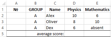
In the cells D5 and E5 we introduce the functions, that help to receive the average of the grades of achievement in the lessons of English & Mathematics. The cell E4 does not matter, so the result will be calculated from 2 estimates.

Work with the cell D5.
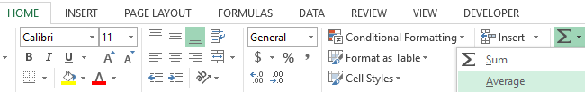
Choose the tool from the drop-down list: «Home» – «Sum» – «Average». In this drop-down list there are frequently used mathematical functions.

The span is determined mechanically, it remains only to press Enter.
The function, that includes the cell D5 now, you need to replicate in the cell E5.

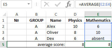
The secondary function in Excel: = AVERAGE () in the cell E5 ignores the text. It will ignore the empty cell also. But if the cell has a value of 0, then the result will change naturally.

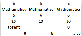
In Excel, there is still the function = AVERAGEA() – the average meaning is an arithmetic number. It differs from the previous one in that:

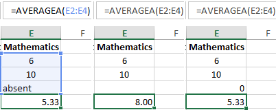
= AVERAGE() – there are skips cells that don`t contain numbers;
= AVERAGEA() – there are skips only empty cells, and accepts text values as 0.

The function of counting the number of values in Excel

In the cells D6 and E6 in our table you need to enter the function of counting the number of numerical values. The function will allow us to learn the number of grades given.
Go to the cell D6 and pick out the tool from the drop-down list: «Home» – «Sum» – «Number».
This time, the automatic detection of a range of cells is not suitable for us, so you need to fix it to D2:D4. Press Enter after that.
From D6 to the cell E6, you should copy = COUNT () – it need for counting the number of non-empty cells.

COUNT.

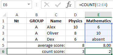
In this example it’s clear, that the function = COUNT() overlooks cells, that don`t comprise number or are empty.

The IF function in Excel

In the cells D7 and E7 you need to introduce a logical function, that will allow us to check whether all students have grades. There is example of IF function:

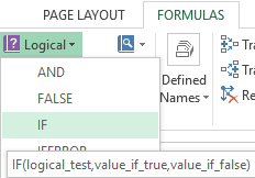
Go to the cell D7, select the tool: «FORMULAS» – «Logical» – «IF».

Fill in the arguments of the function in the dialog box, as you can see in the figure and click OK (note, that the 2-nd link $A$4 is absolute):

IF.

The function from D7 is copied to E7.

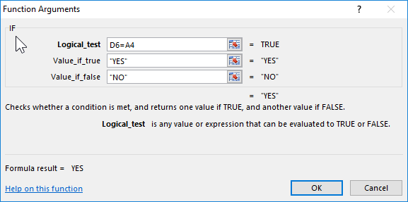
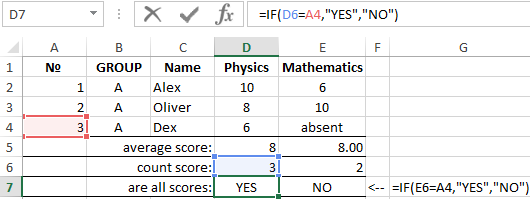
The specification of function arguments: = IF (). There are the number of all students in the cell A4, and in the cell D6 and E6 – the number of estimates. The IF () checks whether D6 and E6 are the same as A4. If functions are the same, we get the answer YES, and if not, the answer is NO.

In logical expression, there are 2 types of references are used for convenience: relative and absolute. This allows us to copy the formula without errors in the results of its calculation.

The notation. The «Formulas» tab provides access only to the most frequently used functions. You may get more by calling the «Functions Wizard» window by clicking on the «Insert function» button at the beginning of the formula line. Or we may press SHIFT + F3.

How to round numbers in Excel

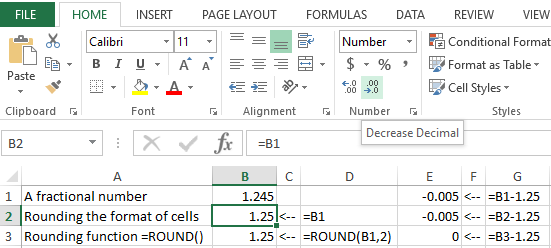
The = ROUND () is more accurate and useful than rounding by using a cell format. This is easily seen in practice.

Make the original chart as shown in the picture:

ROUND.

The cell B2 you need format so, that only 2 decimal places are displayed. This can be done using the «Format cells» dialog box or the tool located on the «HOME» tab – «Decrease Decimal».

In the column C you should add the subtraction formula of 1.25 from the values of column B: =B-1.25.

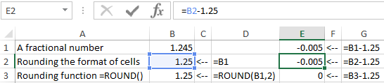
Now you know how to use the ROUND function in Excel.

The description of function arguments =ROUND():

The first reason – is the cell reference to the value to be rounded.
The second reason – is the number of symbols after point, that need to left after rounding.

Attention! The formatting cells only displays rounding, but does not change the value, and = ROUND () – rounds the value. Therefore, for calculations and computations, you need to use the function = ROUND (), inasmuch formatting of the cells will result in erroneous values in the meanings.

Источник

The complete Excel Functions list includes lookup, logic, date and time, text, information, and math functions with examples. Excel Functions are built-in presets, so Excel functions are hard-coded formulas with short, user-friendly names.

The list contains 300+ built-in Excel functions. Furthermore, look at the library of useful advanced functions (UDFs). If you want to jump to a specific category, use the list below; else, use the Search box for the latest tutorials.

User-defined functions (must-have)
Logical
Text
Lookup
Date and Time

Dynamic array
Information
Math
Statistical
Financial

Excel Function List

Logical

The functions below use logical tests and logical operators to evaluate a formula. Learn more about Boolean expressions.

LOOKUP

Here is the list of lookup functions in Excel. Of course, we already know that XLOOKUP changes everything. But it is worth keeping in mind the older lookup functions too.

User-defined functions

UDFs are advanced functions.

Date and Time

Date and Time functions help you create calculations based on dates and times.

Text

Text functions in Excel enable you to perform various calculations using strings.

Dynamic Array

Dynamic Arrays are resizable arrays. From now, Excel calculates the array automatically and returns values into multiple cells based on a formula entered in a single cell.

Information

Take a quick overview of information functions in Excel.

Math

Math Functions are great.

Math – Part 2

Financial

Use financial functions if you want.

Financial – Part 2

Statistical

Statistical – Part 2

Trigonometry

Engineering

Database

How to use Excel Functions?

To use a function, type an equal sign (=) in the formula bar or the cell to enter a function you want to use. After that, enter the function’s name and the arguments. There are custom functions in Excel, user-defined functions. If you want to learn more about how to solve complex tasks using UDFs, read our guide.

Источник

Date and Time Functions

NOW and TODAY

DAY, MONTH, YEAR, and DATE

HOUR, MINUTE, SECOND, and TIME

DATEDIF and YEARFRAC

EDATE and EOMONTH

WORKDAY and NETWORKDAYS

WEEKDAY and WEEKNUM

Engineering

CONVERT

Information Functions

ISBLANK, ISERROR, ISNUMBER, and ISFORMULA

Logical Functions

AND, OR and NOT

IFERROR and IFNA

IF and IFS functions

Lookup and Reference Functions

VLOOKUP and HLOOKUP

INDEX and MATCH

LOOKUP

ROW and COLUMN

ROWS and COLUMNS

HYPERLINK

GETPIVOTDATA

CHOOSE

TRANSPOSE

OFFSET

INDIRECT

STATISTICAL Functions

COUNT and COUNTA

COUNTIF and COUNTIFS

SUM, SUMIF, SUMIFS

AVERAGE, AVERAGEIF, and AVERAGEIFS

MIN, MAX, LARGE, SMALL

MINIFS, MAXIFS

MODE

RANK

MATH Functions

ABS

RAND and RANDBETWEEN

ROUND, ROUNDUP, ROUNDDOWN, INT

MROUND, CEILING, FLOOR

MOD

SUMPRODUCT

SUBTOTAL

AGGREGATE

TEXT Functions

LEFT, RIGHT, MID

LEN

FIND, SEARCH

REPLACE, SUBSTITUTE

CODE, CHAR

TRIM, CLEAN

CONCAT, TEXTJOIN, CONCATENATE

EXACT

UPPER, LOWER, PROPER

TEXT

Dynamic Array functions

Quick navigation

Excel Functions – Date and Time

Excel Functions – Logical

Excel Functions – Lookup & Reference

Excel Functions – Math

Excel Functions – Statistics

​Excel Functions – Text Functions

Excel Functions – Info

Excel Functions – Financial

VBA Functions

The function of calculating the average number

The function of counting the number of values in Excel

The IF function in Excel

How to round numbers in Excel

Excel Function List

Logical

LOOKUP

User-defined functions

Date and Time

Text

Dynamic Array

Information

Excel Functions – Text Functions