Help to use excel

Learn from live instructors

Microsoft offers live coaching to help your learn excel formulas, tip and more to save you time and to take your skills to the next level.

Get started now

Explore Excel

Find Excel templates

Bring your ideas to life and streamline your work by starting with professionally designed, fully customizable templates from Microsoft Create.

Browse templates

Analyze Data

Ask questions about your data without having to write complicated formulas. Not available in all locales.

Explore your data

Plan and track your health

Tackle your health and fitness goals, stay on track of your progress, and be your best self with help from Excel.

Get healthy

Support for Excel 2013 has ended

Learn what end of Excel 2013 support means for you and find out how you can upgrade to Microsoft 365.

Get the details

Trending topics

Sometimes, Excel seems too good to be true. All I have to do is enter a formula, and pretty much anything I’d ever need to do manually can be done automatically.

Need to merge two sheets with similar data? Excel can do it.

Need to do simple math? Excel can do it.

Need to combine information in multiple cells? Excel can do it.

In this post, I’ll go over the best tips, tricks, and shortcuts you can use right now to take your Excel game to the next level. No advanced Excel knowledge required.

What is Excel?

Microsoft Excel is powerful data visualization and analysis software, which uses spreadsheets to store, organize, and track data sets with formulas and functions. Excel is used by marketers, accountants, data analysts, and other professionals. It’s part of the Microsoft Office suite of products. Alternatives include Google Sheets and Numbers. 

Find more Excel alternatives here.

Excel is primarily used for creating financial documents because of its strong computational powers. You’ll often find the software in accounting offices and teams because it allows accountants to automatically see sums, averages, and totals. With Excel, they can easily make sense of their business’ data.

While Excel is primarily known as an accounting tool, professionals in any field can use its features and formulas — especially marketers — because it can be used for tracking any type of data. It removes the need to spend hours and hours counting cells or copying and pasting performance numbers. Excel typically has a shortcut or quick fix that speeds up the process.

You can also download Excel templates below for all of your marketing needs. 

After you download the templates, it’s time to start using the software. Let’s cover the basics first.

Excel Basics

If you’re just starting out with Excel, there are a few basic commands that we suggest you become familiar with. These are things like:

• Creating a new spreadsheet from scratch.
• Executing basic computations like adding, subtracting, multiplying, and dividing.
• Writing and formatting column text and titles.
• Using Excel’s auto-fill features.
• Adding or deleting single columns, rows, and spreadsheets. (Below, we’ll get into how to add things like multiple columns and rows.)
• Keeping column and row titles visible as you scroll past them in a spreadsheet, so that you know what data you’re filling as you move further down the document.
• Sorting your data in alphabetical order. 

Let’s explore a few of these more in-depth. 

For instance, why does auto-fill matter? 

If you have any basic Excel knowledge, it’s likely you already know this quick trick. But to cover our bases, allow me to show you the glory of autofill. This lets you quickly fill adjacent cells with several types of data, including values, series, and formulas.

There are multiple ways to deploy this feature, but the fill handle is among the easiest. Select the cells you want to be the source, locate the fill handle in the lower-right corner of the cell, and either drag the fill handle to cover cells you want to fill or just double click:

Similarly, sorting is an important feature you’ll want to know when organizing your data in Excel. 

Sometimes you may have a list of data that has no organization whatsoever. Maybe you exported a list of your marketing contacts or blog posts. Whatever the case may be, Excel’s sort feature will help you alphabetize any list.

Click on the data in the column you want to sort. Then click on the «Data» tab in your toolbar and look for the «Sort» option on the left. If the «A» is on top of the «Z,» you can just click on that button once. If the «Z» is on top of the «A,» click on the button twice. When the «A» is on top of the «Z,» that means your list will be sorted in alphabetical order. However, when the «Z» is on top of the «A,» that means your list will be sorted in reverse alphabetical order.

Let’s explore more of the basics of Excel (along with advanced features) next. 

To use Excel, you only need to input the data into the rows and columns. And then you’ll use formulas and functions to turn that data into insights. 

We’re going to go over the best formulas and functions you need to know. But first, let’s take a look at the types of documents you can create using the software. That way, you have an overarching understanding of how you can use Excel in your day-to-day. 

Documents You Can Create in Excel

Not sure how you can actually use Excel in your team? Here is a list of documents you can create:

• Income Statements: You can use an Excel spreadsheet to track a company’s sales activity and financial health.
• Balance Sheets: Balance sheets are among the most common types of documents you can create with Excel. It allows you to get a holistic view of a company’s financial standing.
• Calendar: You can easily create a spreadsheet monthly calendar to track events or other date-sensitive information.

Here are some documents you can create specifically for marketers.

• Marketing Budgets: Excel is a strong budget-keeping tool. You can create and track marketing budgets, as well as spend, using Excel. If you don’t want to create a document from scratch, download our marketing budget templates for free.
• Marketing Reports: If you don’t use a marketing tool such as Marketing Hub, you might find yourself in need of a dashboard with all of your reports. Excel is an excellent tool to create marketing reports. Download free Excel marketing reporting templates here.
• Editorial Calendars: You can create editorial calendars in Excel. The tab format makes it extremely easy to track your content creation efforts for custom time ranges. Download a free editorial content calendar template here.
• Traffic and Leads Calculator: Because of its strong computational powers, Excel is an excellent tool to create all sorts of calculators — including one for tracking leads and traffic. Click here to download a free premade lead goal calculator.

This is only a small sampling of the types of marketing and business documents you can create in Excel. We’ve created an extensive list of Excel templates you can use right now for marketing, invoicing, project management, budgeting, and more.

In the spirit of working more efficiently and avoiding tedious, manual work, here are a few Excel formulas and functions you’ll need to know.

Excel Formulas

It’s easy to get overwhelmed by the wide range of Excel formulas that you can use to make sense out of your data. If you’re just getting started using Excel, you can rely on the following formulas to carry out some complex functions — without adding to the complexity of your learning path.

• Equal sign: Before creating any formula, you’ll need to write an equal sign (=) in the cell where you want the result to appear.
• Addition: To add the values of two or more cells, use the + sign. Example: =C5+D3.
• Subtraction: To subtract the values of two or more cells, use the — sign. Example: =C5-D3.
• Multiplication: To multiply the values of two or more cells, use the * sign. Example: =C5*D3.
• Division: To divide the values of two or more cells, use the / sign. Example: =C5/D3.

Putting all of these together, you can create a formula that adds, subtracts, multiplies, and divides all in one cell. Example: =(C5-D3)/((A5+B6)*3).

For more complex formulas, you’ll need to use parentheses around the expressions to avoid accidentally using the PEMDAS order of operations. Keep in mind that you can use plain numbers in your formulas.

Excel Functions

Excel functions automate some of the tasks you would use in a typical formula. For instance, instead of using the + sign to add up a range of cells, you’d use the SUM function. Let’s look at a few more functions that will help automate calculations and tasks.

• SUM: The SUM function automatically adds up a range of cells or numbers. To complete a sum, you would input the starting cell and the final cell with a colon in between. Here’s what that looks like: SUM(Cell1:Cell2). Example: =SUM(C5:C30).
• AVERAGE: The AVERAGE function averages out the values of a range of cells. The syntax is the same as the SUM function: AVERAGE(Cell1:Cell2). Example: =AVERAGE(C5:C30).
• IF: The IF function allows you to return values based on a logical test. The syntax is as follows: IF(logical_test, value_if_true, [value_if_false]). Example: =IF(A2>B2,»Over Budget»,»OK»).
• VLOOKUP: The VLOOKUP function helps you search for anything on your sheet’s rows. The syntax is: VLOOKUP(lookup value, table array, column number, Approximate match (TRUE) or Exact match (FALSE)). Example: =VLOOKUP([@Attorney],tbl_Attorneys,4,FALSE).
• INDEX: The INDEX function returns a value from within a range. The syntax is as follows: INDEX(array, row_num, [column_num]).
• MATCH: The MATCH function looks for a certain item in a range of cells and returns the position of that item. It can be used in tandem with the INDEX function. The syntax is: MATCH(lookup_value, lookup_array, [match_type]).
• COUNTIF: The COUNTIF function returns the number of cells that meet a certain criteria or have a certain value. The syntax is: COUNTIF(range, criteria). Example: =COUNTIF(A2:A5,»London»).

Okay, ready to get into the nitty-gritty? Let’s get to it. (And to all the Harry Potter fans out there … you’re welcome in advance.)

Note: The GIFs and visuals are from a previous version of Excel. When applicable, the copy has been updated to provide instruction for users of both newer and older Excel versions.

1. Use Pivot tables to recognize and make sense of data.

Pivot tables are used to reorganize data in a spreadsheet. They won’t change the data that you have, but they can sum up values and compare different information in your spreadsheet, depending on what you’d like them to do.

Let’s take a look at an example. Let’s say I want to take a look at how many people are in each house at Hogwarts. You may be thinking that I don’t have too much data, but for longer data sets, this will come in handy.

To create the Pivot Table, I go to Data > Pivot Table. If you’re using the most recent version of Excel, you’d go to Insert > Pivot Table. Excel will automatically populate your Pivot Table, but you can always change around the order of the data. Then, you have four options to choose from.

• Report Filter: This allows you to only look at certain rows in your dataset. For example, if I wanted to create a filter by house, I could choose to only include students in Gryffindor instead of all students.
• Column Labels: These would be your headers in the dataset.
• Row Labels: These could be your rows in the dataset. Both Row and Column labels can contain data from your columns (e.g. First Name can be dragged to either the Row or Column label — it just depends on how you want to see the data.)
• Value: This section allows you to look at your data differently. Instead of just pulling in any numeric value, you can sum, count, average, max, min, count numbers, or do a few other manipulations with your data. In fact, by default, when you drag a field to Value, it always does a count.

Since I want to count the number of students in each house, I’ll go to the Pivot table builder and drag the House column to both the Row Labels and the Values. This will sum up the number of students associated with each house.

2. Add more than one row or column.

As you play around with your data, you might find you’re constantly needing to add more rows and columns. Sometimes, you may even need to add hundreds of rows. Doing this one-by-one would be super tedious. Luckily, there’s always an easier way.

To add multiple rows or columns in a spreadsheet, highlight the same number of preexisting rows or columns that you want to add. Then, right-click and select «Insert.»

In the example below, I want to add an additional three rows. By highlighting three rows and then clicking insert, I’m able to add an additional three blank rows into my spreadsheet quickly and easily.

3. Use filters to simplify your data.

When you’re looking at very large data sets, you don’t usually need to be looking at every single row at the same time. Sometimes, you only want to look at data that fit into certain criteria.

That’s where filters come in.

Filters allow you to pare down your data to only look at certain rows at one time. In Excel, a filter can be added to each column in your data — and from there, you can then choose which cells you want to view at once.

Let’s take a look at the example below. Add a filter by clicking the Data tab and selecting «Filter.» Clicking the arrow next to the column headers and you’ll be able to choose whether you want your data to be organized in ascending or descending order, as well as which specific rows you want to show.

In my Harry Potter example, let’s say I only want to see the students in Gryffindor. By selecting the Gryffindor filter, the other rows disappear.

Pro Tip: Copy and paste the values in the spreadsheet when a Filter is on to do additional analysis in another spreadsheet.

4. Remove duplicate data points or sets.

Larger data sets tend to have duplicate content. You may have a list of multiple contacts in a company and only want to see the number of companies you have. In situations like this, removing the duplicates comes in quite handy.

To remove your duplicates, highlight the row or column that you want to remove duplicates of. Then, go to the Data tab and select «Remove Duplicates» (which is under the Tools subheader in the older version of Excel). A pop-up will appear to confirm which data you want to work with. Select «Remove Duplicates,» and you’re good to go.

You can also use this feature to remove an entire row based on a duplicate column value. So if you have three rows with Harry Potter’s information and you only need to see one, then you can select the whole dataset and then remove duplicates based on email. Your resulting list will have only unique names without any duplicates.

5. Transpose rows into columns.

When you have rows of data in your spreadsheet, you might decide you actually want to transform the items in one of those rows into columns (or vice versa). It would take a lot of time to copy and paste each individual header — but what the transpose feature allows you to do is simply move your row data into columns, or the other way around.

Start by highlighting the column that you want to transpose into rows. Right-click it, and then select «Copy.» Next, select the cells on your spreadsheet where you want your first row or column to begin. Right-click on the cell, and then select «Paste Special.» A module will appear — at the bottom, you’ll see an option to transpose. Check that box and select OK. Your column will now be transferred to a row or vice-versa.

On newer versions of Excel, a drop-down will appear instead of a pop-up.

6. Split up text information between columns.

What if you want to split out information that’s in one cell into two different cells? For example, maybe you want to pull out someone’s company name through their email address. Or perhaps you want to separate someone’s full name into a first and last name for your email marketing templates.

Thanks to Excel, both are possible. First, highlight the column that you want to split up. Next, go to the Data tab and select «Text to Columns.» A module will appear with additional information.

First, you need to select either «Delimited» or «Fixed Width.»

• «Delimited» means you want to break up the column based on characters such as commas, spaces, or tabs.
• «Fixed Width» means you want to select the exact location on all the columns that you want the split to occur.

In the example case below, let’s select «Delimited» so we can separate the full name into first name and last name.

Then, it’s time to choose the Delimiters. This could be a tab, semi-colon, comma, space, or something else. («Something else» could be the «@» sign used in an email address, for example.) In our example, let’s choose the space. Excel will then show you a preview of what your new columns will look like.

When you’re happy with the preview, press «Next.» This page will allow you to select Advanced Formats if you choose to. When you’re done, click «Finish.»

7. Use formulas for simple calculations.

In addition to doing pretty complex calculations, Excel can help you do simple arithmetic like adding, subtracting, multiplying, or dividing any of your data.

• To add, use the + sign.
• To subtract, use the — sign.
• To multiply, use the * sign.
• To divide, use the / sign.

You can also use parentheses to ensure certain calculations are done first. In the example below (10+10*10), the second and third 10 were multiplied together before adding the additional 10. However, if we made it (10+10)*10, the first and second 10 would be added together first.

8. Get the average of numbers in your cells.

If you want the average of a set of numbers, you can use the formula =AVERAGE(Cell1:Cell2). If you want to sum up a column of numbers, you can use the formula =SUM(Cell1:Cell2).

9. Use conditional formatting to make cells automatically change color based on data.

Conditional formatting allows you to change a cell’s color based on the information within the cell. For example, if you want to flag certain numbers that are above average or in the top 10% of the data in your spreadsheet, you can do that. If you want to color code commonalities between different rows in Excel, you can do that. This will help you quickly see information that is important to you.

To get started, highlight the group of cells you want to use conditional formatting on. Then, choose «Conditional Formatting» from the Home menu and select your logic from the dropdown. (You can also create your own rule if you want something different.) A window will pop up that prompts you to provide more information about your formatting rule. Select «OK» when you’re done, and you should see your results automatically appear.

10. Use the IF Excel formula to automate certain Excel functions.

Sometimes, we don’t want to count the number of times a value appears. Instead, we want to input different information into a cell if there is a corresponding cell with that information.

For example, in the situation below, I want to award ten points to everyone who belongs in the Gryffindor house. Instead of manually typing in 10’s next to each Gryffindor student’s name, I can use the IF Excel formula to say that if the student is in Gryffindor, then they should get ten points.

The formula is: IF(logical_test, value_if_true, [value_if_false])

Example Shown Below: =IF(D2=»Gryffindor»,»10″,»0″)

In general terms, the formula would be IF(Logical Test, value of true, value of false). Let’s dig into each of these variables.

• Logical_Test: The logical test is the «IF» part of the statement. In this case, the logic is D2=»Gryffindor» because we want to make sure that the cell corresponding with the student says «Gryffindor.» Make sure to put Gryffindor in quotation marks here.
• Value_if_True: This is what we want the cell to show if the value is true. In this case, we want the cell to show «10» to indicate that the student was awarded the 10 points. Only use quotation marks if you want the result to be text instead of a number.
• Value_if_False: This is what we want the cell to show if the value is false. In this case, for any student not in Gryffindor, we want the cell to show «0». Only use quotation marks if you want the result to be text instead of a number.

Note: In the example above, I awarded 10 points to everyone in Gryffindor. If I later wanted to sum the total number of points, I wouldn’t be able to because the 10’s are in quotes, thus making them text and not a number that Excel can sum.

The real power of the IF function comes when you string multiple IF statements together, or nest them. This allows you to set multiple conditions, get more specific results, and ultimately organize your data into more manageable chunks.

Ranges are one way to segment your data for better analysis. For example, you can categorize data into values that are less than 10, 11 to 50, or 51 to 100. Here’s how that looks in practice: 

=IF(B3<11,“10 or less”,IF(B3<51,“11 to 50”,IF(B3<100,“51 to 100”)))

It can take some trial-and-error, but once you have the hang of it, IF formulas will become your new Excel best friend.

11. Use dollar signs to keep one cell’s formula the same regardless of where it moves.

Have you ever seen a dollar sign in an Excel formula? When used in a formula, it isn’t representing an American dollar; instead, it makes sure that the exact column and row are held the same even if you copy the same formula in adjacent rows.

You see, a cell reference — when you refer to cell A5 from cell C5, for example — is relative by default. In that case, you’re actually referring to a cell that’s five columns to the left (C minus A) and in the same row (5). This is called a relative formula. When you copy a relative formula from one cell to another, it’ll adjust the values in the formula based on where it’s moved. But sometimes, we want those values to stay the same no matter whether they’re moved around or not — and we can do that by turning the formula into an absolute formula.

To change the relative formula (=A5+C5) into an absolute formula, we’d precede the row and column values by dollar signs, like this: (=$A$5+$C$5). (Learn more on Microsoft Office’s support page here.)

12. Use the VLOOKUP function to pull data from one area of a sheet to another.

Have you ever had two sets of data on two different spreadsheets that you want to combine into a single spreadsheet?

For example, you might have a list of people’s names next to their email addresses in one spreadsheet, and a list of those same people’s email addresses next to their company names in the other — but you want the names, email addresses, and company names of those people to appear in one place.

I have to combine data sets like this a lot — and when I do, the VLOOKUP is my go-to formula.

Before you use the formula, though, be absolutely sure that you have at least one column that appears identically in both places. Scour your data sets to make sure the column of data you’re using to combine your information is exactly the same, including no extra spaces.

The formula: =VLOOKUP(lookup value, table array, column number, Approximate match (TRUE) or Exact match (FALSE))

The formula with variables from our example below: =VLOOKUP(C2,Sheet2!A:B,2,FALSE)

In this formula, there are several variables. The following is true when you want to combine information in Sheet 1 and Sheet 2 onto Sheet 1.

• Lookup Value: This is the identical value you have in both spreadsheets. Choose the first value in your first spreadsheet. In the example that follows, this means the first email address on the list, or cell 2 (C2).
• Table Array: The table array is the range of columns on Sheet 2 you’re going to pull your data from, including the column of data identical to your lookup value (in our example, email addresses) in Sheet 1 as well as the column of data you’re trying to copy to Sheet 1. In our example, this is «Sheet2!A:B.» «A» means Column A in Sheet 2, which is the column in Sheet 2 where the data identical to our lookup value (email) in Sheet 1 is listed. The «B» means Column B, which contains the information that’s only available in Sheet 2 that you want to translate to Sheet 1.
• Column Number: This tells Excel which column the new data you want to copy to Sheet 1 is located in. In our example, this would be the column that «House» is located in. «House» is the second column in our range of columns (table array), so our column number is 2. [Note: Your range can be more than two columns. For example, if there are three columns on Sheet 2 — Email, Age, and House — and you still want to bring House onto Sheet 1, you can still use a VLOOKUP. You just need to change the «2» to a «3» so it pulls back the value in the third column: =VLOOKUP(C2:Sheet2!A:C,3,false).]
• Approximate Match (TRUE) or Exact Match (FALSE): Use FALSE to ensure you pull in only exact value matches. If you use TRUE, the function will pull in approximate matches.

In the example below, Sheet 1 and Sheet 2 contain lists describing different information about the same people, and the common thread between the two is their email addresses. Let’s say we want to combine both datasets so that all the house information from Sheet 2 translates over to Sheet 1.

So when we type in the formula =VLOOKUP(C2,Sheet2!A:B,2,FALSE), we bring all the house data into Sheet 1.

Keep in mind that VLOOKUP will only pull back values from the second sheet that are to the right of the column containing your identical data. This can lead to some limitations, which is why some people prefer to use the INDEX and MATCH functions instead.

13. Use INDEX and MATCH formulas to pull data from horizontal columns.

Like VLOOKUP, the INDEX and MATCH functions pull in data from another dataset into one central location. Here are the main differences:

• VLOOKUP is a much simpler formula. If you’re working with large data sets that would require thousands of lookups, using the INDEX and MATCH function will significantly decrease load time in Excel.
• The INDEX and MATCH formulas work right-to-left, whereas VLOOKUP formulas only work as a left-to-right lookup. In other words, if you need to do a lookup that has a lookup column to the right of the results column, then you’d have to rearrange those columns in order to do a VLOOKUP. This can be tedious with large datasets and/or lead to errors.

So if I want to combine information in Sheet 1 and Sheet 2 onto Sheet 1, but the column values in Sheets 1 and 2 aren’t the same, then to do a VLOOKUP, I would need to switch around my columns. In this case, I’d choose to do an INDEX and MATCH instead.

Let’s look at an example. Let’s say Sheet 1 contains a list of people’s names and their Hogwarts email addresses, and Sheet 2 contains a list of people’s email addresses and the Patronus that each student has. (For the non-Harry Potter fans out there, every witch or wizard has an animal guardian called a «Patronus» associated with him or her.) The information that lives in both sheets is the column containing email addresses, but this email address column is in different column numbers on each sheet. I’d use the INDEX and MATCH formulas instead of VLOOKUP so I wouldn’t have to switch any columns around.

So what’s the formula, then? The formula is actually the MATCH formula nested inside the INDEX formula. You’ll see I differentiated the MATCH formula using a different color here.

The formula: =INDEX(table array, MATCH formula)

This becomes: =INDEX(table array, MATCH (lookup_value, lookup_array))

The formula with variables from our example below: =INDEX(Sheet2!A:A,(MATCH(Sheet1!C:C,Sheet2!C:C,0)))

Here are the variables:

• Table Array: The range of columns on Sheet 2 containing the new data you want to bring over to Sheet 1. In our example, «A» means Column A, which contains the «Patronus» information for each person.
• Lookup Value: This is the column in Sheet 1 that contains identical values in both spreadsheets. In the example that follows, this means the «email» column on Sheet 1, which is Column C. So: Sheet1!C:C.
• Lookup Array: This is the column in Sheet 2 that contains identical values in both spreadsheets. In the example that follows, this refers to the «email» column on Sheet 2, which happens to also be Column C. So: Sheet2!C:C.

Once you have your variables straight, type in the INDEX and MATCH formulas in the top-most cell of the blank Patronus column on Sheet 1, where you want the combined information to live.

14. Use the COUNTIF function to make Excel count words or numbers in any range of cells.

Instead of manually counting how often a certain value or number appears, let Excel do the work for you. With the COUNTIF function, Excel can count the number of times a word or number appears in any range of cells.

For example, let’s say I want to count the number of times the word «Gryffindor» appears in my data set.

The formula: =COUNTIF(range, criteria)

The formula with variables from our example below: =COUNTIF(D:D,»Gryffindor»)

In this formula, there are several variables:

• Range: The range that we want the formula to cover. In this case, since we’re only focusing on one column, we use «D:D» to indicate that the first and last column are both D. If I were looking at columns C and D, I would use «C:D.»
• Criteria: Whatever number or piece of text you want Excel to count. Only use quotation marks if you want the result to be text instead of a number. In our example, the criteria is «Gryffindor.»

Simply typing in the COUNTIF formula in any cell and pressing «Enter» will show me how many times the word «Gryffindor» appears in the dataset.

15. Combine cells using &.

Databases tend to split out data to make it as exact as possible. For example, instead of having a column that shows a person’s full name, a database might have the data as a first name and then a last name in separate columns. Or, it may have a person’s location separated by city, state, and zip code. In Excel, you can combine cells with different data into one cell by using the «&» sign in your function.

The formula with variables from our example below: =A2&» «&B2

Let’s go through the formula together using an example. Pretend we want to combine first names and last names into full names in a single column. To do this, we’d first put our cursor in the blank cell where we want the full name to appear. Next, we’d highlight one cell that contains a first name, type in an «&» sign, and then highlight a cell with the corresponding last name.

But you’re not finished — if all you type in is =A2&B2, then there will not be a space between the person’s first name and last name. To add that necessary space, use the function =A2&» «&B2. The quotation marks around the space tell Excel to put a space in between the first and last name.

To make this true for multiple rows, simply drag the corner of that first cell downward as shown in the example.

16. Add checkboxes.

If you’re using an Excel sheet to track customer data and want to oversee something that isn’t quantifiable, you could insert checkboxes into a column.

For example, if you’re using an Excel sheet to manage your sales prospects and want to track whether you called them in the last quarter, you could have a «Called this quarter?» column and check off the cells in it when you’ve called the respective client.

Here’s how to do it.

Highlight a cell you’d like to add checkboxes to in your spreadsheet. Then, click DEVELOPER. Then, under FORM CONTROLS, click the checkbox or the selection circle highlighted in the image below.

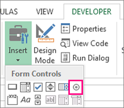
Once the box appears in the cell, copy it, highlight the cells you also want it to appear in, and then paste it.

17. Hyperlink a cell to a website.

If you’re using your sheet to track social media or website metrics, it can be helpful to have a reference column with the links each row is tracking. If you add a URL directly into Excel, it should automatically be clickable. But, if you have to hyperlink words, such as a page title or the headline of a post you’re tracking, here’s how.

Highlight the words you want to hyperlink, then press Shift K. From there a box will pop up allowing you to place the hyperlink URL. Copy and paste the URL into this box and hit or click Enter.

If the key shortcut isn’t working for any reason, you can also do this manually by highlighting the cell and clicking Insert > Hyperlink.

18. Add drop-down menus.

Sometimes, you’ll be using your spreadsheet to track processes or other qualitative things. Rather than writing words into your sheet repetitively, such as «Yes», «No», «Customer Stage», «Sales Lead», or «Prospect», you can use dropdown menus to quickly mark descriptive things about your contacts or whatever you’re tracking.

Here’s how to add drop-downs to your cells.

Highlight the cells you want the drop-downs to be in, then click the Data menu in the top navigation and press Validation.

From there, you’ll see a Data Validation Settings box open. Look at the Allow options, then click Lists and select Drop-down List. Check the In-Cell dropdown button, then press OK.

19. Use the format painter. 

As you’ve probably noticed, Excel has a lot of features to make crunching numbers and analyzing your data quick and easy. But if you ever spent some time formatting a sheet to your liking, you know it can get a bit tedious.

Don’t waste time repeating the same formatting commands over and over again. Use the format painter to easily copy the formatting from one area of the worksheet to another. To do so, choose the cell you’d like to replicate, then select the format painter option (paintbrush icon) from the top toolbar.

Excel Keyboard Shortcuts 

Creating reports in Excel is time-consuming enough. How can we spend less time navigating, formatting, and selecting items in our spreadsheet? Glad you asked. There are a ton of Excel shortcuts out there, including some of our favorites listed below.

Create a New Workbook

PC: Ctrl-N | Mac: Command-N

Select Entire Row

PC: Shift-Space | Mac: Shift-Space

Select Entire Column

PC: Ctrl-Space | Mac: Control-Space

Select Rest of Column

PC: Ctrl-Shift-Down/Up | Mac: Command-Shift-Down/Up

Select Rest of Row

PC: Ctrl-Shift-Right/Left | Mac: Command-Shift-Right/Left

Add Hyperlink

PC: Ctrl-K | Mac: Command-K

Open Format Cells Window

PC: Ctrl-1 | Mac: Command-1

Autosum Selected Cells

PC: Alt-= | Mac: Command-Shift-T

Other Excel Help Resources

• How to Make a Chart or Graph in Excel [With Video Tutorial]
• Design Tips to Create Beautiful Excel Charts and Graphs
• Totally Free Microsoft Excel Templates That Make Marketing Easier
• How to Learn Excel Online: Free and Paid Resources for Excel Training

Use Excel to Automate Processes in Your Team

Even if you’re not an accountant, you can still use Excel to automate tasks and processes in your team. With the tips and tricks we shared in this post, you’ll be sure to use Excel to its fullest extent and get the most out of the software to grow your business.

Editor’s Note: This post was originally published in August 2017 but has been updated for comprehensiveness.

One of the FASTEST ways to Learn Excel is to learn some of the Excel TIPS and TRICKS, period and if you learn a single Excel tip a day you can learn 30 new things in a month.

But you must have a list that you can refer to every day instead of searching here and there. Well, I’m super PROUD to say that this is the most comprehensive list with all the basic and advanced tips that you can find on the INTERNET.

In this LIST, I have covered 300+ Excel TIPS and TRICKS which you can learn to Level Up your Excel Skills.

1. Add Serial Numbers

If you work with large data then it’s better to add a serial number column to it. For me, the best way to do this is to apply the table (Control + T) to the data and then add 1 in the above serial number, just like below.

To do this, you simply need to add 1 to the first cell of the column and then create a formula to add 1 to the above cell’s value. As you are using a table, whenever you create a new entry in the table, Excel will automatically drop down the formula and you will get the serial number.

2. Insert Current Date and Time

The best way to insert the current date and time is to use the NOW function which takes the date and time from the system and returns it.

The only problem with this function is it’s volatile, and whenever you recalculate something it updates its value. And if you don’t want to do this, the best way is to convert it to hard value. You can also use the below VBA code.

Sub timestamp()
Dim ts As Date
With Selection
.Value = Now
.NumberFormat = "m/d/yyyy h:mm:ss AM/PM"
End With
End Sub

Or these methods to insert a timestamp in a cell.

3. Select Non-Continues Cells

Normally we all do it this way, hold the control key, and select cells one by one. But I have found that there is a far better way for this. All you have to do is, select the first cell and then press SHIFT + F8.

This gives you add or remove selection mode in which you can select cells just by selecting them.

4. Sort Buttons

If you deal with data that needs to sort frequently then it’s better to add a button to the quick access toolbar (if it’s not there already).

All you need to do is click on the down arrow on the quick access toolbar and then select “Sort Ascending” and “Sort Descending”. It adds both buttons to the QAT.

5. Move Data

I’m sure you think about copy-paste but you can also use drag-drop for this.

Simply select the range where you have data and then click on the border of the selection. By holding it move to the place where you need to put it.

6. Status Bar

The status bar is always there but we hardly use it to the full. If you right-click on it, you can see there are a lot of options you can add.

7. Clipboard

There is a problem with normal copy-paste that you can only use a single value at a time.

But here is the kicker: When you copy a value, it goes to the clipboard and if you open the clipboard you can paste all the values which you have copied. To open a clipboard, click on the go to Home Tab ➜ Editing and then click on the down arrow.

It will open the clipboard on the left side, and you can paste values from there.

8. Bullet Points

The easiest way to insert bullet points in Excel is by using custom formatting and here are the steps for this:

1. Press Ctrl + 1 and you will get the “Format Cell” dialogue box.
2. Under the number tab, select custom.
3. In the input bar, enter the following formatting.
   1. ● General;● General;● General;● General
4. In the end, click OK.

Now, whenever you enter a value in the cell Excel will add a bullet before that.

9. Worksheet Copy

To create a copy of a worksheet in the same workbook drag and drop in the best way.

You just need to click and hold the mouse on the sheet’s name tab and then drag and drop it, to the left or right, where you want to create a copy.

10. Undo-Redo

Just like sort buttons you can also add undo and redo buttons to the QAT. The best part about those buttons is you can use them to undo a particular activity without pressing the shortcut key again and again.

More Basic Tips: Delta Symbol | Degree Symbol | Formula to Value | Concatenate a Range of Cells | Insert a Check Mark Symbol in Excel | Convert Negative Number into Positive | Highlight Blank Cells in Excel

11. AutoFormat

If you deal with financial data, then auto format can be one of your best tools. It simply applies the format to small as well as large data sets (especially when data is in tabular form).

1. First of all, you need to add it to the quick access toolbar (here are the steps).
2. After that, whenever you need to apply the format, just select the data where you want to apply it and click on the AUTO FORMAT button from the quick access toolbar.
3. It will show you a window to select the formatting type and after selecting that click OK.

The AUTOFORMAT is a combination of six different formattings and you have the option to disable any of them while applying it.

12. Format Painter

The simple idea with the format painter is to copy and paste formatting from one section to another. Let’s say you have specific formatting (Font Style and Color, Background Color to a Cell, Bold, Border, etc.) in the range B2:D7, and with format painter, you can copy that formatting to range B9: D14 with a click.

1. First of all, select the range B2:D7.
2. After that, go to the Home Tab ➜ Clipboard and then click on “Format Painter”.
3. Now, select cell C1 and it will automatically apply the formatting on B9: D14.

The format painter is fast and makes it easy to apply to format from one section to another.

Related: Format Painter Shortcut

13. Cell Message

Let’s say you need to add a specific message to a cell, like “Don’t delete the value”, “enter your name” or something like that.

In this case, you can add a cell message for that particular cell. When the user will select that cell, it will show the message you have specified. Here are the steps to do this:

1. First, select the cell to which you want to add a message.
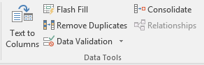
2. After that, go to the Data Tab ➜ Data Tools ➜ Data Validation ➜ Data Validation.
3. In the data validation window, go to the Input Message tab.
4. Enter the title, and message, and make sure to tick mark “Show input message when the cell is selected”.
5. In the end, click OK.

Once the message is shown you can drag and drop it to change its position.

14. Strikethrough

Unlike Word, in Excel, there is no option on the ribbon to apply strikethrough. But I have figured out that there are 5 ways to do it and the easiest of all of them is a keyboard shortcut.

All you need to do is select the cell where you want to apply the strikethrough and use the below keyboard shortcut.

Ctrl + 5

And if you are using MAC then:

⌘ + ⇧ + X

Quick Note: You can use the same shortcut keys if you need to do this for partial text.

15. Add Barcode

It is one of those secret tips that most Excel users are unaware of. To create a bar-code in Excel all you need to do is install this bar-code font from ID-AUTOMATIC.

Once you install this font, you will have to type the number in a cell for which you want to create a bar code and then apply the font style.

learn more about this tip

16. Month Name

Alright, let’s say you have a date in a cell, and you want that date to show as a month or a year. For this, you can apply custom formatting.

• First, select the cell with a date and open formatting options (use Ctrl + 1).
• Select the “Custom” option and add “MMM” or “MMMMMM” for the month or “YYYY” for the year format.
• In the end, click OK.

Custom formatting just changes the formatting of the cell from date to year/month, but the value remains the same.

17. Highlight Blank Cells

When you work with large data sheets it’s hard to identify the blank cells. So, the best way is to highlight them by applying a cell color.

• First, select all the data from the worksheet using the shortcut key Ctrl + A.

• After that, go to Home Tab ➜ Editing ➜ Find & Select ➜ Go to Special.

• From Go to Special dialog box, select Blank and click OK.

• At this point, you have all the blank cells selected and now apply a cell color using font settings.

…but you can also use conditional formatting for this

18. Font Color with Custom Formatting

In Excel, we can apply custom formatting and in custom formatting, there is an option to use font colors (limited but useful).

For example, if you want to use the Green color for positive numbers and the red color for negative numbers then you need to use the custom format.

[Green]#,###;[Red]-#,###;0;

1. First, select the cells where you want to apply this format.
2. After that open the format option using the keyboard shortcut Ctrl + 1 and go to the “Custom” category and the custom format in the input dialogue box.
3. In the end, click OK.

19. Theme Color

We all have some favorite fonts and colors which we use in Excel. Let’s say you received a file from your colleague and now you want to change the font and colors for the worksheet from that file. The point is, you need to do this one by one for each worksheet and that takes time.

But if you create a custom theme with your favorite colors and fonts then you can change the style of the worksheet with a single click. For this, all you have to do is apply your favorite designs to the tables, colors to the shapes and charts, and font style, and then save it as a custom theme.

1. Go to the Page Layout Tab ➜ Themes ➜ Save Current Theme. It opens a “Save As” dialogue box, names your theme, and saves it.
2. And now, every time you need just one click to change any worksheet style to your custom style.

20. Clear Formatting

This is a simple keyboard shortcut that you can use to clear formatting from a cell or range of cells.

Alt ➜ H ➜ E ➜ F

Or, otherwise, you can also use the clear formatting option from the Home Tab (Home Tab ➜ Editing ➜ Clear ➜ Formats).

21. Sentence Case

In Excel, we have three different functions (LOWER, UPPER, and PROPER) to convert text into different cases. But there is no option to convert a text into a sentence case. Here is the formula which you can use:

=UPPER(LEFT(A1,1))&LOWER(RIGHT(A1,LEN(A1)-1))

This formula converts the first letter of a sentence into capital and the rest all in small (learn how this formula works).

22. Random Numbers

In Excel, there are two specific functions that you can use to generate random numbers. First is RAND which generates random numbers between 0 and 1.

And second is RANDBETWEEN which generates random numbers within the range of two specific numbers.

ALERT: These functions are volatile so whenever you re-calculate your worksheet or hit enter, they update their values so make sure to use them with caution. You can also use RANDBETWEEN to generate random letters and random dates.

23. Count Words

In Excel, there is no specific function to count words. You can count characters with LEN but not words. But, you can use the following formula which can help you to count words from a cell.

=LEN(A1)-LEN(SUBSTITUTE(A1,” “,”))+1

This formula counts the number of spaces from a cell and adds 1 to it after that which equals the total number of words in a cell.

24. Calculate the Age

The best way to calculate a person’s age is by using the DATEDIF. This mysterious function is specifically made to get the difference between a date range.

And the formula will be:

=”Your age is “& DATEDIF(Date-of-Birth,Today(),”y”) &” Year(s), “& DATEDIF(Date-of-Birth,TODAY(),”ym”)& ” MONTH(s) & “& DATEDIF(Date-of-Birth,TODAY(),”md”)& ” Day(s).”

25. Calculate the Ratio

I have figured out that there are four different ways to calculate the ratio in Excel but using a simple divide method is the easiest one. All you need to do is divide the larger number into the smaller ones and concatenate it with a colon and one and here’s the formula you need to use:

=Larger-Number/Smaller-Number&”:”&”1″

This formula divides the larger number by the smaller one so that you can take the smaller number as a base (1).

26. Root of Number

To calculate the square root, cube root, or any root of a number the best way is to use the exponent formula. In the exponent formula, you can specify the Nth number for which you want to calculate the root.

=number^(1/n)

For example, if you want to calculate a square root of 625 then the formula will be:

=625^(1/2)

28. Month’s Last Date

To simply get the last date of a month you can use the following dynamic formula.

=DATE(YEAR(TODAY()),MONTH(TODAY())+1,0)

29. Reverse VLOOKUP

As we all know there is no way to look up to left for a value using VLOOKUP. But if you switch to INDEX MATCH you can look up in any direction.

30. SUMPRODUCT IF

You can use the below formula to create a conditional SUMPRODUCT and product values using a condition.

=SUMPRODUCT(–(C7:C19=C2),E7:E19,F7:F19)

31. Smooth Line

If you love to use a line chart, then you are awesome but it would be more awesome if you use a smooth line in the chart. This will give a smart look to your chart.

1. Select the data line in your chart and right-click on it.
2. Select “Format Data Series”.
3. Go to Fill & Line ➜ Line ➜ Tick mark “Smoothed Line”.

33. Hide Axis Labels

This charting tip is simple but still quite functional. If you don’t want to show axis label values in your chart you can delete them. But the better way is to hide them instead of deleting them. Here are the steps:

1. Select the Horizontal/Vertical axis in the chart.
2. Go to “Format Axis” Labels.
3. In the label position, select “None”.

And again, if you want to show it then just select “Next to axis”.

34. Display Units

If you are dealing with large numbers in your chart, you can change the units for axis values.

1. Select the chart axis of your chart and open the format “Format Axis” options.
2. In axis options, go to “Display Units” where you can select a unit for your axis values.

35. Round Corner

I often use Excel charts with rounded corners and if you like to use round corners too, here are the simple steps.

1. Select your chart and open formatting options.
2. Go to Fill and Line ➜ Borders.
3. In borders sections, tick mark rounded corners.

36. Hide Gap

Let’s say you have a chart with monthly sales in which June has no amount and the cell is empty. You can use the following options for that empty cell.

• Show the gap for the empty cell.
• Use zero.
• Connect data points with the line.

Here are the steps to use these options.

1. Right, click on your chart & select “Select Data”.
2. In the select data window, click on “Hidden and Empty Cell”.
3. Select your desired option from “Show Empty Cell as”.

Make sure to use “Connect data points with the line” (recommended).

38. Chart Template

Let’s say you have a favorite chart formatting you want to apply every time you create a new chart. You can create a chart template to use anytime in the future and the steps are as follow.

• Once you have done with your favorite formatting, right-click on it & select “Save As Template”.

• Using the save as dialog box, save it in the template folder.
• To insert a new one with your favorite template, select it from templates in the insert chart dialog.

39. Default Chart

You can use a shortcut key to insert a chart, but the problem is, it will only insert the default chart, and in Excel, the default chart type is “Column Chart”. So if your favorite chart is a line chart, then the shortcut is useless for you. But let’s conquer this problem. Here are the steps to fix this:

• Go to Insert Tab ➜ Charts.
• Click on the arrow at the bottom right corner.
• Then in your insert chart window, go to “All Charts” and then select the chart category.
• Right, click on the chart style you want to make your default Select “Set as Default Chart”.
• Click OK.

40. Hidden Cells

When you hide a cell from the data range of a chart, it will hide that data point from the chart as well. To fix this, just follow these steps.

1. Select your chart and right-click on it.
2. Go to ➜ Select Data ➜ Hidden and empty cells.
3. From the pop-up window, tick the mark “Show data in hidden rows and columns”.

41. Print Titles

Let’s say you have headings on your table, and you want to print those headings on every page you print. In this case, you can fix “Print Titles” to print those headings on each page.

• Go to “Page Layout Tab” ➜ Page Set Up ➜ Click on Print Titles.
• Now in the page setup window go to the sheet tab and specify the following things.

1. Print Area: Select the entire data which you want to print.
2. Rows to repeat at the top: Heading row(s) which you want to repeat on every page.
3. Columns to repeat at the left: Column(s) which you want to repeat at the left side of every page (if any).

42. Page Order

Specifying the page order is quite useful when you want to print large data.

• Go to File Tab ➜ Print ➜ Print Setup ➜ Sheets Tab.
• Now here, you have two options:
  • The First Option: To print your pages using a vertical order.
  • The Second Option: To print your pages using a horizontal order.

If you add comments to your reports then you can print them as well. At the end of all printed pages, you can get a list of all the comments.

• Go to File Tab ➜ Print ➜ Print Setup ➜ Sheets Tab.
• In the print section, select “At the end of the sheet” using the comment dropdown.
• Click OK.

44. Scale to Fit

Sometimes we struggle to print entire data on a single page. In this situation, you can use the “Scale to Fit” option to adjust the entire data into a single page.

1. Go to File Tab ➜ Print ➜ Print Setup ➜ Page Tab.
2. Next, you need to adjust two options:
   1. Adjust % of normal size.
   2. Specify the number of pages in which you want to adjust your entire data using width and length.

Instead of using the page number in the header and footer, you can also use a custom header and footer.

• Go to File Tab ➜ Print ➜ Print Setup ➜ Header/Footer.
• Click on the custom header or footer button.

• Here you can select the alignment of the header/footer.

• And the following options can be used:
  1. Page Number
  2. Page Number with total pages.
  3. Date
  4. Time
  5. File Path
  6. File Name
  7. Sheet Name
  8. Image

46. Center on Page

Imagine you have less data to print on a page. In this case, you can align it at the center of the page while printing.

1. Go to File Tab ➜ Print ➜ Print Setup ➜ Margins.
2. In “Center on Page” you have two options to select.
   • Horizontally: Aligns data to the center of the page.
   • Vertically: Aligns data to the middle of the page.

Before printing a page make sure to see the changes in the print preview.

47. Print Area

The simple way to print a range is to select that range and use the option “print selection”. But what if you need to print that range frequently, in that case, you can specify the printing area and print it without selecting it every time.

Go to the Page Layout Tab, click on the Print Area drop-down, and after that, click on the Set Print Area option.

48. Custom Margin

• Go to File Tab ➜ Print.
• Once you click on print, you’ll get an instant print preview.
• Now from the bottom right side of the window, click on the “Show Margins” button.

It will show all the margins applied and you can change them just by dragging and dropping.

49. Error Values

You can replace all the error values while printing with a specific value (three other values to use as a replacement).

• Go to File Tab ➜ Print ➜ Print Setup ➜ Sheet.
• Select the replacement value from the “Cell error as” dropdown.
• You have three options to use as a replacement.
  1. Blank
  2. Double minus sign.
  3. “#N/A” error for all the errors.

• After selecting the replacement value, click OK.

I believe using a “Double minus sign” is the best way to present errors in a report while printing it on a page.

Related: Ignore All the Errors

50. Custom Start Page Number

If you want to start the page number from a custom number let’s say 5. You can specify that number and the rest of the pages will follow that sequence.

• Go to File Tab ➜ Print ➜ Print Setup ➜ Page.
• In the input box “First page Number”, enter the number from where you want to start the page number.

• In the end, click OK.

This option will only work if you have applied the header/footer in your worksheet.

51. Tracking Important Cells

Sometimes we need to track some important cells in a workbook and for this, the best way is to use the watch window. In the watch window, you add those important cells and then get some specific information about them in one place (without navigating to each cell).

• First, go to Formula Tab ➜ Formula Auditing ➜ Watch Window.

• Now in the “Watch Window” dialog box, click on “Add Watch”.

• After that select the cell or range of cells that you want to add and click OK.

Once you hit OK, you’ll get some specific information about the cell(s) in the watch window.

52. Flash Fill

Flash fill is one of my favorite options to use in Excel. It’s like a copycat, perform the task which you have performed. Let me give you an example.

Here are the steps to use it: You have dates in the range A1: A10 and now, you want to get the month from the dates in the B column.

All you need to do is to type the month of the first date in cell B1 and then come down to cell B2 and press the shortcut key CTRL + E. Once you do this it will extract the month from the rest of the dates, just like below.

53. Combine Worksheets

I’m sure somewhere in the past you have received a file from your colleague where you have 12 different worksheets for 12 months of data. In this case, the best solution is to combine all of those worksheets using the “Consolidate” option, and here are the steps for this.

• First, add a new worksheet and then go to Data Tab ➜ Data Tools ➜ Consolidate.

• Now in the “Consolidate” window, click on the upper arrow to add the range from the first worksheet and then click on the “Add” button.
• Next, you need to add references from all the worksheets using the above step.

• In the end, click OK.

54. Protect a Workbook

Adding a password to a workbook is quite simple, here are the steps.

• While saving a file when you open a “Save As” dialog box go to Tools General Options.

• Add a password to “Password to Open” and click OK.

• Re-enter the password and click OK again.
• In the end, save the file.

Now, whenever you re-open this file it will ask you to enter the password to open it.

55. Live Image

In Excel, using a live image of a table can help you resize it according to space, and to create a live image there are two different ways in which you can use it.

One is camera tools and the second is the paste special option. Here are the steps to use the camera tool and for paste special use the below steps.

1. Select the range you want to paste as an image and copy it.
2. Go to the cell and right-click, where you want to paste it.
3. Go to Paste Special ➜ Other Paste ➜ Options Linked Picture.

56. Userform

A few of the Excel users know that there is a default data entry form is there which we can use. And the best part is there is no need to write a single line of code for this.

Here’s how to use it:

1. First of all, make sure you have a table with headings where you want to enter the data.
2. After that select any of the cells from that table and use the shortcut key Alt + D + O + O to open the user form.

57. Custom Tab

We all have some favorite options or some options which we use frequently. To access all those options in one place you create a tab and add them to it.

1. First, go to File Tab ➜ Options ➜ Customize Ribbon.
2. Now click on “New Tab” (this will add a new tab).
3. After that right-click on it and name it and then name the group.
4. Finally, we need to add options to the tab and for this go to “Choose Commands From” and add them to the tab one by one.
5. In the end, click OK.

59. Text to Speech

This is an option where you can make Excel speak the text you have entered into a cell or a range of cells.

60. Named Range

To create a named range the easiest method is to select the range and create it using the “Create from Selection” option. Here are the steps to do this:

• Select the column/row for which you want to create a named range.
• Right-click and click on “Define name…”.

• Select the option to add the name for the named range and click OK.

That’s it.

61. Trim

TRIM can help you to remove extra spaces from a text string. Just refer to the cell from where you want to remove the spaces and it will return the trimmed value in the result.

62. Remove Duplicates

One of the most common things we face while working with large data is “Duplicate Values”. In Excel, removing these duplicate values is quite simple. Here’s how to do this.

1. First, select any of the cells from the data or select the entire data.
2. After that, go to Data ➜ Data Tools ➜ Remove Duplicates.
3. At this point, you have the “Remove Duplicates” window, and from this window, select/de-select the columns which you want to consider/not consider while removing duplicate values.
4. In the end, click OK.

Once you click OK, Excel will remove all the rows from the selected data where values are duplicates and show a message with the number of values removed and unique values left.

64. Remove Specific Character

In the range, A1: A5 and you want to concatenate all of them in a single cell. Here’s how to do this with fill justify.

1. All you need to do is select that column and open the find and replace dialog box.
2. After that click on the “Replace” tab.
3. Now here, in “Find What” enter the character you want to replace and make sure to leave “Replace with” blank.
4. Now click on “Replace All”.

The moment you click on “Replace All” Excel will remove that particular character from the entire column.

Related: Remove First Character from a Cell in Excel

65. Combine Text

So, you have text in multiple cells, and you want to combine all the text into one cell. No, this time not with fill justify. We are doing it with TEXT JOIN. If you use Office 365, there is a new function TEXTJOIN which is a game-changer when it comes to the concatenation of text.

Here’s the syntax:

TEXTJOIN(delimiter, ignore_empty, text1, [text2], …)

All you need to do is to add a delimiter (if any), and TRUE if you want to ignore empty cells, and in the end, refer to the range.

66. Unpivot Data

Look at the below table, you can use it as a report but you can’t use it further as raw data. No, you can’t. But if you convert this table to something like the one below you can use it easily anywhere.

But if you convert this table into something like the one below you can use it easily anywhere. So how to do this?

here are the simple steps you need to follow.

67. Delete Error Cells

Mostly while working with large data it is obvious to have error values but it’s not good to keep them. The easiest way to deal with these error values is to select them and delete them and these are the simple steps.

• First of all, go to Home Tab ➜ Editing ➜ Find & Replace ➜ Go To Special.
• In the Go To dialog box, select formula, and tick mark errors.

• In the end, click OK.

Once you click OK it will select all the errors and then you can simply delete all by using the “Delete” button.

68. Arrange Columns

Let’s say you want to arrange columns from the data using custom order. The normal way is to cut and paste them one by one.

But we also have an out-of-the-box way. In Excel, you can sort columns just like you sort rows and by using the same methods you can arrange them in a custom order.

⇢ Complete Tip

69. Convert to Date

Sometimes you have dates that are stored as text and you can use them in a calculation and further analysis. To simply convert them back to valid dates you can use the DATEVALUE function.

Other ways to convert text to date

71. Format Painter

Before I started to use format painter for applying cell formatting, I was using paste special with the shortcut key.

1. Select the cell or a range from where you want to copy cell formatting.
2. Go to ➜ the Home Tab ➜ Clipboard.
3. Make double-click on the “Format Painter” button.
4. As soon as you do this, your cursor will convert into a paintbrush.
5. You can apply that formatting anywhere in your worksheet, in another worksheet, or, even in another workbook.

72. Rename a Worksheet

I always found it quicker than using a shortcut key to change the name of a worksheet. All you have to do is just double-click on the sheet tab and enter a new name.

Let me tell you why this method is faster than using a shortcut. Suppose if want to rename more than one worksheet using a shortcut key.

Before you change the name of a worksheet, you need to activate it. But if you use the mouse it will automatically activate that worksheet and edit the name with only two clicks.

73. Fill Handle

I am sure shortcut addicts always use a shortcut key to drag formulas and values in downward cells. But using a fill handle is more impressive than using a shortcut key.

1. Select the cell in which you have a formula or a value that you want to drag.
2. Make a double click on the small square box at the right bottom of the cell selection border.

This method only works if you have values in the corresponding column and it works only in the vertical direction.

74. Hide Ribbon

If you want to work in a distraction-free mode, you can do this by collapsing your Excel ribbon.

Just make double-click on the active tab in your ribbon and it will collapse the ribbon. And if you want to expand it back just double-click on it again.

75. Edit a Shape

You often use shapes in our worksheets to present some messages and you have to insert some text into those shapes. Besides the typical method, you can use a double click to edit a shape and insert the text into it.

You can also use this method to edit and enter text in a text box or into a chart title.

76. Column Width

Whenever you have to adjust the column width you can double-click on the right edge of the column header. It auto-sets the column width according to the column data.

The same method can be used to auto-adjust row width.

77. Go to the Last Cell

This trick can be useful if you are working with a large dataset. By using a double click, you can go to the last cell in the range which has data.

You have to click on the right edge of the active cell to go to the right side and on the left edge if you want to go to the left side.

78. Chart Formatting

If you use Control + 1 to open formatting options to format a chart, then I bet you’ll love this trick. All you have to do is just make double-click on the border of the graph to open the formatting option.

79. Pivot Table Double Click

Let’s say someone sent you a pivot table without the source data. As you already know Excel stores data in a pivot cache before creating a pivot table.

You can extract data from a pivot table by double-clicking on data values. As soon as you do this Excel will insert a new worksheet with the data which has been used in the pivot table.

There is a right-click drop-down menu in Excel that few users know about. To use this menu all you need to do is select a cell or a range of the cell and then right-click and while holding it, drop the selection to somewhere else. 

81. Default File Saving Location

Normally while working on Excel I create more than 15 Excel files every day. And, if I save each of these files to my desktop it looks nasty. To solve this problem, I have changed my default folder for saving a workbook, and here’s you can do this.

1. First, go to the File tab and open Excel options.
2. In Excel options, go to the “Save” category.
3. Now, there is an input bar where you can change the default local file location.
4. From this input bar, change the location address and in the end, click OK.

From now onward, when you open the “Save As” dialog box Excel will show you the location you have specified.

82. Disable Start Screen

I’m sure just like me you hate when you open Microsoft Excel (or any other Office app) and you see the start pop-up screen. It takes time depending on your system’s speed and the add-ins you have installed. Here are the steps to disable the start-up screen in Microsoft Office.

1. First, go to the File tab and open Excel options.
2. In Excel options, go to the “General” category.
3. From the option, drill down to the “Start-Up” options and un-tick the “Show the Start screen when this application starts”.
4. In the end, click OK.

From now onward, whenever you start Excel it will directly open the workbook without showing the start-up screen.

83. Developer Tab

Before you start writing VBA codes the first thing you need to do is to enable the “Developer Tab”. When you first install Microsoft Excel, a developer wouldn’t be there. So, you need to enable it from the settings.

1. First, go to the File tab and click on the “Customize Ribbon” category.
2. Now from the tab list, tick marks the developer tab and click OK.

Now when you come back to your Excel window, you’ll have a developer tab on the ribbon.

84. Enable Macros

When you open a macro-enabled file, you need to enable macro options to run VBA codes. Follow these simple steps:

1. First, go to the File tab and click on the “Trust Center” category.
2. From here click on “Trust Center Settings”.
3. Now in “Trust Center Settings”, click on macro settings.
4. After that, click on “Enable all macros with Notifications”.
5. In the end, click OK.

85. AutoCorrect Option

If you do a lot of data entry in Excel, then this option can be a game-changer for you. With the auto-correct option, you can tell Excel to change a text string into another when you type it.

Let me tell you an example:

My name is “Puneet” but sometimes people write it like “Punit” but the correct spelling is the first one. So, what I can do is, use autocorrect and tell Excel to change “Punit” into “Puneet”. Follow these simple steps:

1. First, go to the File tab and go to options and click on the “Proofing” category.
2. After that, click on “AutoCorrect Option” and this will open the auto-correct window.
3. Here in this window, you have two input bars to specify the text to replace and text to replace with.
4. Enter both values and then click OK.

86. Custom List

Just think like this, you have a list of 10 products that you sell. Whenever you need to insert those product names you can insert them using a custom list. Let me tell you how to do this:

1. First, go to the File tab and go to options and click on the “Advanced” category.
2. Now, drill down and go to the “General” section and click on “Edit Custom List…”.
3. Now in this window, you can enter the list, or you can also import it from a range of cells.
   In the end, click OK.

Now, to enter the custom list you have just created, enter the first entry of the list in the cell and then drill down that cell using the fill handle.

87. Apply Table

If you use pivot tables a lot then it’s important to apply the table to the raw data. With a table, there is no need to update the pivot table’s data source, and it drag-down formulas automatically when you add a new entry.

To apply the table to the data just use Ctrl + T keyboard shortcut key and click OK.

88. Gridline Color

If you are not happy with the default color of cell gridlines then you can simply change it with a few clicks and follow these simple steps for this:

• First, go to the File tab and click on the “Advanced” category.
• Now, go to the “Display options for this workbook” section and select the color you want to apply.

• In the end, click OK.

Related – Print Gridlines

89. Pin to Taskbar

This is one of my favorite one-time sets up to save time in the long run. The thing is instead of going to the start menu to open Microsoft Excel, the best way is to point it to the taskbar.

This way you can open it by clicking on the icon from the taskbar.

90. Macro to QAT

If you have a macro code that you need to use frequently. Well, the easiest way to run a macro code is to add it to the Quick Access Toolbar.

1. First, go to the File tab and click on the “Quick Access Toolbar” category.
2. After that, from “Choose Command from”, select Macros.
3. Now select the macro (you want to add to QAT) and click on add.
4. From here click on “Modify” and select an icon for the macro button.
5. In the end, click OK.

Now you have a button on QAT that you can use to run the macro code you have just specified.

Related – How to Record a Macro in Excel

91. Select Formula Cells

Let’s say you want to convert all the formulas into values and the cells where you have formulas are non-adjacent. So instead of selecting each cell one by one, you can select all the cells where you have a formula. Here are the steps:

1. First, go to Home Tab ➜ Editing ➜ Find & Select ➜ Go To Special.
2. In the “Go To Special” dialog box, select formulas and click OK.

92. Multiply using Paste Special

To do some one-time calculations you can use the paste special option and save yourself from writing formulas.

93. Highlight Duplicate Values

Well, you can use a VBA code to highlight values but the easiest way is to use conditional formatting. Here are the steps you need to follow:

1. First of all, select the range where you want to highlight the duplicate values.
2. After that, go to Home Tab ➜ Styles ➜ Highlight Cells Rule ➜ Duplicate Values.
3. Now from the dialog box, select the color to use and click OK.

Once you click OK, all the duplicate values will get highlighted.

94. Quick Analysis Tool

If you ever noticed that when you select a range of cells in Excel, a small icon at the bottom of the selection appears? This icon is called the “Quick Analysis Tool”.

When you click on this icon you can see some of the options which are there on the ribbon which you can directly use from here to save time.

95. RUN Command

Yes, you can also open your Excel application using the RUN command.

• For this, all you have to do is open RUN (Window Key + R) and then type “excel” into it.
• In the end, hit enter.

96. Open Specific File

I’m sure like me you also have a few or maybe one of those kinds of workbooks that you open every day when you start working on Excel. There is an option in Excel which you can use to open a specific file(s) whenever you start Excel in your system. Here are the steps.

1. Go to File ➜ Options ➜ Advanced ➜ General.
2. In general, enter the location (yes, you have to type) of the folder where you have those file(s) in “At startup open all the files in”.

97. Open Excel Automatically

Whenever I “Turn ON” my laptop the first thing I do is open Excel and I’m sure you do the same thing. Well, I’ve got a better idea here, you can add Excel to your system’s startup folder.

1. First, open “File Explorer” by using the Windows key + E.
2. Now, enter the below address into the address bar to open the folder (change the username with your actual username).
   • C:UsersUserAppDataRoamingMicrosoftWindowsStart MenuProgramsStartup
3. After that, open the Start Screen, right-click on the Excel App, and click Open file location.
4. From the location (Excel App Folder), copy the Excel App icon and paste it into the “Startup” folder.

Now whenever you open your system, Excel will automatically start.

98. Smart Look Up

In Excel, there is an option called “Smart Lookup” and with this option, you can look up a text on the internet. All you have to do is, select a cell or a text from a cell, and go to Review ➜ Insights ➜ Smart Lookup.

Once you click on it, it opens a side pane where you’ll have information about that particular text which you have selected. The idea behind this option is to get information by seeing definitions, and images for the topic (text) from different online sources.

99. Screen Clipping

Sometimes you need to add screenshots to your spreadsheet. And for this, Excel has an option that can capture the screen instantly, and then you can paste it into the worksheet. For this go to ➜ Insert ➜ Illustrations ➜ Screen Clipping.

Related – Excel Camera

100. Locate a Keyboard Shortcut

If you use Excel 2007 to Excel 2016, then you can locate a keyboard shortcut by pressing the ALT key. Once you press it, it shows the keys for the options which are there on the ribbon, just like below.

Let’s say, you want to press the “Wrap Text” button, and the key will be ALT H W. In the same way you can reach all the options using the shortcut keys.

Related – Insert Row

101-300

• Add and Delete a Worksheet in Excel
• Add and Remove Hyperlinks in Excel
• Add Watermark in Excel
• Apply Accounting Number Format in Excel
• Delete Hidden Rows in Excel
• Deselect Cells in Excel
• Draw a Line in Excel
• Formula Bar in Excel
• Add a Button in Excel
• Add a Column in Excel
• Apply Comma Style in Excel
• Group Worksheets in the Excel
• Make Negative Numbers Red in Excel
• Merge – Unmerge Cells in Excel
• Show Ruler in Excel
• Spell Check in Excel
• Fill Handle in Excel
• View Two Sheets Side by Side in Excel
• Increase and Decrease Indent in Excel
• Insert an Arrow in a Cell in Excel
• Remove Pagebreak in Excel
• Rotate Text in Excel (Text Orientation)
• Row Vs Column in Excel (Difference)
• Delete Blank Rows in Excel
• Sort By Date, Date, and Time & Reverse Date Sort in Excel
• Find and Replace in Excel
• Make a Paragraph in a Cell in Excel
• Cell Style (Title, Calculation, Total, Headings…) in Excel
• Hide and Unhide a Workbook in Excel
• Change Date Format in Excel
• Center a Worksheet Horizontally and Vertically in Excel
• Make a Copy of the Excel Workbook (File)
• Write (Type) Vertically in Excel
• Add or Remove Grand Total in a Pivot Table in Excel
• Add Running Total in a Pivot Table in Excel
• Add Calculated Field and Item (Formulas in a Pivot Table)
• Count Unique Values in a Pivot Table in Excel
• Delete a Pivot Table in Excel
• Filter a Pivot Table in Excel
• Add Ranks in Pivot Table in Excel
• Apply Conditional Formatting to a Pivot Table
• Pivot Table using Multiple Files in Excel
• Group Dates in a Pivot Table
• Link a Single Slicer with Multiple Pivot Tables
• Move a Pivot Table
• Pivot Table Formatting
• Pivot Table Keyboard Shortcuts
• Pivot Table Timeline in Excel
• Refresh a Pivot Table
• Refresh All Pivot Tables at Once in Excel
• Sort a Pivot Table in Excel
• Apply Print Titles in Excel (Set Row 1 to Print on Every Page)
• Apply Multiple Filters to Columns
• Create a Data Validation with Date Range
• Create a Yes – No Drop Down in Excel
• Merge Cells in Excel without Losing Data in Excel
• Remove Drop Down List (Data validation) in Excel
• Formulas in Conditional Formatting
• Print a Graph Paper in Excel (Square Grid Template)
• Recover Unsaved Excel Files When Excel Crashed
• Save Excel File (Workbook) as CSV (XLSX TO CSV)
• Create a Pivot Table from Multiple Worksheets
• Create Pivot Chart in Excel
• Activate a Sheet using VBA
• Create WAFFLE CHART in Excel
• Excel Funnel Chart (Template + Steps to Create)
• Excel Gantt Chart Template
• Add a Horizontal Line in a Chart in Excel
• Add a Vertical Line in a Chart in Excel
• Create a Bullet Chart in Excel
• Create a Dynamic Chart Range in Excel
• Create a HEAT MAP in Excel (Simple Steps) + Template
• Create a Milestone Chart in Excel
• Create a Population Pyramid Chart in Excel
• Create a Step Chart in Excel
• Create a Tornado Chart in Excel
• Create Interactive Charts in Excel
• Insert a People Graph in Excel
• Top 10 ADVANCED Excel Charts and Graphs (Free Templates Download)
• Add Secondary Axis in Excel Charts
• Create a HISTOGRAM in Excel – Step by Step
• SPEEDOMETER Chart in Excel
• Thermometer Chart in Excel
• Merge [Combine] Multiple Excel FILES into ONE WORKBOOK
• Perform VLOOKUP in Power Query in Excel
• Calculate the Coefficient of Variation (CV) in Excel
• Does Not Equal Operator in Excel
• MAX IF in Excel
• Round a Number to Nearest 1000, 100, and 10 in Excel
• Round to Nearest .5, 5. 50 (Down-Up) in Excel
• Square a Number in Excel
• #DIV/0
• #SPILL!
• #Value
• 3D Reference in Excel
• Wildcard Characters in Excel
• Hide Formula in Excel
• R1C1 Reference Style in Excel
• VLOOKUP with Multiple Criteria in Excel
• Wildcards with VLOOKUP in Excel
• Average TOP 5 Values in Excel
• Calculate Compound Interest in Excel
• Calculate Cube Root in Excel
• Calculate Percentage Variance (Difference) in Excel
• Calculate Simple Interest in Excel
• Calculate the Weighted Average in Excel

• Absolute Reference (Excel Shortcut)
• Add Column (Excel Shortcut)
• Add Indent (Excel Shortcut)
• Add New Sheet (Excel Shortcut)
• Align Center (Excel Shortcut)
• Apply Border (Excel Shortcut)
• Apply and Remove Filter (Excel Shortcut)
• Auto Fit (Excel Shortcut)
• AutoSum (Excel Shortcut)
• Check Mark (Excel Shortcut)
• Clear Contents (Excel Shortcut)
• Close (Excel Shortcut)
• Currency Format (Excel Shortcut)
• Delete Cell (Excel Shortcut)
• Delete Row(s) (Excel Shortcut)
• Delete Sheet (Excel Shortcut)
• Edit Cell (Excel Shortcut)
• Fill Color (Excel Shortcut)
• Freeze Pane (Excel Shortcut)
• Full Screen (Excel Shortcut)
• Group (Excel Shortcut)
• Hyperlink (Excel Shortcut)
• Insert Cell (Excel Shortcut)
• Lock Cells (Excel Shortcut)
• Merge-Unmerge Cells (Excel Shortcut)
• Paste Values (Excel Shortcut)
• Percentage Format (Excel Shortcut)
• Select Row (Excel Shortcut)
• Show Formulas (Excel Shortcut)
• Subscript (Excel Shortcut)
• Superscript (Excel Shortcut)
• Switch Tabs (Excel Shortcut)
• Transpose (Excel Shortcut)
• Shortcut for Unhide Columns (Excel Shortcut)
• Zoom-In (Excel Shortcut)
• Pivot Table Keyboard Shortcuts
• Apply Date Format (Excel Shortcut)
• Apply Time Format (Excel Shortcut)
• Delete (Excel Shortcut)
• Open Go To Option (Excel Shortcut)
• Add Month to a Date in Excel
• Add Years to Date in Excel
• Add-Subtract Week from a Date in Excel
• Compare Two Dates in Excel
• Convert Date to Number in Excel
• Count Years Between Two Dates in Excel
• Custom Date Formats in Excel
• Get Day Name from a Date in Excel
• Get Day Number of Year in Excel
• Get First Day of the Month in Excel (Beginning of the Month)
• Get Quarter from a Date [Fiscal + Calendar] in Excel
• Get Years of Service in Excel
• Highlight Dates Between Two Dates in Excel
• Number of Months Between Two Dates in Excel
• Quickly Concatenate Two Dates in Excel
• Years Between Dates in Excel
• Add Hours to Time in Excel
• Add Minutes to Time in Excel
• Calculate Time Difference Between Two Times in Excel
• Change Time Format in Excel
• Military Time (Get and Subtract) in Excel
• Separate Date and Time in Excel
• Count Between Two Numbers (COUNTIFS) in Excel
• Count Blank (Empty) Cells using COUNTIF in Excel
• Count Cells Less than a Particular Value (COUNTIF) in Excel
• Count Cells Not Equal To in Excel (COUNTIF)
• Count Cells That Are Not Blank in Excel
• Count Cells with Text in Excel
• Count Greater Than 0 (COUNTIF) in Excel
• Count Specific Characters in Excel
• Count the Total Number of Cells from a Range in Excel
• COUNT Vs. COUNTA
• OR Logic in COUNTIF/COUNIFS in Excel
• Sum an Entire Column or a Row in Excel
• Sum Greater Than Values using SUMIF
• Sum Not Equal Values (SUMIFS) in Excel
• Sum Only Visible Cells in Excel
• Sum Random Cells in Excel
• SUMIF / SUMIFS with an OR Logic in Excel
• SUMIF with Wildcard Characters in Excel
• SUMIFS Date Range (Sum Values Between Two Dates Array)
• Add New Line in a Cell in Excel (Line Break)
• Add Leading Zeros in Excel
• Capitalize First Letter in Excel
• Change Column to Row (Vice Versa) in Excel
• Concatenate with a Line Break in Excel
• Create a Horizontal Filter in Excel
• Create a Star Rating Template in Excel
• Get the File Name in Excel
• Get Sheet Name in Excel
• Randomize a List (Random Sort) in Excel
• Separate names in Excel – (First & Last Name)
• Check IF 0 (Zero) Then Blank in Excel
• Check IF a Value Exists in a Range in Excel
• Combine IF and AND Functions in Excel
• Combine IF and OR Functions in Excel
• Compare Two Cells in Excel
• Conditional Ranking in Excel using SUMPRODUCT Function [RANKIF]
• IF Cell is Blank (Empty) using IF + ISBLANK in Excel
• IF Negative Then Zero (0) in Excel
• SUMPRODUCT IF to Create a Conditional Formula in Excel
• IFERROR with VLOOKUP in Excel to Replace #N/A in Excel
• Perform Two Way Lookup in Excel
• VLOOKUP MATCH Combination in Excel

If you’re a complete beginner when it comes to Microsoft Excel, then you’ve come to the right place to get started and learn how to use it. This free beginner’s guide will help you to understand the basics of Excel and provide you with practical examples and tips. If you don’t know what a VLOOKUP is or what a SUMIF does, don’t worry, by the end of this guide, you’ll have a clearer idea of what they are and what they can do for you.

Keep in mind that this guide can also be applied to Google Sheets, which is a very similar spreadsheet program that is available to anyone with a Google account.

You may be thinking that Excel looks complicated, boring and perhaps unnecessary. But it can be less complicated if you focus on certain tasks and understand how Excel can help you. As for being boring and unnecessary, well we won’t lie. Unless you’re working on something you love or find interesting, it is likely that spreadsheets relating to that work aren’t going to be the highlight of your day, so yes it can be boring to use Excel. 

Being unnecessary is something that depends on your judgement, however. Excel can be used for many things, but that doesn’t mean it has to be. If there is a more efficient way of doing things without using Excel, then it’s probably best you don’t use it. But in most cases, especially when lots of information is involved, it’s best to use Excel to calculate and present data and results.

This guide will start by explaining some of the benefits and value you can gain from using Excel, particularly as a job hunter or business owner. It will then cover some of the fundamentals of Excel that will get you started with using it.

---

---

How Can Excel Benefit My Career or Business?

Excel has a lot of potential to develop your skills in more ways than it may appear. It can lend itself to your credentials by showing that you’re capable of handling, interpreting, and communicating data and ideas effectively. It can also be an immensely helpful tool when you’re a budding business owner, saving you the time and effort on trying to track data on paper.

Let’s look at how Excel can help you as a prospective employee or entrepreneur:

---

How Can I Use Excel?

Think of Excel as a clever record keeper and calculator rolled into one.

First, let’s get you introduced to the basics of Excel: Cells, Columns, Rows, Worksheets/Tabs, Formulas and Charts/Graphs.

Cells

A Cell in Excel is an individual box within a Worksheet/Tab and is usually used to input and hold numeric or text data. Each Cell has a name, that name comes from the Column and Row the Cell sits on. If you’ve ever played the game Battleship, used grid references on a map or had allocated seat tickets for a train/aeroplane/venue, you’ll easily understand Cell names. 

Here is an example: Columns run left to right along the top of the Worksheet/Tab and are labelled according to the alphabet. Rows run down along the left side of the Worksheet/Tab and are labelled numerically. So if you’re looking at a Cell which sits on Column A, Row 1, the Cell’s name will be A1.

Back to Top

---

Columns

Columns run left to right along the top of the Worksheet/Tab and are labelled according to the alphabet. Each Column is a vertical series of Cells.

Back to Top

---

Rows

Rows are labelled along the left side of the Worksheet/Tab numerically and run down from top to bottom. Each Row is a horizontal series of Cells.

Back to Top

---

Worksheets/Tabs

Worksheets/Tabs are made up of Columns, Rows and Cells and are essentially pages of your Excel workbook. You can have multiple Worksheets/Tabs within your Excel workbook and they are a useful way to separate different types of data and information.

Unlike Columns, Rows and Cells, you can rename Worksheets/Tabs. By default, Worksheets/Tabs are named ‘Sheet1’, ‘Sheet2’ etc, but you can rename them and even colour code them if you wish by right-clicking on the Worksheet/Tab and selecting either ‘Rename’ or ‘Tab Color’.

Back to Top

---

Formulas

Excel Formulas can be used to either calculate the value of a single Cell or multiple Cells, as well as use Functions to calculate values or retrieve data.

Simple Formulas can calculate by adding, dividing, multiplying or subtracting values from other Cells. To add, you use the + symbol, to divide you use the / symbol, to multiply you use the * symbol and for subtracting you use the – symbol. For example, if you wanted to add together the values of three Cells to work out the total value, you could do this:

=B2+C2+D2

Here, you would select the first Cell and type the + symbol, then select the second Cell and type the + symbol again, and finally select the third Cell to create a Formula that adds together all three Cells and calculates their total value. This is not a problem if you are working with a handful of Cells, but if you’re dealing with a lot of them, it is much easier to use the SUM Function and highlight the Cells to achieve the same calculation of adding them all together, like this:

=SUM(B2:D2)

Using the SUM function to create a Formula can be a real timesaver when you’re working with a lot of data. In the example above, it shows how you can highlight multiple Cells in a Row; this also works if you need to highlight multiple Cells in a Column.

If you need to bring together data from multiple sources or from different parts of your spreadsheet, you can use Functions like a VLOOKUP, a SUMIF or a COUNTIF to retrieve certain information and/or give you an overall picture of the data you have.

Back to Top

---

VLOOKUP

For example, imagine you own a restaurant and you’ve got a long list of table reservations. The list contains customer contact details, party size, date the table is booked for and allergy/dietary requirements. However, you’ve forgotten to ask what time they will be arriving! Luckily, you’ve got email addresses for all of the customers, so one of your colleagues sends an email to each of them and makes another list that just has the customers’ email addresses and time of arrival. You can then quickly retrieve the times from your colleague’s list and store them alongside the correct customer in your original list by using a VLOOKUP, like this:

=VLOOKUP(A2,Times!A:B,2,FALSE)

So, what is this VLOOKUP doing? First, you have to ensure that there is a common identifier in both your lists. The common identifier must be identical in each list – in this case the common identifier is customer email addresses. The Column containing the common identifier needs to be located to the left of the data you want to retrieve.

So, we start off by writing =VLOOKUP( then select the ‘lookup_value’, which in this example will be the first email address in Cell A2, then type in a comma.

Your Formula should now look like this: =VLOOKUP(A2,

Next, you’ll need to go to the Worksheet/Tab that contains the other list (in this example, the Worksheet/Tab has been named ‘Times’) and select the ‘table_array’, which means highlighting the range of Columns starting with the Column containing the ‘lookup_value’ and continuing until you reach the Column containing the data you want to retrieve, then type in a comma. So for this example, in the ‘Times’ Worksheet/Tab, we’re selecting Columns A and B, Column A contains the ‘lookup_value’ and Column B contains the table reservation times.

Your Formula should now look like this: =VLOOKUP(A2,Times!A:B,

We’re almost finished…

Next, we need to type in the ‘col_index_num’ which just needs you to count along from the first Column in your ‘table_array’ until you get to the Column which contains the data you want to retrieve. In this example, the data we want is in the second Column in the ‘table_array’ so we just need to type 2, then a comma.

Your Formula should now look like this: =VLOOKUP(A2,Times!A:B,2,

Finally, we need to choose a ‘range_lookup’. There are two choices here: ‘TRUE’ or ‘FALSE’. ‘FALSE’ is usually the best option to choose as it means that the VLOOKUP will find the exact match to the ‘lookup_value’ you selected at the beginning of this Formula. Once you’ve selected or typed in ‘FALSE’, you can just hit Enter on your keyboard and the VLOOKUP will use the details you’ve selected and input, then go and find the data you wanted. Once it finds this, it’ll place it in your original Bookings list.

Your finished Formula should now look like this: =VLOOKUP(A2,Times!A:B,2,FALSE)

As shown in the image above, once you’ve written this VLOOKUP you can locate the Fill Handle in the bottom right corner of the Cell (in this example, the Cell is E2) and drag the handle down to the bottom of your list. The VLOOKUP Formula will change for each Cell and retrieve relevant data based on each customer email address.

This is just one example of how to use a VLOOKUP. There are many other applications and they don’t all need to be focused on email addresses. You might want to use order/invoice reference numbers or customer usernames instead.

Back to Top

---

SUMIF

There may come a time when you need to add up values in a particular Column, Row or specific Cells based on certain criteria. For example, imagine you own a restaurant and you have a list of all your bookings, the list contains customer contact details, party size, date and time the table is booked for and allergy/dietary requirements. Now, if you wanted to add up how many people are going to attend your restaurant on a certain day, you can use a SUMIF like this:

=SUMIF(Bookings!D:D,Totals!A2,Bookings!C:C)

Let’s look at what this SUMIF is doing. We’re trying to add up the total number of customers arriving on certain days and the SUMIF allows us to do that. First, we need to write =SUMIF( in Cell B2, just under the appropriate heading ‘Total Number of Customers’, then go to the Worksheet/Tab that contains the list of all your bookings (in this example, the Worksheet/Tab has been named ‘Bookings’) and select the ‘range’, which means highlighting a single Column, a single Row, or a specific range of Cells that contains the information you want to search and match, then type a comma. So, for this example, in the ‘Bookings’ Worksheet/Tab we’re selecting Column D as it contains all the date information for each booking.

Your Formula should now look like this: =SUMIF(Bookings!D:D,

Next you’ll select the ‘criteria’, which in this example will be the first date in Cell A2 of the ‘Totals’ Worksheet/Tab, then type a comma.

Your Formula should now look like this: =SUMIF(Bookings!D:D,Totals!A2,

Finally, we need to go to the Worksheet/Tab that contains the list of all your bookings and select the ‘sum_range’, which means highlighting a single Column, a single Row, or a specific range of Cells containing numeric data that you want to add up and calculate a total value for. So for this example, in the ‘Bookings’ Worksheet/Tab we’re selecting Column C as it contains all the party size information for each booking. Once you’ve selected the ‘sum_range’ you can just hit Enter on your keyboard. The SUMIF will then use the details you’ve selected and input to go and find the data you wanted and calculate the total value.

Your finished Formula should now look like this: =SUMIF(Bookings!D:D,Totals!A2,Bookings!C:C)

As shown in the image above, once you’ve written this SUMIF you can locate the Fill Handle in the bottom right corner of the Cell (in this example, the Cell is B2) and drag the handle down to the bottom of your list. The SUMIF Formula will change for each Cell and calculate the total number of customers due to arrive for each date.

Back to Top

---

COUNTIF

You may find that you need to count how many times a certain value appears in a Column, Row or specific Cells. For example, imagine you own a restaurant and you have a list of all your bookings. Each row of the list relates to a booking and contains customer contact details, party size, date and time the table is booked for, and allergy/dietary requirements. Now, if you wanted to count how many bookings have been made for certain days you can use a COUNTIF like this:

=COUNTIF(Bookings!D:D,Totals!A2)

Let’s look at what this COUNTIF is doing. We’re trying to count how many bookings have been made for certain days and the COUNTIF will work that out for us. First, we need to write =COUNTIF( in Cell C2, under the heading ‘Total Number of Bookings’, then go to the Worksheet/Tab that contains the list of all your bookings (in this example, the Worksheet/Tab has been named ‘Bookings’) and select the ‘range’, which means highlighting a single Column, a single Row, or a specific range of Cells that contains information you want to search and match, then type a comma.

So, for this example, in the ‘Bookings’ Worksheet/Tab we’re selecting Column D as it contains all the date information for each booking.

Your Formula should now look like this: =COUNTIF(Bookings!D:D,

Finally, you’ll select the ‘criteria’ which in this example will be the first date in Cell A2 of the ‘Totals’ Worksheet/Tab. Once you’ve selected the ‘criteria’ you can just hit Enter on your keyboard and the COUNTIF will use the details you’ve selected and input to go and find the data you wanted and count how many times the data can be found.

Your finished Formula should now look like this: =COUNTIF(Bookings!D:D,Totals!A2)

As shown in the image above, once you’ve written this COUNTIF you can locate the Fill Handle in the bottom right corner of the Cell (in this example, the Cell is C2) and drag the handle down to the bottom of your list. The COUNTIF Formula will then change for each Cell and count the total number of bookings due to arrive for each date.

Back to Top

---

Charts and Graphs

Excel Charts and Graphs can be really useful to visualise data and give a clearer picture of what the data can tell you.

Looking at numerous Columns and Rows full of various information can be a bit hard on your eyes and in some cases it just looks meaningless. This is where Charts and Graphs can help by showing the data in a different way, which may result in you spotting some sort of trend or pattern.

To create a Chart or Graph in Excel you’ll first need some data. Following on from the examples above, we have some data relating to restaurant customer numbers and booking numbers for certain dates.

Excel is smart, so if you highlight cells which contain things like a series of dates, headings and data you can go to the ‘Insert’ section, which is located towards the top-left of your screen, and select ‘Recommended Charts’. This will then present you with some appropriate charts and graphs, like so:

Before we end, let’s give you another practical example of how Excel could be used based on what we’ve already covered.

Back to Top

---

Using Excel to Create a Budget Sheet

We’ve mentioned budgets earlier in the guide, but now let’s look at how Excel can be used to create a budget. We’ll start by opening a blank workbook in Excel and then begin writing some appropriate headings (e.g. Outgoings, Name, Category, Months).

A first tip to make a note of is if you’re entering information like dates or months into Excel, it is smart enough to recognise what you’re trying to do. If you locate the Fill Handle in the bottom right corner of the Cell that you entered the first date/month in and drag up/down/sideways as demonstrated below, it will automatically input the next dates/months into the Cells you drag the handle over. 

For example, here we’ve entered ‘Jan’ into Cell D2 and then dragged the Fill Handle across to the right all the way to Cell O2. Once we’ve finished dragging the handle across, the month names appear in the Cells.

Continue to enter appropriate headings both across Columns and Rows, then enter the names and categories for each item of your budget into the relevant Cells. For example, imagine you own a restaurant and you’re trying to create a budget which details outgoing spend and incoming revenue. The names and categories for each budget item might look something like this:

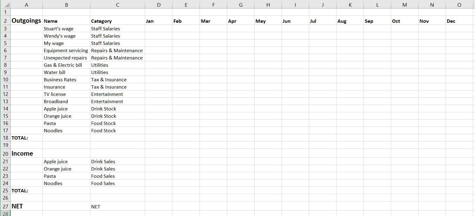
This details outgoings such as staff salaries, repair costs, utility bills and food/drink stock, as well as listing income such as food/drink sales.

Next, we can start entering financial values for each budget item and month. These figures may be based on previous accounts you’ve kept or they may be based on your best guess and available information. Now that you’ve entered those figures, it is best to format them so they are presented as currency. 

To do this, simply highlight all the Cells you’ll be using to store or calculate financial values and then right-click. A menu of options will appear and here you need to select ‘Format Cells’. Another set of options will then appear and in here you just need to select ‘Currency’. If the ‘Symbol’ is not set to the currency you need, you can click on it and choose from a list of different currencies. Finally if you want to display negative numbers differently, there are a few options available.

Once you’re happy with your selections, click OK and the numeric values in the Cells you highlighted will change to present as currency, like so:

Now that you’ve entered and formatted the financial details for all your budget items, you can use the SUM Function to create a Formula that will calculate the monthly total for all your outgoings, like so:

Here you can see that instead of selecting a whole Column, the SUM is being calculated for certain Cells, and then by using the Fill Handle the Formula is repeated and used to work out the total outgoing for each month. You can then create a similar calculation to work out the total income for each month.

Finally, we can work out the Net amount for each month by writing a simple Formula to subtract the monthly outgoings total from the monthly income total, like this:

And there you have it – a simple budget using a combination of SUM and basic Formulas. You could take this further and apply what you’ve learned about SUMIF to work out which category of your budget costs the most in December and which category of your budget generates the most income in December. You could even make a Chart or Graph of your findings. Give it a try and good luck.

Back to Top

---

What’s next?

Once you fully understand these Excel basics, the next step would be to grow your Excel knowledge further by researching Pivot Tables, Data Validation and Functions like IF, SUMIFS and COUNTIFS. You can find all sorts of guides online by searching on Google or YouTube. Watch this space too, as we’re always releasing new guides on all sorts of topics to help you with your personal and professional growth.

---

Further Resources:

• Writing A Professional Development Plan – Example & Template
• Writing a Job Description: Free Template
• How to Upskill Yourself
• Microsoft Excel and Google Sheets Training for Beginners