Help about microsoft excel

Learn from live instructors

Microsoft offers live coaching to help your learn excel formulas, tip and more to save you time and to take your skills to the next level.

Get started now

Explore Excel

Find Excel templates

Bring your ideas to life and streamline your work by starting with professionally designed, fully customizable templates from Microsoft Create.

Browse templates

Analyze Data

Ask questions about your data without having to write complicated formulas. Not available in all locales.

Explore your data

Plan and track your health

Tackle your health and fitness goals, stay on track of your progress, and be your best self with help from Excel.

Get healthy

Support for Excel 2013 has ended

Learn what end of Excel 2013 support means for you and find out how you can upgrade to Microsoft 365.

Get the details

Trending topics

Microsoft Excel know-how is so expected that it hardly warrants a line on a resume anymore. But how well do you really know how to use it?

Marketing is more data-driven than ever before. At any time you could be tracking growth rates, content analysis, or marketing ROI. You may know how to plug in numbers and add up cells in a column in Excel, but that’s not going to get you far when it comes to metrics reporting.

Do you want to understand what pivot tables are? Are you ready for your first VLOOKUP? Aspiring Excel wizard, read on or jump to the section that interests you most:

What is Microsoft Excel?

Microsoft Excel is a popular spreadsheet software program for business. It’s used for data entry and management, charts and graphs, and project management. You can format, organize, visualize, and calculate data with this tool.

How to Download Microsoft Excel

It’s easy to download Microsoft Excel. First, check to make sure that your PC or Mac meets Microsoft’s system requirements. Next, sign in and install Microsoft 365.

After you sign in, follow the steps for your account and computer system to download and launch the program.

For example, say you’re working on a Mac desktop. You’ll click on Launchpad or look in your applications folder. Then, click on the Excel icon to open the application.

Microsoft Excel Spreadsheet Basics

Sometimes, Excel seems too good to be true. Need to combine data in multiple cells? Excel can do it. Need to copy formatting across an array of cells? Excel can do that, too.

Let’s start this Excel guide with the basics. Once you have these functions down, you’ll be ready to tackle more pro Excel tips and advanced lessons.

Inserting Rows or Columns

As you work with data, you might find yourself needing to add more rows and columns. Doing this one at a time would be super tedious. Luckily, there’s an easier way.

To add multiple rows or columns in a spreadsheet, highlight the number of pre-existing rows or columns that you want to add. Then, right-click and select «Insert.»

In this example, I add three rows to the top of my spreadsheet.

Autofill

Autofill lets you quickly fill adjacent cells with several types of data, including values, series, and formulas.

There are many ways to deploy this feature, but the fill handle is among the easiest.

First, choose the cells you want to be the source. Next, find the fill handle in the lower-right corner of the cell. Then either drag the fill handle to cover the cells you want to fill or just double-click.

Filters

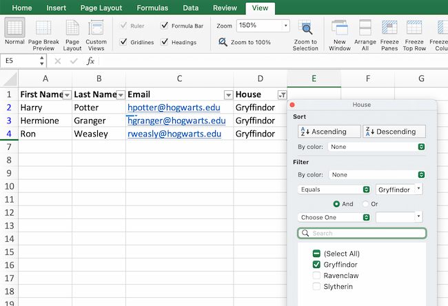
When you’re looking at large data sets, you usually don’t need to look at every row at the same time. Sometimes, you only want to look at data that fit into certain criteria. That’s where filters come in.

Filters allow you to pare down data to only see certain rows at one time. In Excel, you can add a filter to each column in your data. From there, you can choose which cells you want to view.

To add a filter, click the Data tab and select «Filter.» Next, click the arrow next to the column headers. This lets you choose whether you want to organize your data in ascending or descending order, as well as which rows you want to show.

Let’s take a look at the Harry Potter example below. Say you only want to see the students in Gryffindor. By selecting the Gryffindor filter, the other rows disappear.

Pro tip: Start with a filtered view in your original spreadsheet. Then, copy and paste the values to another spreadsheet before you start analyzing.

Sort

Sometimes you’ll have a disorganized list of data. This is typical when you’re exporting lists, like marketing contacts or blog posts. Excel’s sort feature can help you alphabetize any list.

Click on the data in the column you want to sort. Then click on the «Data» tab in your toolbar and look for the «Sort» option on the left.

• If the «A» is on top of the «Z,» you can just click on that button once. Choosing A-Z means the list will sort in alphabetical order.
• If the «Z» is on top of the «A,» click the button twice. Z-A selection means the list will sort in reverse alphabetical order.

Remove Duplicates

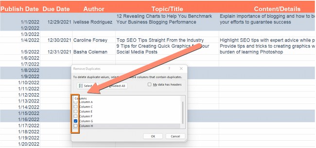
Large datasets tend to have duplicate content. For example, you may have a list of different company contacts, but you only want to see the number of companies you have. In situations like this, removing duplicates comes in handy.

To remove duplicates, highlight the row or column where you noticed duplicate data. Then, go to the Data tab, and select «Remove Duplicates» (under Tools). A pop-up will appear so that you can confirm which data you want to keep. Select «Remove Duplicates,» and you’re good to go.

If you want to see an example, this post offers step-by-step instructions for removing duplicates.

You can also use this feature to remove an entire row based on a duplicate column value. So, say you have three rows of information and you only need to see one, you can select the whole dataset and then remove duplicates. The resulting list will have only unique data without any duplicates.

Paste Special

It’s often helpful to change the items in a row of data into a column (or vice versa). It would take a lot of time to copy and paste each individual header.

Not to mention, you may easily fall into one of the biggest, most unfortunate Excel traps — human error. Read here to check out some of the most common Microsoft Excel errors.

Instead of making one of these errors, let Excel do the work for you. Take a look at this example:

To use this function, highlight the column or row you want to transpose. Then, right-click and select «Copy.»

Next, select the cells where you want the first row or column to begin. Right-click on the cell, and then select «Paste Special.»

When the module appears, choose the option to transpose.

Paste Special is a super useful function. In the module, you can also choose between copying formulas, values, formats, or even column widths. This is especially helpful when it comes to copying the results of your pivot table into a chart.

Text to Columns

What if you want to split out information that’s in one cell into two different cells? For example, maybe you want to pull out someone’s company name through their email address. Or you want to separate someone’s full name into a first and last name for your email marketing templates.

Thanks to Microsoft Excel, both are possible. First, highlight the column where you want to split up. Next, go to the Data tab and select «Text to Columns.» A module will appear with more information. First, you need to select either «Delimited» or «Fixed Width.»

• Delimited means you want to break up the column based on characters such as commas, spaces, or tabs.
• Fixed Width means you want to select the exact location in all the columns where you want the split to occur.

Select «Delimited» to separate the full name into first name and last name.

Then, it’s time to choose the delimiters. This could be a tab, semicolon, comma, space, or something else. (For example, «something else» could be the «@» sign used in an email address.) Let’s choose the space for this example. Excel will then show you a preview of what your new columns will look like.

When you’re happy with the preview, press «Next.» This page will allow you to select Advanced Formats if you choose to. When you’re done, click «Finish.»

Format Painter

Excel has a lot of features to make crunching numbers and analyzing your data quick and easy. But if you ever spent some time formatting a spreadsheet, you know it can get a bit tedious.

Don’t waste time repeating the same formatting commands over and over again. Use the format painter to copy formatting from one area of the worksheet to another.

To do this, choose the cell you’d like to replicate. Then, select the format painter option (paintbrush icon) from the top toolbar. When you release the mouse, your cell should show the new format.

Keyboard Shortcuts

Creating reports in Excel is time-consuming enough. How can we spend less time navigating, formatting, and selecting items in our spreadsheet? Glad you asked. There are a ton of Excel shortcuts out there, including some of our favorites listed below.

Create a New Workbook

PC: Ctrl-N | Mac: Command-N

Select Entire Row

PC: Shift-Space | Mac: Shift-Space

Select Entire Column

PC: Ctrl-Space | Mac: Control-Space

Select Rest of Column

PC: Ctrl-Shift-Down/Up | Mac: Command-Shift-Down/Up

Select Rest of Row

PC: Ctrl-Shift-Right/Left | Mac: Command-Shift-Right/Left

Add Hyperlink

PC: Ctrl-K | Mac: Command-K

Open Format Cells Window

PC: Ctrl-1 | Mac: Command-1

Autosum Selected Cells

PC: Alt-= | Mac: Command-Shift-T

Excel Formulas

At this point, you’re getting used to Excel’s interface and flying through quick commands on your spreadsheets.

Now, let’s dig into the core use case for the software: Excel formulas. Excel can help you do simple arithmetic like adding, subtracting, multiplying, or dividing any data.

• To add, use the + sign.
• To subtract, use the — sign.
• To multiply, use the * sign.
• To divide, use the / sign.
• To use exponents, use the ^ sign.

Remember, all formulas in Excel must begin with an equal sign (=). Use parentheses to make sure certain calculations happen first. For example, consider how =10+10*10 is different from =(10+10)*10.

Besides manually typing in simple calculations, you can also refer to Excel’s built-in formulas. Some of the most common include:

• Average: =AVERAGE(cell range)
• Sum: =SUM(cell range)
• Count: =COUNT(cell range)

Also note that series’ of specific cells are separated by a comma (,), while cell ranges are notated with a colon (:). For example, you could use any of these formulas:

• =SUM(4,4)
• =SUM(A4,B4)
• =SUM(A4:B4)

Conditional Formatting

Conditional formatting lets you change a cell’s color based on the information within the cell. For example, say you want to flag a category in your spreadsheet.

To get started, highlight the group of cells you want to use conditional formatting on. Then, choose «Conditional Formatting» from the Home menu. Next, select a logic option from the dropdown. A window will pop up that prompts you to provide more information about your formatting rule. Select «OK» when you’re done, and you should see your results automatically appear.

Note: You can also create your own logic if you want something beyond the dropdown choices.

Dollar Signs

Have you ever seen a dollar sign in an Excel formula? When this symbol is in a formula, it isn’t representing an American dollar. Instead, it makes sure that the exact column and row stay the same even if you copy the same formula in adjacent rows.

You see, a cell reference — when you refer to cell A5 from cell C5, for example — is relative by default.

This means you’re actually referring to a cell that’s five columns to the left (C minus A) and in the same row (5). This is called a relative formula.

When you copy a relative formula from one cell to another, it’ll adjust the values in the formula based on where it’s moved. But sometimes, you want those values to stay the same no matter whether they’re moved around or not. You can do that by making the formula in the cell into what’s called an absolute formula.

To change the relative formula (=A5+C5) into an absolute formula, precede the row and column values with dollar signs, like this: (=$A$5+$C$5).

Combine Cells Using «&»

Databases tend to split out data to make it as exact as possible. For example, instead of having data that shows a person’s full name, a database might have the data as a first name and then a last name in separate columns.

In Excel, you can combine cells with different data into one cell by using the «&» sign in your function. The example below uses this formula: =A2&» «&B2.

Let’s go through the formula together using an example. So, let’s combine first names and last names into full names in a single column.

To do this, put your cursor in the blank cell where you want the full name to appear. Next, highlight one cell that contains a first name, type in an «&» sign, and then highlight a cell with the corresponding last name.

But you’re not finished. If all you type in is =A2&B2, then there will not be a space between the person’s first name and last name. To add that necessary space, use the function =A2&» «&B2. The quotation marks around the space tell Excel to put a space between the first and last name.

To make this true for multiple rows, drag the corner of that first cell downward as shown in the example.

Pivot Tables

Pivot tables reorganize data in a spreadsheet. A pivot table won’t change the data that you have, but it can sum up values and compare information in a way that’s easy to understand.

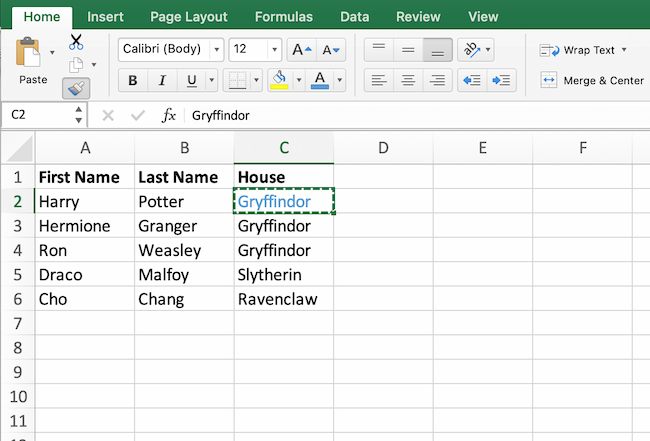
For example, let’s look at how many people are in each house at Hogwarts.

To create the Pivot Table, go to Insert > Pivot Table. Excel will automatically populate your pivot table, but you can always change the order of the data. Then, you have four options to choose from.

Report Filter

This allows you to only look at certain rows in your dataset.

For example, to create a filter by house, choose only students in Gryffindor.

Column and Row Labels

These could be any headers or rows in the dataset.

Note: Both Row and Column labels can contain data from your columns. For example, you can drag First Name to either the Row or Column label depending on how you want to see the data.

Value

This section allows you to convert data into a number. Instead of just pulling in any numeric value, you can sum, count, average, max, min, count numbers, or do a few other manipulations with your data. By default, when you drag a field to Value, it always does a count.

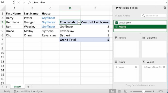
The example above counts the number of students in each house. To recreate this pivot table, go to the pivot table and drag the House column to both the row Labels and the values. This will sum up the number of students associated with each house.

IF Functions

At its most basic level, Excel’s IF function lets you see if a condition you set is true or false for a given value.

If the condition is true, you get one result. If the condition is false, you get another result.

This popular tool is useful for comparisons and finding errors. But if you’re new to Excel you may need a little more information to get the most out of this feature.

Let’s take a look at this function’s syntax:

• =IF(logical_test, value_if_true, [value_if_false])

• With values, this could be: =IF(A2>B2, «Over Budget», «OK»)

In this example, you want to find where you’re overspending. With this IF function, if your spending (what’s in A2) is greater than your budget (what’s in B2), that overspending will be easy to see. Then you can then filter the data so that you see only the line items where you’re going over budget.

The real power of the IF function comes when you string or «nest» multiple IF statements together. This allows you to set multiple conditions, get more specific results, and organize your data into more manageable chunks.

For example, ranges are one way to segment your data for better analysis. For example, you can categorize data into values that are less than 10, 11 to 50, or 51 to 100.

• =IF(B3<11,»10 or less»,IF(B3<51,»11 to 50″,IF(B3<100,»51 to 100″)))

Let’s talk about a few more IF functions.

COUNTIF Function

The power of IF functions goes beyond simple true and false statements. With the COUNTIF function, Excel can count the number of times a word or number appears in any range of cells.

For example, let’s say you want to count the number of times the word «Gryffindor» appears in this data set.

Take a look at the syntax.

• The formula: =COUNTIF(range, criteria)
• The formula with variables from the example below: =COUNTIF(D:D,»Gryffindor»)

In this formula, there are several variables:

Range

The range that you want the formula to cover.

In this one-column example, «D:D» shows that the first and last columns are both D. If you want to look at columns C and D, use «C:D.»

Criteria

Whatever number or piece of text you want Excel to count.

Only use quotation marks if you want the result to be text instead of a number. In this example, «Gryffindor» is the only criteria.

To use this function, type the COUNTIF formula in any cell and press «Enter.» Using the example above, this action will show how many times the word «Gryffindor» appears in the dataset.

SUMIF Function

Ready to make the IF function a bit more complex? Let’s say you want to analyze the number of leads your blog has generated from one author, not the entire team.

With the SUMIFS function, you can add up cells that meet certain criteria. You can add as many different criteria to the formula as you like.

Here’s your formula:

• =SUMIFS(sum_range, criteria_range1, criteria1, [criteria_range2, criteria 2],etc.)

That’s a lot of criteria. Let’s take a look at each part:

Sum_range

The range of cells you’re going to add up.

Criteria_range1

The range that is being searched for your first value.

Criteria1

This is the specific value that determines which cells in Criteria_range1 to add together.

Note: Remember to use quotation marks if you’re searching for text.

In the example below, the SUMIF formula counts the total number of house points from Gryffindor.

If AND/OR

The OR and AND functions round out your IF function choices. These functions check multiple arguments. It returns either TRUE or FALSE depending on if at least one of the arguments is true (this is the OR function), or if all of them are true (this is the AND function).

Lost in a sea of «and’s» and «or’s»? Don’t check out yet. In practice, OR and AND functions will never be used on their own. They need to be nested inside of another IF function. Recall the syntax of a basic IF function:

• =IF(logical_test, value_if_true, [value_if_false])
• Now, let’s fit an OR function inside of the logical_test: =IF(OR(logical1, logical2), value_if_true, [value_if_false])

To put it plainly, this combined formula allows you to return a value if both conditions are true, as opposed to just one. With AND/OR functions, your formulas can be as simple or complex as you want them to be, as long as you understand the basics of the IF function.

VLOOKUP

Have you ever had two sets of data on two different spreadsheets that you want to combine into a single spreadsheet?

For example, say you have a list of names and email addresses in one spreadsheet and a list of email addresses and company names in a different spreadsheet. But you want the names, email addresses, and company names of those people to appear in one spreadsheet.

VLOOKUP is a great go-to formula for this.

Before you use the formula, be sure that you have at least one column that appears identically in both places.

Note: Scour your data sets to make sure the column of data you’re using to combine spreadsheets is exactly the same. This includes removing any extra spaces.

In the example below, Sheet One and Sheet Two are both lists with different information about the same people. The common thread between the two is their email addresses. Let’s combine both datasets so that all the house information from Sheet Two translates over to Sheet One.

Type in the formula: =VLOOKUP(C2,Sheet2!A:B,2,FALSE). This will bring all the house data into Sheet One.

Now that you’ve seen how VLOOKUP works, let’s review the formula.

• The formula: =VLOOKUP(lookup value, table array, column number, [range lookup])
• The formula with variables from the example: =VLOOKUP(C2,Sheet2!A:B,2,FALSE)

In this formula, there are several variables.

Lookup Value

A value that LOOKUP searches for in an array. So, your lookup value is the identical value you have in both spreadsheets.

In the example, the lookup value is the first email address on the list, or cell 2 (C2).

Table Array

Table arrays hold column-oriented or tabular data, like the columns on Sheet Two you’re going to pull your data from.

This table array includes the column of data identical to your lookup value in Sheet One and the column of data you’re trying to copy to Sheet Two.

In the example, «A» means Column A in Sheet Two. The «B» means Column B.

So, the table array is «Sheet2!A:B.»

Column Number

Excel refers to columns as letters and rows as numbers. So, the column number is the selected column for the new data you want to copy.

In the example, this would be the «House» column. «House» is column 2 in the table array.

Note: Your range can be more than two columns. For example, if there are three columns on Sheet Two — Email, Age, and House — and you also want to bring House onto Sheet One, you can still use a VLOOKUP. You just need to change the «2» to a «3» so it pulls back the value in the third column. The formula for this would be: =VLOOKUP(C2:Sheet2!A:C,3,false).]

Range Lookup

This term means that you’re looking for a value within a range of values. You can also use the term «FALSE» to pull only exact value matches.

Note: VLOOKUP will only pull back values to the right of the column containing your identical data on the second sheet. This is why some people prefer to use the INDEX and MATCH functions instead.

INDEX MATCH

Like VLOOKUP, the INDEX and MATCH functions pull data from another dataset into one central location. Here are the main differences:

VLOOKUP is a much simpler formula.

If you’re working with large datasets that need thousands of lookups, the INDEX MATCH function will decrease load time in Excel.

INDEX MATCH formulas work right-to-left.

VLOOKUP formulas only work as a left-to-right lookup. So, if you need to do a lookup that has a column to the right of the results column, you’d have to rearrange those columns to do a VLOOKUP. This can be tedious with large datasets and lead to errors.

Let’s look at an example. Let’s say Sheet One contains a list of names and their Hogwarts email addresses. Sheet Two contains a list of email addresses and each student’s Patronus.

The information that lives in both sheets is the email addresses column. But, the column numbers for email addresses are different on the two sheets. So, you’d use the INDEX MATCH formula instead of VLOOKUP to avoid column-switching errors.

The INDEX MATCH formula is the MATCH formula nested inside the INDEX formula.

• The formula: =INDEX(table array, MATCH formula)
• This becomes: =INDEX(table array, MATCH (lookup_value, lookup_array))
• The formula with variables from the example: =INDEX(Sheet2!A:A,(MATCH(Sheet1!C:C,Sheet2!C:C,0)))

Here are the variables:

Table Array

The range of columns on Sheet Two that contain the new data you want to bring over to Sheet One.

In the example, «A» means Column A, and has the «Patronus» information for each person.

Lookup Value

This Sheet One column has identical values in both spreadsheets.

In the example, this is the «email» column on Sheet One, which is Column C. So, Sheet1!C:C.

Lookup Array

Again, an array is a group of values in rows and columns that you want to search.

In this example, the lookup array is the column in Sheet Two that contains identical values in both spreadsheets. So, the «email» column on Sheet Two, Sheet2!C:C.

Once you have your variables set, type in the INDEX MATCH formula. Add it where you want the combined information to populate.

Data Visualization

Now that you’ve learned formulas and functions, let’s make your analysis visual. With a beautiful graph, your audience will be able to process and remember your data more easily.

Create a Basic Graph

First, decide what type of graph to use. Bar charts and pie charts help you compare categories. Pie charts compare part of a whole and are often best when one of the categories is way larger than the others. Bar charts highlight incremental differences between categories. Finally, line charts can help display trends over time.

This post can help you find the best chart or graph for your presentation.

Next, highlight the data you want to turn into a chart. Then choose «Charts» in the top navigation. You can also use Insert > Chart if you have an older version of Excel. Then you can adjust and resize your chart until it makes the statement you’re hoping for.

Microsoft Excel Can Help Your Business Grow

Excel is a useful tool for any small business. Whether you’re focused on marketing, HR, sales, or service, these Microsoft Excel tips can boost your performance.

Whether you want to improve efficiency or productivity, Excel can help. You can find new trends and organize your data into usable insights. It can make your data analysis easier to understand and your daily tasks easier.

All it takes is a little know-how and some time with the software. So start learning, and get ready to grow.

Editor’s note: This post was originally published in April 2018 and has been updated for comprehensiveness.

Microsoft Excel – самая популярная программа для работы с электронными таблицами. Ее преимущество заключается в наличии всех базовых и продвинутых функций, которые подойдут как новичкам, так и опытным пользователям, нуждающимся в профессиональном ПО.

В рамках этой статьи я хочу рассказать о том, как начать работу в Эксель и понять принцип взаимодействия с данным софтом.

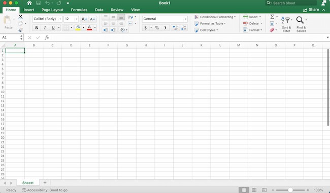
Создание таблицы в Microsoft Excel

Конечно, в первую очередь необходимо затронуть тему создания таблиц в Microsoft Excel, поскольку эти объекты являются основными и вокруг них строится остальная работа с функциями. Запустите программу и создайте пустой лист, если еще не сделали этого ранее. На экране вы видите начерченный проект со столбцами и строками. Столбцы имеют буквенное обозначение, а строки – цифренное. Ячейки образовываются из их сочетания, то есть A1 – это ячейка, располагающаяся под первым номером в столбце группы А. С пониманием этого не должно возникнуть никаких проблем.

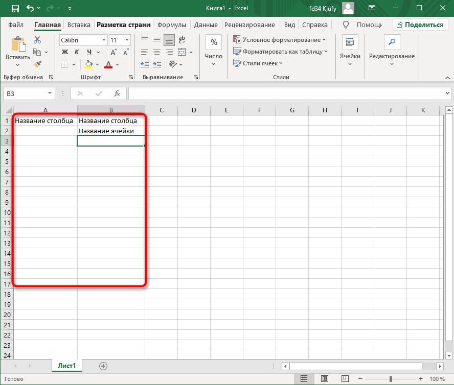
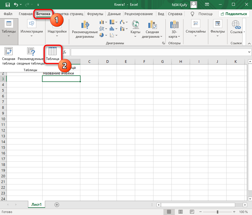
Обратите внимание на приведенный выше скриншот. Вы можете задавать любые названия для столбцов, заполняя данные в ячейках. Именно так формируется таблица. Если не ставить для нее границ, то она будет бесконечной. В случае необходимости создания выделенной таблицы, которую в будущем можно будет редактировать, копировать и связывать с другими листами, перейдите на вкладку «‎Вставка» и выберите вариант вставки таблицы.

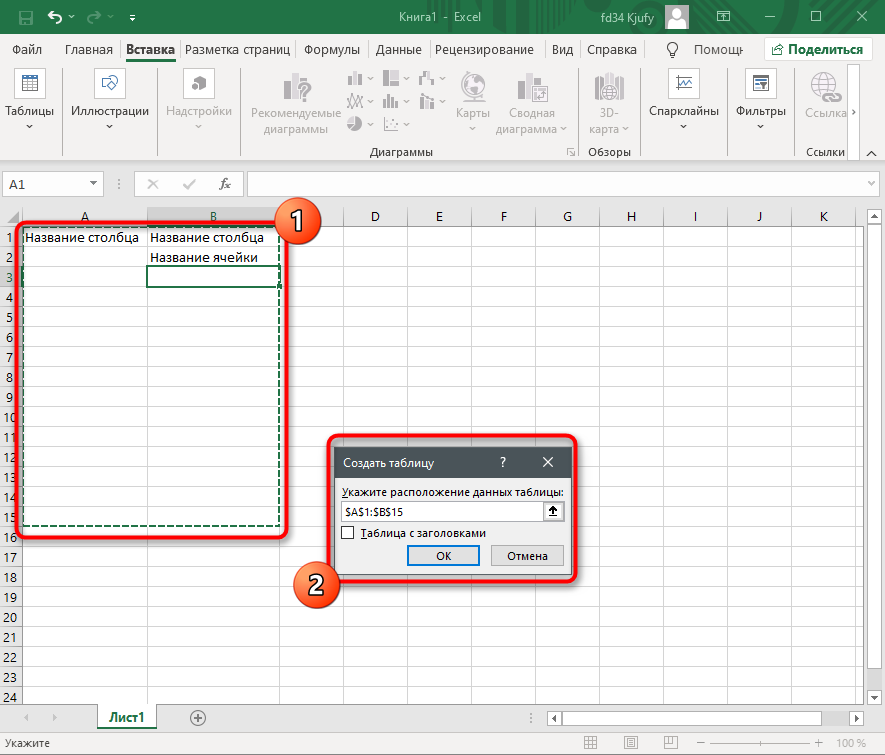
Задайте для нее необходимую область, зажав левую кнопку мыши и потянув курсор на необходимое расстояние, следя за тем, какие ячейки попадают в пунктирную линию. Если вы уже разобрались с названиями ячеек, можете заполнить данные самостоятельно в поле расположения. Однако там нужно вписывать дополнительные символы, с чем новички часто незнакомы, поэтому проще пойти предложенным способом. Нажмите «‎ОК» для завершения создания таблицы.

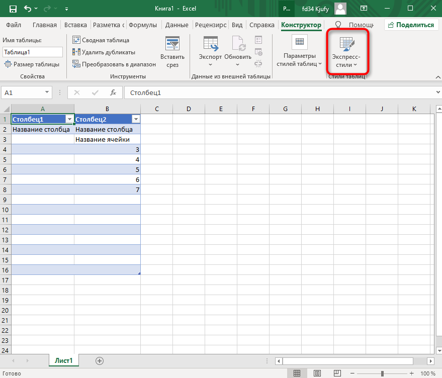
На листе вы сразу же увидите сформированную таблицу с группировками по столбцам, которые можно сворачивать, если их отображение в текущий момент не требуется. Видно, что таблица имеет свое оформление и точно заданные границы. В будущем вам может потребоваться увеличение или сокращение таблицы, поэтому вы можете редактировать ее параметры на вкладке «‎Конструктор».

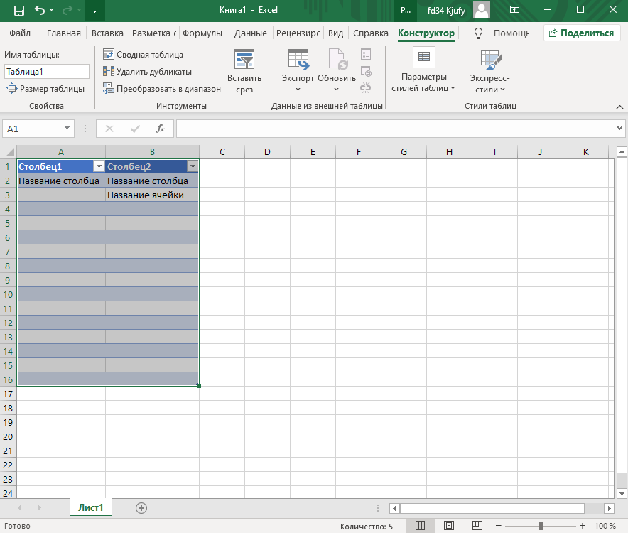
Обратите внимание на функцию «‎Экспресс-стили», которая находится на той же упомянутой вкладке. Она предназначена для изменения внешнего вида таблицы, цветовой гаммы. Раскройте список доступных тем и выберите одну из них либо приступите к созданию своей, разобраться с чем будет не так сложно.

Основные элементы редактирования

Работать в Excel самостоятельно – значит, использовать встроенные элементы редактирования, которые обязательно пригодятся при составлении таблиц. Подробно останавливаться на них мы не будем, поскольку большинство из предложенных инструментов знакомы любому пользователю, кто хотя бы раз сталкивался с подобными элементами в том же текстовом редакторе от Microsoft. 

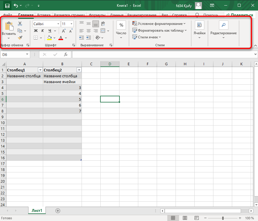
На вкладке «‎Главная» вы увидите все упомянутые инструменты. С их помощью вы можете управлять буфером обмена, изменять шрифт и его формат, использовать выравнивание текста, убирать лишние знаки после запятой в цифрах, применять стили ячеек и сортировать данные через раздел «‎Редактирование».

Использование функций Excel

По сути, создать ту же таблицу можно практически в любом текстовом или графическом редакторе, но такие решения пользователям не подходят из-за отсутствия средств автоматизации. Поэтому большинство пользователей, которые задаются вопросом «‎Как научиться работать в Excel», желают максимально упростить этот процесс и по максимуму задействовать все встроенные инструменты. Главные средства автоматизации – функции, о которых и пойдет речь далее.

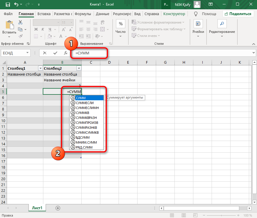
1. Если вы желаете объявить любую функцию в ячейке (результат обязательно выводится в поле), начните написание со знака «​=», после чего впишите первый символ, обозначающий название формулы. На экране появится список подходящих вариантов, а нажатие клавиши TAB выбирает одну из них и автоматически дописывает оставшиеся символы.

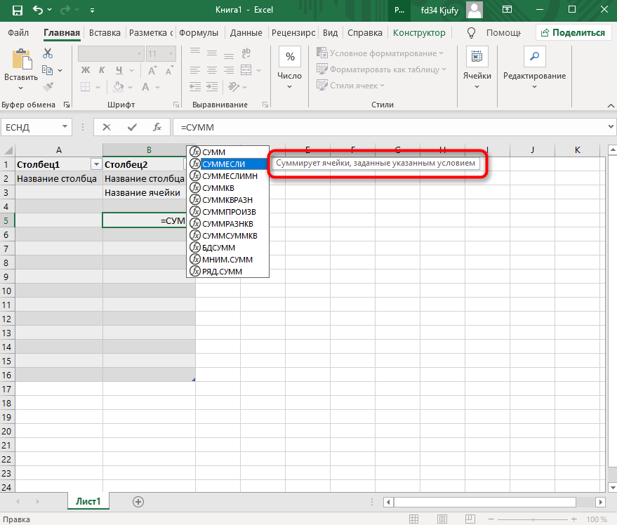
2. Обратите внимание на то, что справа от имени выбранной функции показывается ее краткое описание от разработчиков, позволяющее понять предназначение и действие, которое она выполняет.

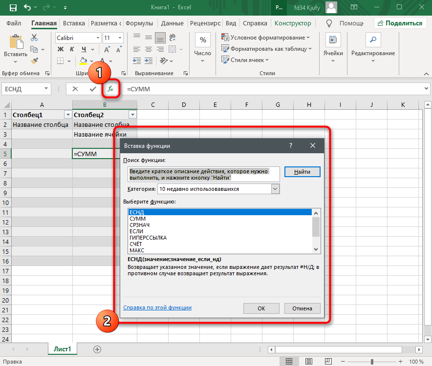
3. Если кликнуть по значку с функцией справа от поля ввода, на экране появится специальное окно «‎Вставка функции», в котором вы можете ознакомиться со всеми ними еще более детально, получив полный список и справку. Если выбрать одну из функций, появится следующее окно редактирования, где указываются аргументы и опции. Это позволит не запутаться в правильном написании значений.

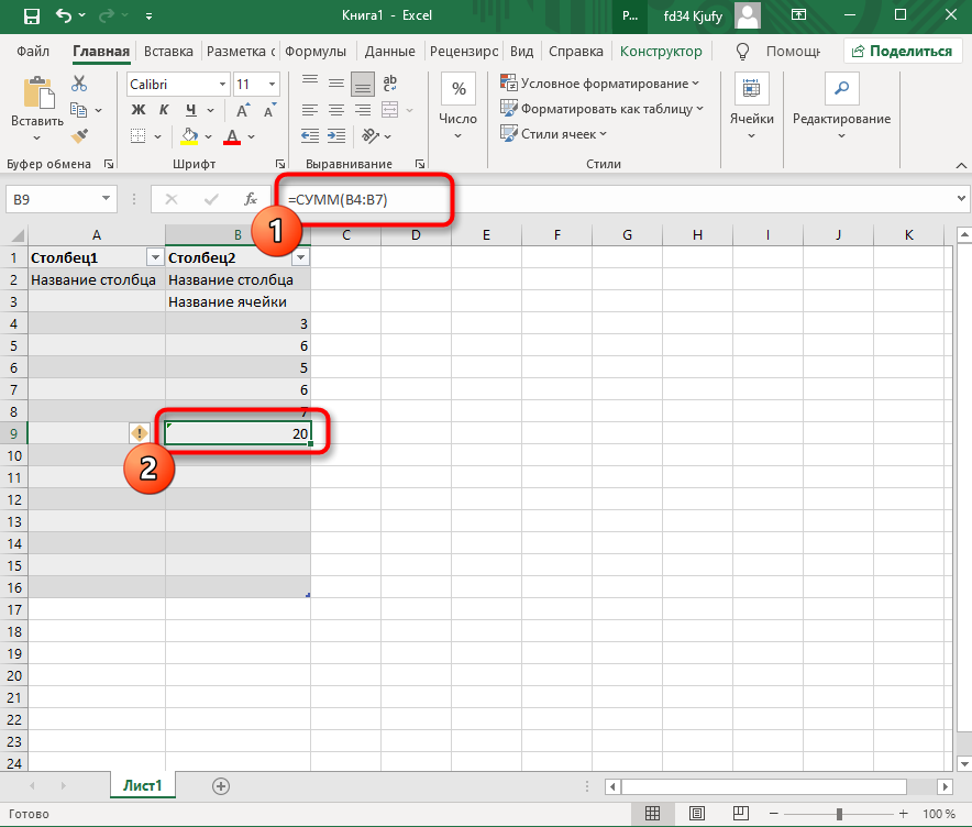
4. Взгляните на следующее изображение. Это пример самой простой функции, результатом которой является сумма указанного диапазона ячеек или двух из них. В данном случае знак «:»​ означает, что все значения ячеек указанного диапазона попадают под выражение и будут суммироваться. Все формулы разобрать в одной статье нереально, поэтому читайте официальную справку по каждой или найдите открытую информацию в сети.

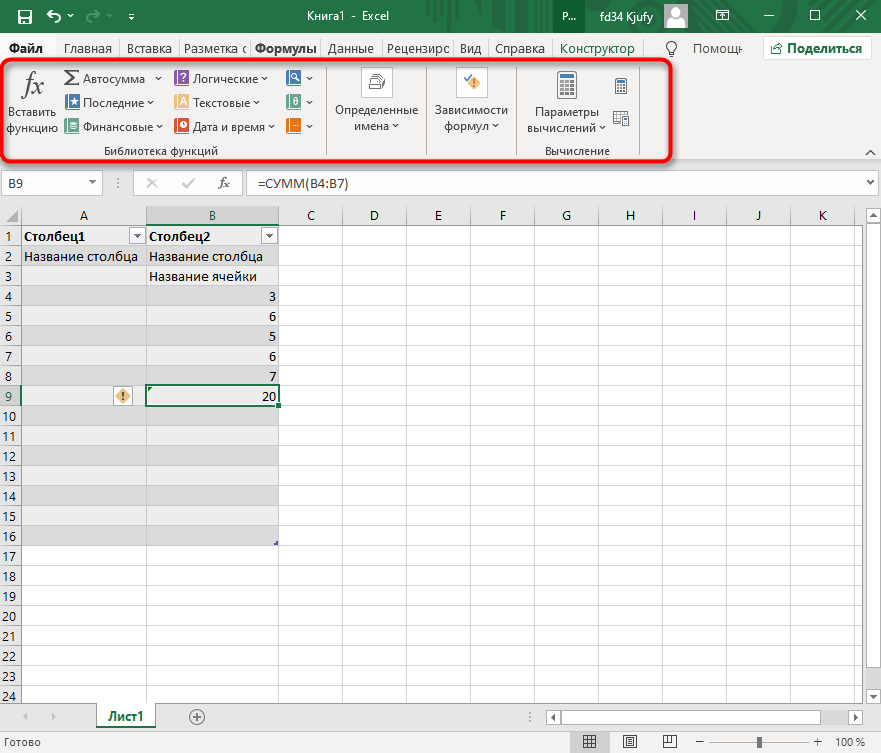
5. На вкладке с формулами вы можете найти любую из них по группам, редактировать параметры вычислений или зависимости. В большинстве случаев это пригождается только опытным пользователям, поэтому просто упомяну наличие такой вкладки с полезными инструментами.

Вставка диаграмм

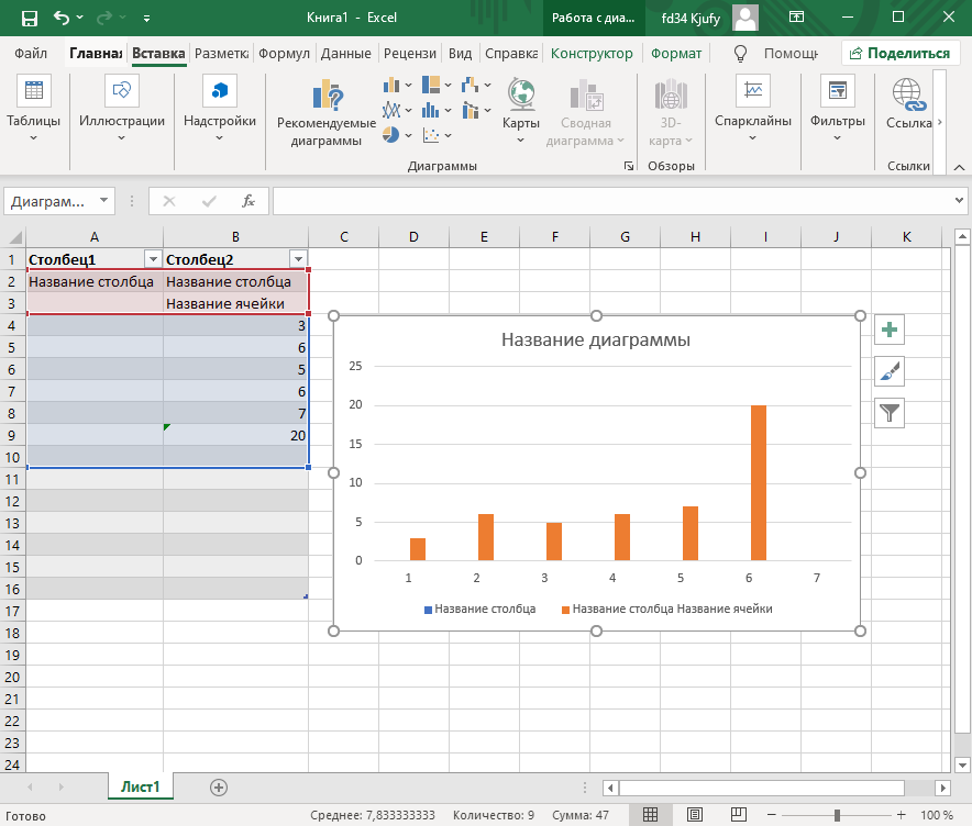
Часто работа в Эксель подразумевает использование диаграмм, зависимых от составленной таблицы. Обычно это требуется ученикам, которые готовят на занятия конкретные проекты с вычислениями, однако применяются графики и в профессиональных сферах. На данном сайте есть другая моя инструкция, посвященная именно составлению диаграммы по таблице. Она поможет разобраться во всех тонкостях этого дела и самостоятельно составить график необходимого типа.

Подробнее: Как построить диаграмму по таблице в Excel: пошаговая инструкция

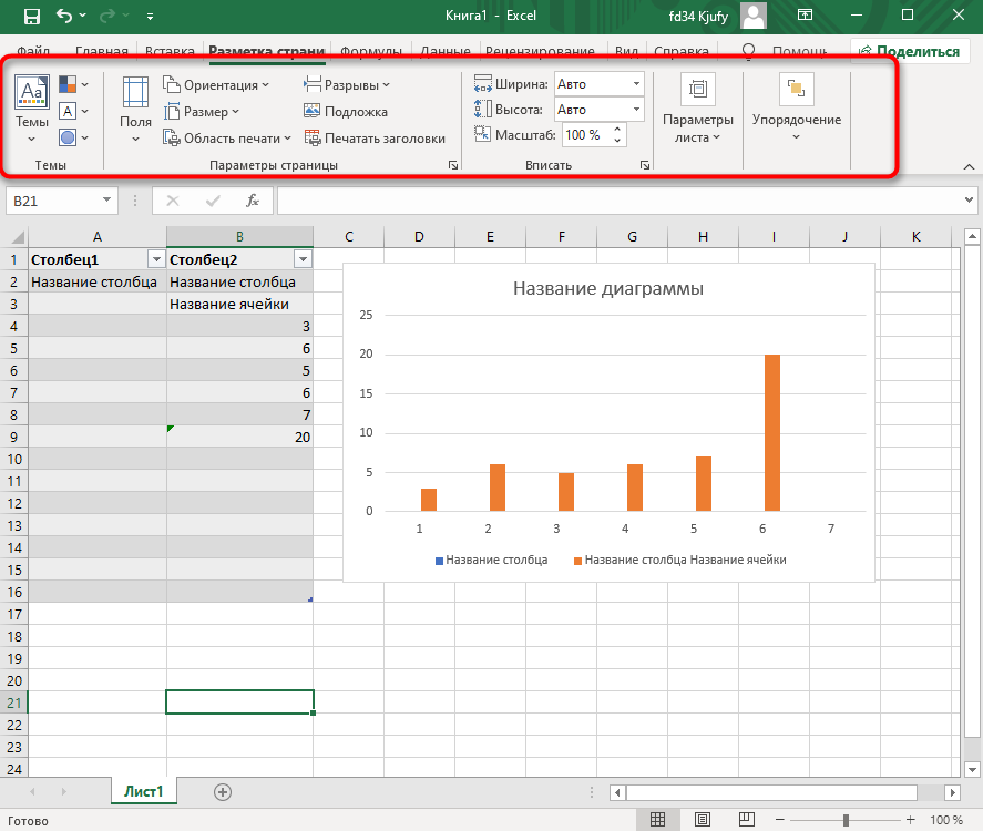
Элементы разметки страницы

Вкладка под названием «‎Разметка страницы» пригодится вам только в том случае, если создаваемый лист в будущем должен отправиться в печать. Здесь вы найдете параметры страницы, сможете изменить ее размер, ориентацию, указать область печати и выполнить другое редактирование. Большинство доступных инструментов подписаны, и с их использованием не возникнет никаких проблем. Учитывайте, что при внесении изменений вы можете нажать комбинацию клавиш Ctrl + Z, если вдруг что-то сделали не так.

Сохранение и переключение между таблицами

Программа Эксель подразумевает огромное количество мелочей, на разбор которых уйдет ни один час времени, однако начинающим пользователям, желающим разобраться в базовых вещах, представленной выше информации будет достаточно. В завершение отмечу, что на главном экране вы можете сохранять текущий документ, переключаться между таблицами, отправлять их в печать или использовать встроенные шаблоны, когда необходимо начать работу с заготовками.

Надеюсь, что эта статья помогла разобраться вам с тем, как работать в Excel хотя бы на начальном уровне. Не беспокойтесь, если что-то не получается с первого раза. Воспользуйтесь поисковиком, введя там запрос по теме, ведь теперь, когда имеются хотя бы общие представления об электронных таблицах, разобраться в более сложных вопросах будет куда проще.