Headers in excel sheet - Word и Excel - помощь в работе с программами

Excel for Microsoft 365 Excel 2021 Excel 2019 Excel 2016 Excel 2013 Excel 2010 Excel 2007 Excel Starter 2010 More…Less

You can add headers or footers at the top or bottom of a printed worksheet in Excel. For example, you might create a footer that has page numbers, the date, and the name of your file. You can create your own, or use many built-in headers and footers.

Headers and footers are displayed only in Page Layout view, Print Preview, and on printed pages. You can also use the Page Setup dialog box if you want to insert headers or footers for more than one worksheet at a time. For other sheet types, such as chart sheets, or charts, you can insert headers and footers only by using the Page Setup dialog box.

Add or change headers or footers in Page Layout view

Click the worksheet where you want to add or change headers or footers.
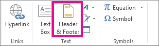
On the Insert tab, in the Text group, click Header & Footer.

Excel displays the worksheet in Page Layout view.
To add or edit a header or footer, click the left, center, or right header or footer text box at the top or the bottom of the worksheet page (under Header, or above Footer).
Type the new header or footer text.
Notes:
- To start a new line in a header or footer text box, press Enter.
- To include a single ampersand (&) in the text of a header or footer, use two ampersands. For example, to include «Subcontractors & Services» in a header, type Subcontractors && Services.
- To close headers or footers, click anywhere in the worksheet. To close headers or footers without keeping the changes that you made, press Esc.

Click the worksheet or worksheets, chart sheet, or chart where you want to add or change headers or footers.

Tip: You can select multiple worksheets with Ctrl+Left-click. When multiple worksheets are selected, [Group] appears in the title bar at the top of the worksheet. To cancel a selection of multiple worksheets in a workbook, click any unselected worksheet. If no unselected sheet is visible, right-click the tab of a selected sheet, and then click Ungroup Sheets.
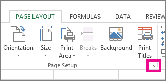
On the Page Layout tab, in the Page Setup group, click the Dialog Box Launcher .

Excel displays the Page Setup dialog box.
On the Header/Footer tab, click Custom Header or Custom Footer.
Click in the Left, Center, or Right section box, and then click any of the buttons to add the header or footer information that you want in that section.
To add or change the header or footer text, type additional text or edit the existing text in the Left, Center, or Right section box.
Notes:
- To start a new line in a header or footer text box, press Enter.
- To include a single ampersand (&) in the text of a header or footer, use two ampersands. For example, to include «Subcontractors & Services» in a header, type Subcontractors && Services.

Excel has many built-in text headers and footers that you can use. For worksheets, you can work with headers and footers in Page Layout view. For chart sheets or charts you need to go through the Page Setup dialog.

Click the worksheet where you want to add or change a built-in header or footer.
On the Insert tab, in the Text group, click Header & Footer.

Excel displays the worksheet in Page Layout view.
Click the left, center, or right header or the footer text box at the top or the bottom of the worksheet page.

Tip: Clicking any text box selects the header or footer and displays the Header and Footer Tools, adding the Design tab.
On the Design tab, in the Header & Footer group, click Header or Footer, and then click the built-in header or footer that you want.

Instead of picking a built-in header or footer, you can choose a built-in element. Many elements (such as Page Number, File Name, and Current Date) are found on the ribbon. For worksheets, you can work with headers and footers in Page Layout view. For chart sheets or charts, you can work with headers and footers in the Page Setup dialog.

Click the worksheet to which you want to add specific header or footer elements.
On the Insert tab, in the Text group, click Header & Footer.

Excel displays the worksheet in Page Layout view.
Click the left, center, or right header or footer text box at the top or the bottom of the worksheet page.

Tip: Clicking any text box selects the header or footer and displays the Header and Footer Tools, adding the Design tab.
On the Design tab, in the Header & Footer Elements group, click the elements that you want.

Click the chart sheet or chart where you want to add or change a header or footer element.
On the Insert tab, in the Text group, click Header & Footer.

Excel displays the Page Setup dialog box.
Click Custom Header or Custom Footer.
Use the buttons in the Header or Footer dialog box to insert specific header and footer elements.

Tip: When you rest the mouse pointer on a button, a ScreenTip displays the name of the element that the button inserts.

For worksheets, you can work with headers and footers in Page Layout view. For chart sheets or charts, you can work with headers and footers in the Page Setup dialog.

Click the worksheet where you want to choose header and footer options.
On the Insert tab, in the Text group, click Header & Footer.

Excel displays the worksheet in Page Layout view.
Click the left, center, or right header or footer text box at the top or the bottom of the worksheet page.

Tip: Clicking any text box selects the header or footer and displays the Header and Footer Tools, adding the Design tab.
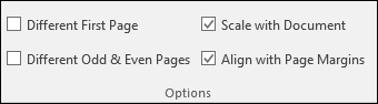
On the Design tab, in the Options group, check one or more of the following:
- To remove headers and footers from the first printed page, select the Different First Page check box.
- To specify that the headers and footers on odd-numbered pages should differ from those on even-numbered pages, select the Different Odd & Even Pages check box.
- To specify whether the headers and footers should use the same font size and scaling as the worksheet, select the Scale with Document check box.
  
  To make the font size and scaling of the headers or footers independent of the worksheet scaling, which helps create a consistent display across multiple pages, clear this check box.
- To make sure the header or footer margin is aligned with the left and right margins of the worksheet, select the Align with Page Margins check box.
  
  To set the left and right margins of the headers and footers to a specific value that is independent of the left and right margins of the worksheet, clear this check box.

Click the chart sheet or chart where you want to choose header or footer options.
On the Insert tab, in the Text group, click Header & Footer.

Excel displays the Page Setup dialog box.
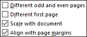
Select one or more of the following:
- To remove headers and footers from the first printed page, select the Different first page check box.
- To specify that the headers and footers on odd-numbered pages should differ from those on even-numbered pages, select the Different odd & even pages check box.
- To specify whether the headers and footers should use the same font size and scaling as the worksheet, select the Scale with document check box.
  
  To make the font size and scaling of the headers or footers independent of the worksheet scaling, which helps create a consistent display across multiple pages, clear the Scale with Document check box.
- To guarantee that the header or footer margin is aligned with the left and right margins of the worksheet, select the Align with page margins check box.
  
  Tip: To set the left and right margins of the headers and footers to a specific value that is independent of the left and right margins of the worksheet, clear this check box.

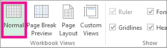
To close the header and footer, you must switch from Page Layout view to Normal view.

On the View tab, in the Workbook Views group, click Normal.

You can also click Normal on the status bar.

On the Insert tab, in the Text group, click Header & Footer.

Excel displays the worksheet in Page Layout view.
Click the left, center, or right header or the footer text box at the top or the bottom of the worksheet page.

Tip: Clicking any text box selects the header or footer and displays the Header and Footer Tools, adding the Design tab.
Press Delete or Backspace.

Note: If you want to delete headers and footers for several worksheets at once, select the worksheets, and then open the Page Setup dialog box. To delete all headers and footers instantly, on the Header/Footer tab, select (none) in the Header or Footer box.

Top of Page

Need more help?

You can always ask an expert in the Excel Tech Community or get support in the Answers community.

How do I make the first row in Excel a column header?

With a cell in your table selected, click on the “Format as Table” option in the HOME menu. When the “Format As Table” dialog comes up, select the “My table has headers” checkbox and click the OK button. Select the first row; which should be your header row.

Row header or Row heading is the gray-colored column located on the left side of column 1 in the worksheet, which contains the numbers (1, 2, 3, etc.) where it helps out to identify each row in the worksheet.

A row heading identifies a row on a worksheet. Row headings are at the left of each row and are indicated by numbers.

How do I create a column header row in Excel?

Open the Spreadsheet

Open the Spreadsheet.
Open the spreadsheet where you want to have Excel make the top row a header row.
Add a Header Row.
Enter the column headings for your data across the top row of the spreadsheet, if necessary.
Select the First Data Row.

A header in excel: It is a section of the worksheet that appears at the top of each of the pages in the excel sheet or document. This remains constant across all the pages. It can contain information such as Page No., Date, Title or Chapter Name, etc.

How do you make a title for a sheet?

How to Put a Title on Google Sheets

Open the spreadsheet.
Change the file name at the top of the window.
Click File, then Print.
Select Headers & footers.
Select Workbook title or Sheet name.
Click Next.
Click Print.

How do I freeze a row in Excel?

To freeze the top row or first column:

From the View tab, Windows Group, click the Freeze Panes drop down arrow.
Select either Freeze Top Row or Freeze First Column.
Excel inserts a thin line to show you where the frozen pane begins.

What are column headers?

In Excel and other spreadsheet applications, the column header is the colored row of letters used to identify each columnwithin the sheet, or workbook. The column header row is located above the row one.

On the status bar, click the Page Layout View button. Select the header or footer text you want to change. On the Home tab in the Font group, set the formatting options that you want to apply to the header / footer.

What is footer and header?

A header is text that is placed at the top of a page, while a footer is placed at the bottom, or foot, of a page. Typically these areas are used for inserting document information, such as the name of the document, the chapter heading, page numbers, creation date and the like.

How do you name a spreadsheet in Google Sheets?

To rename a sheet:

Click the tab of the sheet you want to rename. Select Rename… from the menu that appears.
Type the desired name for the sheet.
Click anywhere outside of the tab or press Enter on your keyboard when you’re finished, and the sheet will be renamed.

How do I change the title of a Google sheet?

Make a title or heading

On your computer, open a document in Google Docs.
Select the text you want to change.
Click Format. Paragraph styles.
Click a text style: Normal text. Title. Subtitle. Heading 1-6.
Click Apply ‘text style. ‘

Can you freeze a row and a column in Excel?

You can choose to freeze just the top row of your worksheet, just the left column of your worksheet, or multiple rows and columns simultaneously.To lock more than one row or column, or to lock both rows and columns at the same time, choose the View tab, and then click Freeze Panes.

How do you freeze 3 rows in Excel?

To freeze rows:

Select the row below the row(s) you want to freeze. In our example, we want to freeze rows 1 and 2, so we’ll select row 3.
Click the View tab on the Ribbon.
Select the Freeze Panes command, then choose Freeze Panes from the drop-down menu.
The rows will be frozen in place, as indicated by the gray line.

How do I run goal seek in Excel?

Use Goal Seek to determine the interest rate

On the Data tab, in the Data Tools group, click What-If Analysis, and then click Goal Seek.
In the Set cell box, enter the reference for the cell that contains the formula that you want to resolve.
In the To value box, type the formula result that you want.

How do I make column headers in Google Sheets?

Making custom headers in Google Sheets is very easy. All you have to do is add a blank row to the top of your document. Enter the name of each header and then freeze that row. If you’re using the Google Sheets app, you’ll see a gray line that’s now separating the column header from the rest of the cells.

How do I make the top row of Google Sheets always visible?

Freeze or unfreeze rows or columns

On your computer, open a spreadsheet in Google Sheets.
Select a row or column you want to freeze or unfreeze.
At the top, click View. Freeze.
Select how many rows or columns to freeze.

Источник

Headers and footers in Excel are inserted across multiple products of Microsoft Office. You can also add headers and footers to Word documents.

This article is a step-by-step guide to adding, removing, and completely modifying headers and footers in an Excel file. We will also learn to add watermarks to an Excel worksheet in this tutorial.

So, read till the end to learn thoroughly about headers and footers!

Recommended read: How to Use VLOOKUP function in Excel?

How to Add or Remove Headers and Footers in Excel?

A header, once created, is reflected on every new page you create in Excel. Similarly, a footer is automatically added at the bottom of every page after you create it. Let’s learn to create both headers and footers in excel.

Adding a header and footer

Open an Excel file.
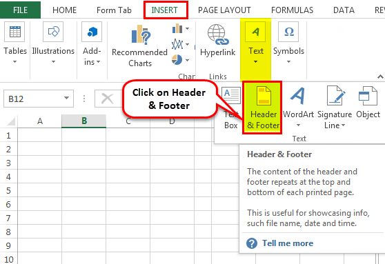
Go to the Insert tab.
Pull-down on Text and select Header & Footer.

Header & Footer Button

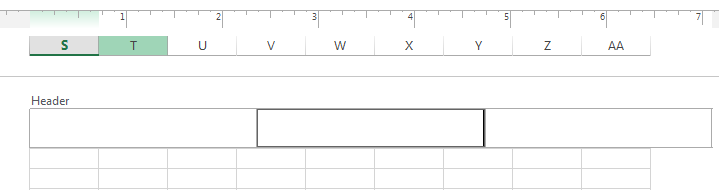
You can find that both headers and footers in your sheet are divided into 3 sections each. This allows you to add up to three header titles or footers to a sheet.

Removing or deleting a header and footer

To remove a header or footer, follow these steps.

Removing Header/Footer from Page Setup Options

Click on the cells in the sheet and not on the header or footer.
Go to the Page Layout tab.
Open the page formatting options by clicking the Page Setup icon at the lower right.
Go to the Header/Footer tab and select (none) for both header and footer.
Click OK.

You can now find that your headers have been removed from all pages in a sheet.

Another way to remove all headers and footers is as follows.

(none) Option in Design Tab

Click on the header or footer.
Go to the Design tab.
Pull-down on Header and press (none) to remove the header.
Pull-down on Footer and press (none) to remove the footer.

1. Adding custom or predetermined texts in header or footer

Let’s see how we can use and modify headers and footers in Excel.

Header Inserted to a Sheet

Let us name this new header and footer with our preferred name
Click the header.
Go to the Design tab.
Under Header & Footer group, pull-down on Header.
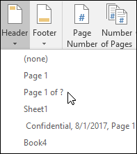
Select a predetermined heading from this list if you cannot decide.

Predetermined Header Texts

To add a custom or predetermined footer text, do as follows next.

Click on the footer.
Type a custom text you want in the footer, or
Go to the Design tab.
Under Header & Footer group, pull-down on Footer.
Select a predetermined text from this list if you cannot decide.

Predetermined Footer Texts

2. Customizing header and footer texts

To customize the header or footer text, follow these steps.

Select the header text.
Go to the Home tab.
Adjust font settings under Fonts group.

Any changes you make to the header get reflected on every single page in Excel. Let’s add some content to all three sections of the header.

Custom Header Text

You can see that we have created and two headings and inserted a page number in the right section.

3. Navigating between headers and footers in Excel

To navigate from the header to the footer or back, do as follows next.

Go to Footer Button

If you’re in the header, then click on the header.
Go to the Design tab.
Under Navigation, select Go to Footer.
If you’re in the footer, then click on the footer.
Go to the Design tab.
Under Navigation, select Go to Header.

This way you can easily navigate from the header to the footer and back.

4. Insert page numbers to header or footer

To add page numbers to headers and footers in Excel, do as follows.

Click on any header or footer section you want to insert page numbers to.
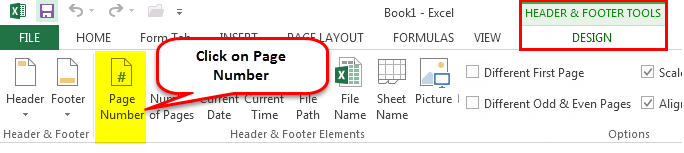
Go to the Design tab, under Header & Footer Elements, select Page Number.

Page Number Button

You can now see that page numbers have been inserted to all pages, and they change as you move to the next page in a sheet and only if there is any content present on the next page.

Page Number Displayed in Header (Right)

5. Inserting number of pages to header or footer

To add a total page count in the header or footer, do as follows.

Number of Pages Button

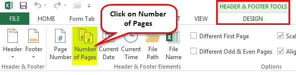
In the Design tab, under the Header & Footer Elements group select Number of Pages.
You can manually type “Pages” after &[Pages] for better understanding.

Header Displaying Number of Pages (Left)

You can see that the header and footer now display the total number of pages.

6. Insert current date to header or footer

To insert the current date in the header or footer, here are the steps.

Current Date Button

In the Design tab, under the Header & Footer Elements group select Current Date.

Footer Displaying Current Date (Left)

You can now see the current date is displayed here in the footer.

7. Insert current time to header or footer

To insert the current time in the header or footer, do as follows.

Current Time Button

In the Design tab, under the Header & Footer Elements group select Current Time.

Current Time Displayed in Footer (Left)

You can now see the current time is displayed in the footer in the image above.

8. Inserting current file path or location to header or footer

To insert the current location of your Excel workbook in the header or footer, do as follows.

File Path Button

In the Design tab, under the Header & Footer Elements group select File Path.

File Path Displayed in Footer (Right)

You can now see the file location or file path is displayed in the footer in the image above.

9. Inserting file name to header or footer

To insert the file name in the header or footer, do as follows.

File Name Button

In the Design tab, under the Header & Footer Elements group select File Name.

Footer Displaying File Name (Right)

You can now see the file name is displayed in the footer.

10. Inserting sheet name to headers and footers in Excel

To insert the current sheet name in the header or footer, do as follows.

Sheet Name Button

In the Design tab, under the Header & Footer Elements group select Sheet Name.

Sheet Name Displayed in Footer (Right)

You can now see the sheet name is displayed in the footer.

How to Add Watermark in an Excel Sheet?

You can easily add a watermark to your Excel worksheet and protect your data from being copied or stolen after getting printed.

You can add an image watermark in Excel to protect your data. Let’s learn it with the help of the steps below.

Header & Footer Button

Open an Excel file.
Go to the Insert tab.
Pull-down on Text and select Header & Footer.
Click on the middle header section if you want to place the watermark in the middle of the sheet.
Now, to add an image watermark, go to the Design tab.
Click on Picture, under the Header & Footer Elements group.
A window named Insert Pictures opens where you can choose to upload an image from your system files, Bing image search, or your personal OneDrive account.

Insert Pictures Window

Once you’ve selected your watermark image, this is what you will see in the header.

Picture Inserted in Header

Do not worry, this is normal. You can adjust the position of your watermark by pressing ENTER before &[Picture] until you reach the desired position, like this.

Adjusting Picture Position

Click outside the white box to view the image.

This is how our image watermark looks like after applying.

Watermark Applied to Sheet

This image looks quite small, here are the steps to increase the size of your watermark in Excel.

Click on the header section with the picture inserted.
Go to the Design tab.
Select Format Picture under Header & Footer Elements.
A window named Format Picture opens where you can adjust the size under the Size tab.
You can even adjust the brightness or transparency of your watermark under the Picture tab.

Adjust Picture Size & Brightness

Hit OK when you’re done.

Resized Watermark

You can now see that the watermark has been resized to a larger size.

Conclusion

This article was all about adding, removing, and modifying headers, footers, and watermarks in Microsoft Excel. If you have any doubts regarding the topics discussed above, feel free to comment below, and we will help you out!

Reference: Microsoft

Источник

Download Article

The definitive guide to adding columns headers to your Excel spreadsheet

Download Article

Keeping the Header Row Visible

Printing a Header Row Across Multiple Pages

Creating a Header in a Table

Add and Rename Headers in Power Query

Tips

This wikiHow will show you how to add a header row in Excel. There are several ways that you can create headers in Excel, and they all serve slightly different purposes. You can freeze a row so that it always appears on the screen, even if the reader scrolls down the page. If you want the same header to appear across multiple pages, you can set specific rows and columns to print on each page. If your data is organized into a table, you can use headers to help filter the data. If you imported a dataset using Power Query, you can change the first row into column headers.

Things You Should Know

Freeze a row by going to View > Freeze Panes.
Print a row across multiple pages using Page Layout > Print Titles.
Create a table with headers with Insert > Table. Select My table has headers.
Add headers to a Power Query table: Query > Edit > Transform > Use First Row as Headers.

1
Select a cell in the row you want to freeze. You can set Excel to freeze your header row so it’s always visible, even as you scroll.
- If your header row is in row 1, you don’t have to click any cells. Just continue to the next step.
- If your header row is down further, such as in row 2 or 3, click a cell below the header row.
  - For example, if the row that contains your column labels is row 5, you will need to click a cell in row 6.
2

Click the View tab. You’ll see it at the top of the window.

Advertisement
3

Click Freeze Panes. This menu is in the toolbar at the top of Excel. A list of freezing options will appear.
4
Select a Freeze Pane option. The option you select on this menu depends on whether your header row is in row 1 or in a different row:
- If your header row is in row 1 (the first row on your sheet), select Freeze Top Row. This ensures that the top row of your sheet remains locked into position, even as you scroll through your data.
- If your header row is in a different row, such as row 3, select Freeze Panes. This freezes the row above the cell you selected in Step 1.
  - For example, if you selected A6 in Step 1, selecting Freeze Panes will freeze row 5, making it your header row. This row will always stay visible as you scroll through your data.
- The Freeze Panes option works as a toggle. That is, if you already have panes frozen, clicking the option again will unfreeze your current setup. Clicking it a second time will refreeze the panes in the new position.
5

Add emphasis to your header row (optional). Create a visual contrast for this row by centering the text in these cells, applying bold text, adding a background color, or drawing a border under the cells. this can help the reader take notice of the header when reading the data on the sheet.

1

Click the Page Layout tab. If you have a large worksheet that spans multiple pages that you need to print, you can set a row or rows to print at the top of every page.
2

Click the Print Titles button. You’ll find this in the Page Setup section.
3

Set your Print Area to the cells containing the data. Click the button next to the Print Area field and then drag the selection over the data you want to print. Don’t include the column headers or row labels in this selection.
4

Click the button next to «Rows to repeat at top.» This will allow you to select the row(s) that you want to treat as the constant header.
5

Select the row(s) that you want to turn into a header. The rows that you select will appear at the top of every printed page. This is great for keeping large spreadsheets readable across multiple pages.
6

Click the button next to «Columns to repeat at left.» This will allow you to select columns that you want to keep constant on each page. These columns will act like the rows you selected in the previous step, and will appear on every printed page.
7
Set a header or footer (optional). You can include the company title or document title at the top, and insert page numbers at the bottom. This will help the reader get the pages organized. To set the header and footer:
- Click the Header/Footer tab
- Click the Header or Footer drop down menus to select a preset header.
- Alternatively, click Custom Header or Custom Footer to create your own.
8
Print your sheet. You can send the spreadsheet to print now, and Excel will print the data that you set with the constant header and columns you chose in the Print Titles window.
- Click Print to start the printing process.
- Check the print preview in the preview section.
- Click Print (the printer icon) to print the spreadsheet.

1
Select the data that you want to turn into a table. When you convert your data to a table, you can use the table to manipulate the data. One of the features of a table is the ability to set headers for the columns. Note that these are not the same as worksheet column headings or printed headers.
- For example, if you’re using Excel to track your bills, you might have headers like Date, Expense Type, and Amount.
2
Click the Insert tab and click Table. Confirm that your selection is correct.
- If you’re looking for Pivot Table information, check out our intro guide here.
3
Check the «My table has headers» box and click OK. This will create a table from the selected data. The first row of your selection will automatically be converted into column headers.
- If you don’t select «My table has headers,» a header row will be created using default names. You can edit these names by selecting the cell.
4
Enable or disable the header. This will show or hide the header. It won’t delete the header information, so you can turn it on and off as needed.^[1]
- Click the Design tab
- Check or uncheck the «Header Row» box to toggle the header row on and off. You can find this option in the Table Style Options section of the Design tab.
- Note that turning the header off will also remove any applied filters from the table.

1
Select a cell in your imported data. This will cause the “Table Design” and “Query” tabs to appear at the top of Excel. This method is used to add row headers to the dataset you imported using Get & Transform (Power Query). You’ll also be able to rename existing headers using this method.^[2]
- Note that this method requires the first row of your dataset to contain column header names.
2

Click Query. This is the rightmost tab at the top of Excel.
3

Click Edit in the Query tab. This is the icon with a spreadsheet and pencil. The Power Query Editor window will open.
4

Click Transform. This is a tab at the top of the Power Query Editor.
5
Make the first row of data the header. To do so:
- Click Use First Row as Headers.
- Select Use First Row as Headers in the drop down menu. This will make row 1 into the headers for the table.
6
Rename the headers. In the Power Query Editor, you can rename the column headers using these steps:
- Double-click the column header name.
- Type in a new name for the header.
- Press ↵ Enter to confirm the name.
7

Click Close & Load in the Home tab of the editor. This will reload the imported table with the changes you made in the editor.

Add New Question

Question

How do I get my headers to change the dates and days automatically?

Use the function @Today. You’ll find it near the top under the choice «Functions».

Ask a Question

200 characters left

Include your email address to get a message when this question is answered.

Submit

Most errors that occur from using the Freeze Panes option are the result of selecting the header row instead of the row just beneath it. If you receive an unintended result, remove the «Freeze Panes» option, select 1 row lower and try again.

Thanks for submitting a tip for review!

About This Article

Article SummaryX

1. Click the View tab.
2. Select the corner cell under the header row.
3. Click Freeze Panes.
4. Apply formatting to the header row.

Did this summary help you?

Thanks to all authors for creating a page that has been read 1,049,311 times.

Is this article up to date?

Источник

The header and footer are the document’s top and bottom portions, respectively. Similarly, Excel also has options for headers and footers. They are available in the “Insert” tab in the “Text” section. Using these features can provide us with two different spaces in the worksheet, one on the top and one on the bottom.

A header in excel: A worksheet section appears at the top of each Excel sheet or document page. It remains constant across all the pages. For example, it can contain page no., date, title, chapter name, etc.

Footer in Excel: A worksheet section appears at the bottom of each page in the Excel sheet or document. It remains constant across all the pages. It can contain page no., date, title, chapter name, etc.

The purpose of Header and Footer in Excel

The purpose is similar to that of hard copy documents or books. The headers and footers in Excel help meet the standard representation format of the documents and/or worksheets. In addition, they add a sense of organization to the soft documents and/or worksheets.

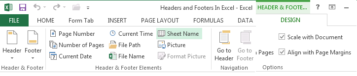
As we can see in the screenshot above, there are four sections under header and footer tools: “Header & Footer,” “Header & Footer Elements,” “Navigation,” and “Options.” This toolbox appears after clicking “Insert”-> “Header & Footer.”

Header & Footer – This shows a list of the quick options as a header or footer.
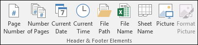
Header & Footer Elements – This has options for the text to be used as a header or footer, such as “Page Number,” “File Name,” “Number of Pages,” etc.
Navigation – It has two options: “Go to Header” and “Go to Footer,” which navigates the cursor to the respective area.
Options – It has two options related to putting up the header and footer conditionally: Different on the first page and Different on Odd & Even page. The other two options are regarding the formatting of the excelFormatting is a useful feature in Excel that allows you to change the appearance of the data in a worksheet. Formatting can be done in a variety of ways. For example, we can use the styles and format tab on the home tab to change the font of a cell or a table.read more page. One is to scale the header/footer with the document. The other is to align the header/footer with page margins.

What are the Header and Footer in Excel?
- Header & Footer Tools in Excel
  - How to Create a Header in Excel?
  - How to Create Footer in Excel?
  - How to Remove Header and Footer in Excel?
  - How to Put Custom Text in Excel Header?
  - How to Assign Page Number in Excel Footer Text?
- Things to Remember
- Recommended Articles

Following are the steps for creating a header in Excel:

First, click the worksheet where we want to add or change the header. Then, go to the “Insert tab” -“Text” group – “Header & Footer.”
Clicking on it would open a new window, as shown below.
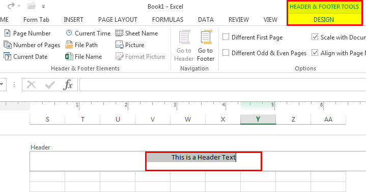
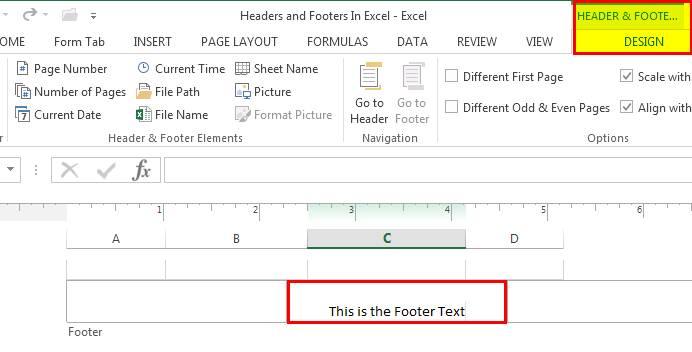
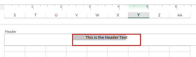
As shown in the screenshot below, “Header & Footer Tools” has a “Design” tab containing various text options to put as the header. The default is an empty text box wherein we can enter a free text, e.g., “This is the header text.” The other options are “Page Number,” “Number of Pages,” “Current Date,” “Current Time,” “File Path,” “File Name,” “Sheet Name,” “Picture,” etc.

We must first click the worksheet where we want to add or change the header. Then, go to the “Insert” tab -> “Text” group -> “Header & Footer.”

Clicking on it would open a new window, as shown. As shown in the screenshot below, “Header & Footer Tools” has a “Design” tab containing various text options to put as the header. The default is an empty text box wherein you can enter a free text, e.g., “This is the Footer text.” The other options are “Page Number,” “Number of Pages,” “Current Date,” “Current Time,” “File Path,” “File Name,” “Sheet Name,” “Picture,” etc.

How to Remove Header and Footer in Excel?

We must first launch the “Page Setup” dialog box from the “Page Setup” box under the “Page Layout” menu.

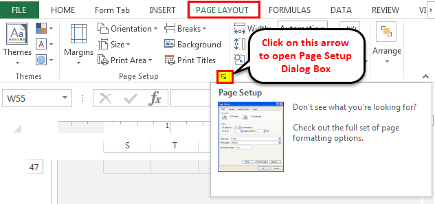
Then, go to the “Header/Footer” section.

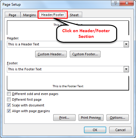
Select ‘none’ for “Header” and/or “Footer” to remove the respective feature.

How to Put Custom Text in Excel Header?

In the following example, “This is the Header Text” is the custom text entered in the “Header” box. The same will reflect on all the pages in the worksheet.

The “Header Text Editor” can be closed by pressing the “Escape” key on the keyboard.

How to Assign Page Number in Excel Footer Text?

The figure shows that a page number can be entered as the footer text. Refer to the screenshot below to understand the same.

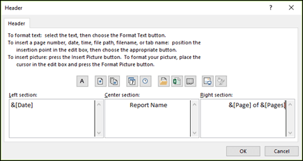
In the following example, “Page [&page] Of [&page]” is the text entered in the “Footer” box. Here, the “&[Page]Of” is a dynamic parameter that evaluates the page number. The first parameter is the current page number, and the second is the total number of pages. The same will reflect on all the pages in the worksheet.

To give page numbers to a sheet, we must click on a sheet, go to “Footer,” click on the “Design” tab under “Header & Footer Tools,” and select “Page Number.”

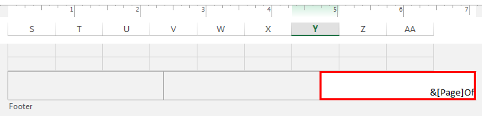
After “Selecting Page Numbers,” it will display as “&[Page]Of,” as shown in the below screenshot.

To show page numbers with total numbers of pages, we must click on the number of pages under the “Design” tab in the “Header & Footer” tool.

After selecting the number of pages, it will add “&[Page] Of &[Pages].

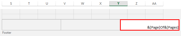
Then it shows the page number with the number of pages.

The “Footer Text Editor” can be closed by pressing the “Escape” key on the keyboard.

Note: In addition to the above-explained examples, the other options for header/footer text made available by MS Excel are “Date,” “Time,” “File Name,” “Sheet Name,” etc.

Things to Remember

The headers and footers in Excel help meet the standard representation format of the documents or worksheets.
They add a sense of organization to the soft documents.
Excel offers various options to be put up as header/footer text, such as “Date,” “Time,” “Sheet Name,” “File Name,” “Page Number,” “Custom Text,” etc.

Add or change headers or footers in Page Layout view

Need more help?

See Also

Need more help?

How do I make the first row in Excel a column header?

How do I create a column header row in Excel?

How do you make a title for a sheet?

How do I freeze a row in Excel?

What are column headers?

What is footer and header?

How do you name a spreadsheet in Google Sheets?

How do I change the title of a Google sheet?

Can you freeze a row and a column in Excel?

How do you freeze 3 rows in Excel?

How do I run goal seek in Excel?

How do I make column headers in Google Sheets?

How do I make the top row of Google Sheets always visible?

How to Add or Remove Headers and Footers in Excel?

Adding a header and footer

Removing or deleting a header and footer

1. Adding custom or predetermined texts in header or footer

2. Customizing header and footer texts

3. Navigating between headers and footers in Excel

4. Insert page numbers to header or footer

5. Inserting number of pages to header or footer

6. Insert current date to header or footer

7. Insert current time to header or footer

8. Inserting current file path or location to header or footer

9. Inserting file name to header or footer

10. Inserting sheet name to headers and footers in Excel

How to Add Watermark in an Excel Sheet?

Conclusion

Things You Should Know

About This Article

Is this article up to date?

Table of contents

How to Remove Header and Footer in Excel?

How to Put Custom Text in Excel Header?

How to Assign Page Number in Excel Footer Text?

Things to Remember

Recommended Articles