
Group or ungroup data in a PivotTable
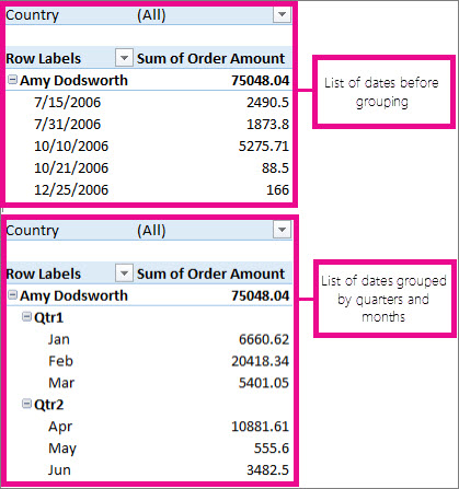
Grouping data in a PivotTable can help you show a subset of data to analyze. For example, you may want to group an unwieldy list date and time fields in the PivotTable into quarters and months

-
In the PivotTable, right-click a value and select Group.
-
In the Grouping box, select Starting at and Ending at checkboxes, and edit the values if needed.
-
Under By, select a time period. For numerical fields, enter a number that specifies the interval for each group.
-
Select OK.
-
Hold Ctrl and select two or more values.
-
Right-click and select Group.
With time grouping, relationships across time-related fields are automatically detected and grouped together when you add rows of time fields to your PivotTables. Once grouped together, you can drag the group to your Pivot Table and start your analysis.
-
Select the group.
-
Select Analyze > Field Settings. In the PivotTable Analyze tab under Active Field click Field Settings.
-
Change the Custom Name to something you want and then select OK.
-
Right-click any item that is in the group.
-
Select Ungroup.
-
In the PivotTable, right-click a value and select Group.
-
In the Grouping box, select Starting at and Ending at checkboxes, and edit the values if needed.
-
Under By, select a time period. For numerical fields, enter a number that specifies the interval for each group.
-
Select OK.
-
Hold Ctrl and select two or more values.
-
Right-click and select Group.
With time grouping, relationships across time-related fields are automatically detected and grouped together when you add rows of time fields to your PivotTables. Once grouped together, you can drag the group to your Pivot Table and start your analysis.
-
Select the group.
-
Select Analyze > Field Settings. In the PivotTable Analyze tab under Active Field click Field Settings.
-
Change the Custom Name to something you want and then select OK.
-
Right-click any item that is in the group.
-
Select Ungroup.
Need more help?
You can always ask an expert in the Excel Tech Community or get support in the Answers community.
See Also
Create a PivotTable to analyze worksheet data
Need more help?
The ability to quickly group dates in Pivot Tables in Excel can be quite useful.
It helps you analyze data by getting different views by dates, weeks, months, quarters, and years.
For example, if you have credit card data, you may want to group it in different ways (such as grouping by months or quarters or years).
Similarly, if you have a call center data, then you may want to group it by minutes or hours.
Watch Video – Grouping Dates in Pivot Tables (Grouping by Months/Years)
How to Group Dates in Pivot Tables in Excel
Suppose you have a dataset as shown below:
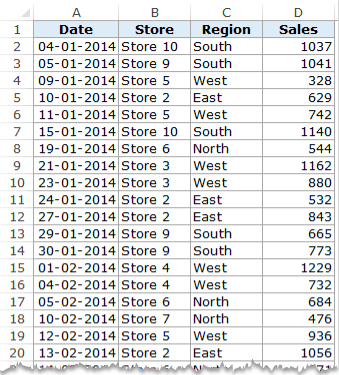
It has sales data by Date, Stores, and Regions (East, West, North, and South). The data spans across 300+ rows and 4 columns.
Here is a simple pivot table summary created using this data:
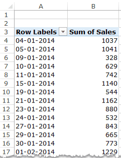
This pivot table summarizes sales data by date, but it isn’t quite helpful as it shows all the 300+ dates. In such as case, it would be better to have the dates grouped by years, quarters, and/or months
Download Data and follow along.
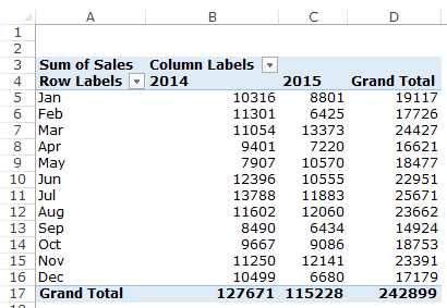
Grouping by Years in a Pivot Table
The dataset shown above have dates for two years (2014 and 2015).
Here are the steps to group these dates by years:
This would summarize the pivot table by years.

This summarization by years may be useful when you have more number of years. In this case, it would be better to have the quarterly or monthly data.
Grouping by Quarters in a Pivot Table
In the above dataset, it makes more sense to drill down to quarters or months to have a better understanding of the sales.
Here is how you can group these by quarters:
This would summarize the pivot table by quarters.

The issue with this pivot table is that it combines the Quarterly sales value for 2014 as well as 2015. Hence, for each quarter, the sales value is the sum of sales values in Quarter 1 in 2014 and 2015.
In a real life scenario, you are most likely to analyze these quarters for each year separately. To do this:
This would summarize the data by Years and then within years by Quarters. Something as shown below:
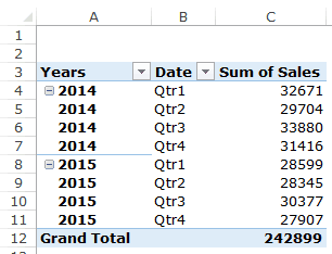
Note: I am using the tabular form layout in the above snapshot.
When you group dates by more than one time-frame group, something interesting happens. If you look at the field list, you will notice a new field has automatically been added. In this case, it is Years.
Note that this new field that has appeared is not a part of the data source. This field has been created in the Pivot Cache to quickly group and summarizes data. When you ungroup the data, this field will vanish.
The benefit of having this new field is that now you can analyze the data with quarters in rows and years in columns, as shown below:

All you need to do is drop the Year field from Row area to Columns area.

Grouping by Months in a Pivot Table
Similar to the way we grouped the data by quarters, we can also do this by months.
Again, it is advisable to use both Year and Month to group the data instead of only using months (unless you only have data for one or less than a year).
Here are the steps to do this:
- Select any cell in the Date column in the Pivot Table.
- Go to Pivot Table Tools –> Analyze –> Group –> Group Selection.
- In the Grouping dialogue box, select Months as well as Years. You can select more than one option by simply clicking on it.

- Click OK.

This would group the date field and summarize the data as shown below:

Again, this would lead to a new field of Years getting added to the PivotTable fields. You can simply drag the years’ field to the columns area to get the years in columns and months is rows. You will get something as shown below:
Grouping by Weeks in a Pivot Table
While analyzing data such as store sales or website traffic, it makes sense to analyze it on a weekly basis.
When working with dates in Pivot Tables, grouping dates by week is a bit different than grouping by months, quarters, or years.
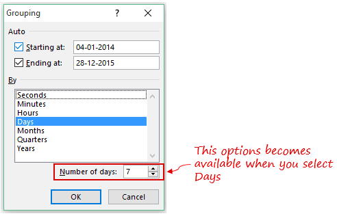
Here is how you can group dates by weeks:
- Select any cell in the Date column in the Pivot Table.
- Go to Pivot Table Tools –> Analyze –> Group –> Group Selection.

- In the Grouping dialogue box, select Days and deselect any other selected option(s). As soon as you do this, you would notice that the Number of Days option (at the bottom right) becomes available.
- There is no inbuilt option to group by weeks. You need to group by days and specify the number of days to be used while grouping.
- Note that for this to work, you need to select Days option only.
- In Number of days, enter 7 (or use the spin button to make the change).

- If you click OK at this point, your data would be grouped by weeks starting with January 4, 2014 – which is a Saturday. So the grouping would be from Saturday to Friday every week. To change this grouping and to begin the week from Monday, you need to change the start date (by default it picks the start date from the source data).
- In such a case, you can either start the date on December 30, 2013, or January 6, 2014 (both Mondays).
- Click OK.

This will group the dates by weeks as shown below:

Similarly, you can group dates by specifying any other number of days. For example, instead of weekly, you can group dates in a biweekly interval.
Note:
- When you group dates by using this method, you can not group it using any other option (such as months, quarters or years).
- Calculated field/item would not work when you group using Days.
Grouping by Seconds/Hours/Minutes in a Pivot Table
If you working with high volumes of data (such as call center data), you may want to group it by seconds or minutes or hours.
You can use the same process to group the data by seconds, minutes, or hours.
Suppose you have the call center data as shown below:

In the above data, the date is recorded along with the time. In this case, it may make sense for the call center manager to analyze how the call resolve numbers are changing per hour.
Here is how to group the days by Hours:
This will group the data by hours and you will get something as shown below:

You can see that the Row Labels here are 09, 10, and so on.. which are the hours in a day. 09 would mean 9 AM and 18 would be 6 PM. Using this pivot table, you can easily identify that most calls are resolved during 1-2 PM.
Similarly, you can also group the dates on seconds and minutes.
How to Ungroup Dates in a Pivot Table in Excel
To ungroup dates in pivot tables:
- Select any cell in the date cells in the pivot table.
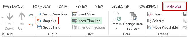
- Go to PivotTable Tools –> Analyze –> Group –> Ungroup.

This would instantly ungroup any grouping that you have done.
Download the Example File.
Other Pivot Table Tutorials You May Like:
- Creating a Pivot Table in Excel – A Step by Step Tutorial.
- Preparing Source Data For Pivot Table.
- How to Group Numbers in Pivot Table in Excel.
- How to Filter Data in a Pivot Table in Excel.
- How to Apply Conditional Formatting in a Pivot Table in Excel.
- How to Refresh Pivot Table in Excel.
- How to Add and Use an Excel Pivot Table Calculated Field.
- Using Slicers in Excel Pivot Table.
- How to Replace Blank Cells with Zeros in Excel Pivot Tables.
- Count Distinct Values in Pivot Table
Before I was a Pivot Table guru, I had to get individual rows of daily sales and group them into a report showing the monthly sales during the year.
Group Dates in Pivot Table would take a ton of effort using Formulas:
- Extracting the month and year from each transactional date;
- Then manually grouping them together to get the total sales numbers for each month. PAINFUL & SLOW!
Thankfully there is the Pivot Table way (I wish I had known this back then), which is quick and reduces the risks of making any errors….ah yeah & I almost forgot, it is also easy to add new data to your sales report with a simple Refresh!
In this article, we will be covering the following topics in detail:
- Group Dates in Pivot Table by Month & Year
- Group Dates in Pivot Table by Week
- Summarize Value by
- Change Formatting
- Control Automatic Grouping
Let’s look at each one of these!
Group Dates in Pivot Table by Month & Year
In the data below, you can see that there are two columns: one that contains the transaction date of the sale, and the second column contains the total sales amount for a particular date.

Want to know How To Group Dates in Pivot Table by Month?
In the example below, I show you how to Pivot Table Group by Month:
STEP 1: Insert a new Pivot table by clicking on your data and going to Insert > Pivot Table > New Worksheet or Existing Worksheet

STEP 2: In the ROWS section put in the Order Date field.
Notice that in Excel 2016 (the version that I am using) it will automatically Group the Order Date into Years & Quarters:

STEP 3: Right-click on any row in your Pivot Table and select Group so we can select our Group order that we want:

STEP 4: We need to deselect Quarters and make sure only Months and Years are selected (which will be highlighted in blue).
This will group our dates by the Months and Years. Click OK.

STEP 5: In the VALUES area put in the Sales field. This will get the total of the Sales for each Month & Year:

This is how you can easily create Pivot Table Group Dates by Month!

Group Dates in Pivot Table by Week
To group the dates by week, follow the steps below:
STEP 1: Right-click on one of the dates and select Group.

STEP 2: Select the day option from the list and deselect other options.

STEP 3: In the Number of days section, type 7.

This is how the group dates in Pivot Table by week will be displayed.

STEP 4: You can even change the starting date to 01-01-2012 in the section below.

Your final grouped data is ready!

Change Formatting
Now we have our sales numbers grouped by Month & Years, notice that we can improve the formatting by following the steps below:
STEP 1:Click the Sum of SALES and select Value Field Settings

STEP 2: Select Number Format

STEP 3: Select Currency. Click OK.

You now have your total sales for each monthly period! Quick & Easy!

Summarize Value by
In the previous examples, you saw how to get total sales by month, year, or week. You can even calculate the total number of sales that occurred in a particular month, year, or week.
Let’s look at an example to know how:
STEP 1: Right-click anywhere on the Pivot Table.

STEP 2: Select Value Field Settings from the list.

STEP 3: In the Value Field Setting dialog box, select Count.

STEP 4: Click OK.

This will summarize the values as a count of sales instead of the sum of sales (like before).

Ungroup Dates
To ungroup dates in a Pivot Table, simply right-click on the dates column and select ungroup.

Or, you can go to the PivotTable Analyze tab and select Ungroup.

Once this is done, the data will be ungrouped again.
Control Automatic Grouping
If you wish to, you can easily turn off this automatic date grouping feature in Excel 2016. To do that, follow the steps below:
STEP 1: Go to File Tab > Options

STEP 2: In the Excel Options dialog box, click Data in the categories on the left.

STEP 3: Check Disable automatic grouping of Date/Time columns in PivotTables checkbox.

STEP 4: Click OK.

This will easily turn off the automatic grouping feature in the Pivot Table! So, the date will be not be grouped automatically now when you drag the date field to an area in the pivot table.
Conclusion
You can easily analyze data by week, month, year, days, hour, etc., and find trends using this grouping dates feature in Pivot Table. It is a fairly simple and super quick method to group dates.
Did you know there are many creative ways of doing grouping in Excel Pivot Tables?
Learn all about it here!
About The Author
Bryan
Bryan is a best-selling book author of the 101 Excel Series paperback books.
Group Dates in an Excel Pivot Table by Month and Year
by Avantix Learning Team | Updated March 7, 2021
Applies to: Microsoft® Excel® 2013, 2016, 2019 and 365 (Windows)
If you have valid dates entered in your source data, you can group by month, year or other date period in a pivot table in Excel. There are two common approaches to grouping by date. You can group by date periods in a pivot table using the Grouping feature (this may occur automatically depending on your version of Excel). Alternatively, you can also create calculations in source data to extract the month name and the year from a date field and use the fields in your pivot table.
Recommended article: How to Delete Blank Rows in Excel Worksheets (Great Strategies, Tricks and Shortcuts)
Do you want to learn more about Excel? Check out our virtual classroom or live classroom Excel courses >
Source data is typically entered vertically with data in columns and field names at the top of each column of data.
Grouping by month and year in a pivot table
The key to grouping by month and/or year in a pivot table is a source field with valid dates (such as OrderDate). Depending on your Control Panel settings on your device, valid dates may be entered as month/day/year, day/month/year or year/month/day (although they can be formatted to appear in other ways).
In Excel 2016 and later versions, if you drag a date field into the Rows or Columns area of a pivot table, Excel will group by date increments by default.
The easiest way to group by a date period is to right-click in a cell in a date field in a pivot table and select the desired grouping increments. You can group dates by quarters, years, months and days. The source data does not need to contain a year, quarter or month name column.
To group by month and/or year in a pivot table:
- Click in a pivot table.
- Drag a date field into the Row or Columns area in the PivotTable Fields task pane.
- Select a date field cell in the pivot table that you want to group. Excel may have created a Year and/or Month field automatically.
- Right-click the cell and select Group from the drop-down menu. You can also right-click a date field in the Rows or Columns area in the PivotTable Fields task pane. A dialog box appears.
- Click the date periods that you want to group by. Select Quarters, Years, Months or Days. You can click on more than one such as Years and Months.
- Click OK.
The Grouping dialog box offers multiple options for grouping by date:

The date field will be grouped and new fields will be added to the field list for the groups (if they didn’t exist beforehand).
In the following example, Excel grouped automatically by date periods in the PivotTable Fields task pane. This occurs in 2016 or later versions:

To remove a grouping period for a date field:
- Select a date field cell in the pivot table that has been grouped.
- Right-click the cell and select Group. You can also right-click a date field in the Rows or Columns area in the PivotTable Fields task pane. A dialog box appears.
- Deselect or click the groups you wish to remove.
- Click OK.
To remove all grouping:
- Select a date field cell in the pivot table that has been grouped.
- Right-click the cell and select Ungroup.
Controlling automatic grouping
In Excel 2016 and later versions, dates are grouped automatically if they are placed in the Rows or Columns area of the pivot table. You can turn this setting off or on.
To disable automatic grouping for pivot tables:
- Click the File tab in the Ribbon.
- Click Options. A dialog box appears.
- Click Data in the categories on the left. If you are using an older version of Excel, click Advanced in the categories on the left.
- Select or check Disable automatic grouping of Date/Time columns in PivotTables checkbox.
- Click OK.
Below is the Excel Options dialog box in 365:

If you disable automatic grouping, you can still right-click and group in pivot tables but the groups will not be created automatically when you drag a date field to an area in the pivot table.
Issues with pivot table cache
When you create a pivot table and group using the Group feature, the fields and the groupings are stored in a pivot cache, not in the source data. This can be problematic if you create more pivot tables based on the same pivot cache. This means that all pivot tables that share the same cache, will also share the date groupings.
There is no easy way to see which pivot tables share the same cache in the Excel. You would need to use VBA (Visual Basic for Applications) to find this information.
You can unshare the cache by changing the source data range, but this can be tricky if you have a lot of pivot tables.
Creating date period fields in the source data
Another option is to create fields in the source data that calculate date periods (such as Year and Month). You can use the YEAR and TEXT functions to extract Year and Month from a valid date field.
For example, if you have a date in column A, you could create a calculation to extract the Year in column B and the Month in column C.
To calculate the year in B2 (assuming there is a valid date in A2), enter the following formula and then copy the formula down:
=YEAR(A2)
To calculate the month name in C2 (assuming there is a valid date in A2), enter the following formula and then copy the formula down:
=TEXT(A2,»mmmm»)
If the source data is in an Excel table, it’s best to use structured referencing formulas in each row such as =YEAR([@OrderDate]) or =TEXT([@OrderDate],»mmmm») where OrderDate is the name of the field and @ is a specifier to refer to the current row or record.
The benefit of creating the fields in the source data is that you can create a pivot table and then group by these fields in the pivot table simply by dragging them into the Rows or Columns area. You will be able to create other pivot tables that do not include the date grouping.
Another advantage of creating fields in the source data is that you can reuse the date period fields in other reports, formulas or slicers.
Summary
The method you choose depends on your needs. We have not used the Power Pivot data model here (which provides another method of grouping by date) but is available only in certain versions of Excel. Also, these methods assume a fiscal year of January to December. You’d need to create other calculations in the source data if you want to sort months by a fiscal year that starts and ends in other months (such as April to March).
Subscribe to get more articles like this one
Did you find this article helpful? If you would like to receive new articles, join our email list.
More resources
10 Great Excel Pivot Table Shortcuts
Excel Flash Fill Tricks to Clean and Extract Data (10 Examples)
How to Change Commas to Decimal Points in Excel and Vice Versa (5 Ways)
3 Excel Strikethrough Shortcuts to Cross Out Text or Values in Cells
Related courses
Microsoft Excel: Intermediate / Advanced
Microsoft Excel: Data Analysis with Functions, Dashboards and What-If Analysis Tools
Microsoft Excel: Introduction to Power Query to Get and Transform Data
Microsoft Excel: New and Essential Features and Functions in Excel 365
Microsoft Excel: Introduction to Visual Basic for Applications (VBA)
VIEW MORE COURSES >
Our instructor-led courses are delivered in virtual classroom format or at our downtown Toronto location at 18 King Street East, Suite 1400, Toronto, Ontario, Canada (some in-person classroom courses may also be delivered at an alternate downtown Toronto location). Contact us at info@avantixlearning.ca if you’d like to arrange custom instructor-led virtual classroom or onsite training on a date that’s convenient for you.
Copyright 2023 Avantix® Learning
Microsoft, the Microsoft logo, Microsoft Office and related Microsoft applications and logos are registered trademarks of Microsoft Corporation in Canada, US and other countries. All other trademarks are the property of the registered owners.
Avantix Learning |18 King Street East, Suite 1400, Toronto, Ontario, Canada M5C 1C4 | Contact us at info@avantixlearning.ca
 Pivot Tables allow you to easily summarize, analyze and present large amounts of data.
However, to appropriately do this, you must be able to organize the data into adequately-sized and organized subsets. The grouping and ungrouping features of Pivot Tables allow you to easily do this.
You see…
Knowing how to quickly group data within a PivotTable report can help you immensely. This is because it allows you easily group a huge amount of disparate data into a few groups or subsets. Fewer groups allow you to simplify your analysis and focus on the (grouped) Items that matter the most.
As explained by Excel guru John Walkenbach in the Excel 2016 Bible:
One of the most useful features of a pivot table is the ability to combine items into groups.
This Pivot Table Tutorial explains all the details you need to know to group and ungroup data in a Pivot Table. I focus on showing how you can easily group different types of Fields in different circumstances. You can also find a thorough explanation of how to ungroup data. Finally, I explain how to solve some of the most common problems and challenges you may encounter when trying to group Pivot Table data.
The following table of contents lists the main contents I cover in the blog post below.
Let’s start by looking at the…
Example Pivot Table And Source Data
This Pivot Tutorial is accompanied by an Excel workbook example. If you want to follow each step of the way and see the results of the processes I explain below, you can get immediate free access to this workbook by subscribing to the Power Spreadsheets Newsletter.
I use the following source data for all the examples within this Pivot Table Tutorial. This is similar to the data in other Pivot Table Tutorials, such as this one.

The table contains 20,000 rows. It lists the following sales data:
- Date: Between January 1 of 2017 and December 31 of 2019.
- Item: Any of the following Microsoft products:
- Surface Studio.
- Surface Book.
- Surface Pro 4.
- Xbox One S.
- Xbox One.
- Store: I assume there’s only 1 store per city. The city can be any of the following:
- Atlanta.
- Boston.
- Chicago.
- Dallas.
- Detroit.
- Houston.
- Los Angeles.
- Miami.
- Minneapolis.
- New York.
- Philadelphia.
- Phoenix.
- San Diego.
- San Francisco.
- Seattle.
- Tampa.
- Washington D.C.
- Units Sold: Between 1 and 5 per entry.
- Unit Price: I assume the following unit prices per item:
- Surface Studio: $2,999.00.
- Surface Book: $1,499.
- Surface Pro 4: $899.
- Xbox One S: $299.
- Xbox One: 249.
- Sales Amount: I calculate this as the product of (i) Units Sold, times (ii) Unit Price:
Units Sold x Unit Price
How To Group Items In A Pivot Table
You can generally group Items in a Pivot Table in 2 different ways:
- Automatically.
- Manually.
The grouping option that’s more suitable for a situation depends on the type of data you’re working with. Consider the following:
- Not all Fields are suitable for automatic grouping.
- The types of Fields that you can usually group automatically are those that hold the following data:
- Numeric.
- Date and/or time.
If you’re working with Excel 2016, there’s an additional grouping feature you can use: automatic date and time column grouping.
Pivot Table grouping is quite flexible. It allows you to group several different types of Fields. You can create many groups and you can group previously existing groups (create groups of groups).
Despite its flexibility, Pivot Table grouping has some restrictions. Note the following 2 limitations:
- You can’t add Calculated Items to grouped Fields. If you want to add a Calculated Item, proceed in the following 3 steps:
- Ungroup the Field.
- Add the Calculated Item(s).
- Regroup the Field.
- Even though this Pivot Table Tutorial doesn’t focus on Online Analytical Processing (OLAP) sources, there are certain important restrictions/issues to consider. I provide some more comments about these in an individual section below.
In the following sections, I provide a detailed explanation of each of the different ways of grouping data in a Pivot Table.
How To Automatically Group Date Or Time Fields In An Excel 2016 Pivot Table
In Excel 2016, Microsoft introduced the time grouping feature.
Time grouping is generally triggered when you add a date or time Field to either the Rows or Columns Areas of a Pivot Table report.

Once this happens, time grouping proceeds as follows:
- Excel automatically detects relationships across the Field.
For example, as explained by Excel MVP Bill Jelen (Mr. Excel) in Excel 2016 in Depth:
If your data spans a short period within one month, AutoGroup does not take any action. If your data spans several months but does not fall outside of one year, AutoGroup groups to months.
- The Fields are grouped based on the relationships identified in step #1 above. This in turn, results in the following:
- Excel adds calculated columns or rows to group the Field data.
- The data is automatically arranged so that the highest-level date or time period is displayed first.
- The data is generally collapsed.
The above may sound difficult. Don’t worry. The example below shows how this looks in practice.
The main point I’m trying to make is this:
You can automatically group date or time Fields in an Excel 2016 Pivot Table in 1 single easy step:
- Add a date or time Field to the Rows or Columns Areas of the Pivot Table.
Let’s see how this looks in practice:
Assume you have the following PivotTable report based on the example source data I explain above. It displays the Sum of Units Sold and Sum of Sales Amount for each item.

No information from the Date Field is displayed because the Field isn’t yet in any Area.

You can both (i) add the Date Field to the Rows or Columns Area, and (ii) automatically group the Date Field in a single step. In this case, I add the Date Field to the Columns Area.

The resulting Pivot Table report looks as follows. Notice that, in this case, Excel displays the data at the higher-level date. In this case, that’s years.

Once I expand the groups, the Pivot Table looks as in the screenshot below. Notice that Excel automatically does the following:
- Adds the following 3 columns to the Rows Area: Years, Quarters and Date.
- Organizes the added columns in such a way that the highest-level date period is displayed first. Years appears before Quarters. Quarters is before Date.
- Instead of displaying individual days, Excel displays the data at the month level.

If you’re working with data model Pivot Tables, consider the following restriction: If you drag a date Field that has more than 1,000 rows of data from the Field List to a Pivot Table Area, the Field is removed from the Field List. This allows Excel to display a Pivot Table overriding the 1 million records limitation.
If you automatically group Fields with time grouping, Excel assigns default names and labels to the newly created Fields and groups. I explain how you can modify either of these in a separate section below.
Automatically Group Date Or Time Fields With Time Grouping When Field Already Appears In Pivot Table
You can take advantage of the time grouping feature even if you’ve already added date or time Fields to the same Area.
To understand the situation, consider the following Pivot Table. This is the Pivot Table that appears above after I ungroup the Date Field. Notice that the Date Field:
- Is already included in the Rows Area.
- Displays individual days (isn’t grouped).

In such situations, you can anyway use time grouping. Therefore, you can automatically group date or time Fields in 1 single step:
- Add the date or time Field to the relevant Area of the Pivot Table.
As an example, I add the Date Field to the Rows Area of the Pivot Table report above.

The resulting Pivot Table report (below) is the same as that which I show above. In other words, Excel automatically:
- Adds new columns to the Pivot Table.
- Organizes the columns so that the highest-level period is displayed first.
- Collapses the data in the Date Field. The Date Field shows months instead of individual days.

How To Automatically Group Items In A Pivot Table
If you’re working with version of Excel prior to 2016, you won’t have access to the time grouping feature I explain in the previous section. Even if you can use time grouping, there are cases where this feature won’t be the right tool your job.
Therefore, in this section, I explain the general process for automatic Field grouping.
Generally, you can automatically group Items in a Pivot Table in the following 6 easy steps:
- Right-click on a Field that is suitable for automatic grouping.
- Excel displays a contextual menu.
- Select Group.
- Excel displays the Grouping dialog box.
- Specify the grouping conditions in the Grouping dialog box.
- Click on the OK button.
The process above works through a contextual menu. You can also automatically group Items by using commands in the Ribbon or keyboard shortcuts. In this case, you group the Items in 5 simple steps, as follows:
- Select the Field you want to group automatically.
- Go to Ribbon > Analyze > Group Selection, Ribbon > Analyze > Group Field, or use keyboard shortcuts (“Shift + Alt + Right Arrow”, “Alt, JT, K”, “Alt, JT, R” or “(Shift + F10), G”).
- Excel displays the Grouping dialog box.
- Use the Grouping dialog to specify grouping conditions.
- Click the OK button.
Let’s look at each of the steps and processes above in practice, and some details you can consider when grouping Fields automatically. But first, I introduce the Pivot Table reports that I use for the examples/illustrations within this section:
Automatic Grouping Of Pivot Table Field Examples
For the step-by-step explanation of how to automatically group Fields in a Pivot Table, I use the following 2 report examples. Both reports are based on the example source data that I introduce above:
- Report #1: Displays the following data for each day and item:
- Sum of Units Sold.
- Average of Unit Price.
- Sum of Sales Amount.

- Report #2: Displays the following data for each month and unit price:
- Sum of Units Sold.
- Sum of Sales Amount.


To a certain extent, the PivotTable reports above are already summarizing the 20,000 rows of raw data we’re working with. However, you may want to group your data further. In the following sections I automatically group the following Fields:
- Report #1: Group the Date Field by months, quarters and years.
- Report #2: Group the Unit Price Field in $1,000 intervals.
How To Automatically Group Pivot Table Items Through Contextual Menu
As I explain above, you can automatically group Pivot Table items in different ways. In the following sections, I look at the process of automatically grouping Pivot Table Items by using a contextual menu.
Step #1: Right-Click On A Field That Is Suitable For Automatic Grouping
As I explain above, you can’t automatically group absolutely all Fields. Automatic grouping works well with the following:
- Numeric Fields.
- Date and/or time Fields.
In the examples we’re working with, I right-click on the following:
- The Date Field in Report #1:

- The Unit Price Field in Report #2.


Step #2: Excel Displays A Contextual Menu
After your right-click on a Pivot Table Field suitable for automatic grouping, Excel displays a contextual menu.

Step #3: Select Group
In the contextual menu that Excel displays, select Group.

Step #4: Excel Displays The Grouping Dialog Box
After you select Group, Excel displays the Grouping dialog box. The Grouping dialog box differs slightly depending on whether you’re working with a numeric or a date/time Field, as follows:
- Date/time Field, as in Report #1:

- Numeric Field, as in Report #2:


Step #5: Specify The Grouping Conditions In The Grouping Dialog Box
Within the Grouping dialog box, you can specify the 4 following grouping settings (3 when working with numeric Fields):
- Starting at: Smallest number (for numeric Fields) or first date/time (for date/time Fields) to group by.
- Ending at: Largest number (for numeric Fields) or last date/time (for date/time Fields) to group by.
The value you enter in the Starting at input field (#1 above) must be smaller (for numeric Fields) or earlier (for date/time Fields) than the value you choose for Ending at.
- By: Your entry in the By input field depends on the type of data you’re working with, as follows:
- Numeric Fields: Number that represents the group’s interval size. This type of grouping is commonly used for frequency distributions.
- Date or Time Fields: Select 1 or more of the time periods listed by Excel. You can usually select more than 1 time period for grouping.
- Number of days: This field is active if you work with date/time Fields and choose to group by days in the By field (#3 above). This allows you to group date Fields by a certain number of days.
If you group dates by a certain number days and use the Number of days field (#4 above), you can’t group by other time periods (months, quarters, years) at the same time. I explain how to get around this restriction in a separate section below. You can use the process I explain there to, for example, group by (i) weeks and (ii) months, quarters or years.
In our examples, I choose the following grouping settings:
- Report #1: I group all the available data in quarters and years, by specifying the following conditions:
- Starting at: January 1, 2017 (1/1/2017).
- Ending at: January 1, 2020 (1/1/2020).
- By: Quarters and Years.

- Report #2: I group the Unit Price in $1,000 intervals, as follows:
- Starting at: 0.
- Ending at: 3,000 (enter without the comma: 3000).
- By: 1,000 (enter without the comma: 1000.


Step #6: Click On The OK Button
To confirm your grouping settings, click on the OK button in the lower section of the Grouping dialog box or press the Enter key. Excel groups the Fields accordingly (I show this below).

How To Automatically Group Pivot Table Items Through The Ribbon Or With A Keyboard Shortcut
In this section, I look at a second way to automatically group Pivot Table Items. In this case, you work with the Ribbon.
Step #1: Select The Field You Want To Group Automatically
This step is substantially the same as step #1 I describe above for automatically grouping Pivot Table Items through a contextual menu. The difference is that, instead of right-clicking on the Field, you select it.
The Field must generally be a date/time or numeric Field.
It the example we work with, I select the following Fields:
- Report #1: Date.

- Report #2: Unit Price.


Step #2: Go To Ribbon > Analyze > Group Selection, Ribbon > Analyze > Group Field, Or Use A Keyboard Shortcut
You can launch the Grouping dialog box through the Ribbon through either of the following routes:
- Ribbon > Analyze > Group Selection.

- Ribbon > Analyze > Group Field.


If you don’t want to use the Ribbon, simply use any of the following keyboard shortcuts:
- Shift + Alt + Right Arrow.
- Alt, JT, K.
- Alt, JT, R.
- (Shift + F10), G.
Step #3: Excel Displays The Grouping Dialog Box
The look of the Grouping dialog box differs slightly depending on the type of Field you work with. You generally encounter 1 of the following versions, depending on the Field:
- If you’re working with a date or time Field, such as in Report #1:

- If you work with a numeric Field, as in Report #2:


Step #4: Use The Grouping Dialog To Specify Grouping Conditions
This is the same as step #5 of the process to automatically group Pivot Table Items through a contextual menu (above).
In the Grouping dialog box, you get to specify the following conditions:
- Starting at.
- Ending at.
- By.
- Number of days (if grouping by days).
Elements #1 (Starting at) and #2 (Ending at) determine the following:
- If you work with a date or time Field, the first and last date/time to group by.
- If you work with a numeric Field, the smallest and largest numbers to group by.
Element #3 above (By) also differs slightly depending on whether you work with a date/time or numeric Field, as follows:
- Date/Time Field: By is a list box that allows you to select 1 or more of the time periods that Excel lists.
- Numeric Field: By is an input field where you can specify a number representing the grouping intervals.
Element #4 (Number of days) applies when you group by days. You use it to specify the number of days used to group the data into.
In the example we look at, I enter the following inputs:
- Report #1: My purposes is to group data in quarters and years.
- Starting at: 1/1/2017.
- Ending at: 1/1/2020.
- By: Quarters and Years.

- Report #2: My goal is to group the Unit Price Field in $1,000 intervals.
- Starting at: 0.
- Ending at: 3000.
- By: 1000.


Step #5: Click The OK Button
After you enter the grouping conditions in the Grouping dialog, confirm your input by clicking on the OK button in the lower right corner of the dialog box.

Results Of Automatically Grouping Items In A Pivot Table
The results I obtain in the examples we’re working with are the same regardless of which process of automatic grouping (through a contextual menu vs. the Ribbon) I use. These results look as follows:
- Report #1: Data is grouped in quarters and years:

- Report #2: Data is grouped in $1,000-per-unit price intervals.


Excel assigns default names and labels to any newly created Fields or groups. You can easily modify either of these by following the processes that I explain further below.
How To Group By Weeks (Or Other Number Of Days) And Months, Quarters And/Or Years
The process to automatically group by dates that I explain in the previous section covers most situations.
However, as I explain above, you can’t group by (i) a certain number of days, and (ii) the other grouping periods (months, quarters or years). A common situation where this restriction can be annoying is if you want to group by weeks (7 days) and months, quarters or years.
The most common solution to this problem is to add a helper column to the source data. In other words, you can group by weeks (or other number of days) and months, quarters and/or years in the following 6 easy steps:
- Group the date Field, to the extent possible, using the automatic grouping process I describe above.
- Add helper column(s) to the source data.
- In each helper column, add a formula to calculate grouping levels/intervals.
- Expand the data source of your Pivot Table to include the helper column(s).
- The Pivot Table Field List displays the new Field(s) that correspond to the helper column(s) you added.
- Add the newly-added Field(s) to the Rows or Columns Areas.
In the following sections, I show you how to group by weeks, months, quarters and years following this process:
Step #1: Group The Date Field, To The Extent Possible, Using The Automatic Grouping Process
I explain how to group the data in months, quarters and years in the previous section(s). A Pivot Table report resulting from that process looks roughly as follows:

Step #2: Add Helper Column(s) To The Source Data
Once your data is grouped, to the extent possible, using Excel’s grouping feature, go back to the source data.
Add 1 or more helper column(s) to the source data. The purpose of this(these) helper column(s) is to help you calculate the levels or intervals of the additional group(s) you want to add to the Pivot Table.
In the example we’re working with, I add a single helper column. I label it “Weeks” and use it to calculate the week number.

Step #3: In Each Helper Column, Add A Formula To Calculate Grouping Levels/Intervals
As I mention above, the purpose of the helper column(s) you add to the source data is to calculate the grouping levels/intervals you need.
Therefore, the exact formula you use may vary depending on your objective. However, you’re likely to often work with Date Functions such as the following:
- ISOWEEKNUM: Calculates the ISO week number for a date. Week 1 is the one containing the first Thursday of the year.
- WEEKNUM: Calculates the week number for a date. Generally, the week containing January 1 is week 1 of the year.
- MONTH: Calculates the month of a date. MONTH returns a number between 1 (January) and 12 (December). You can, therefore, nest MONTH within the TEXT Function to convert the number to a string.
In our example, I use the WEEKNUM Function. My purpose is to group by weeks. The formula syntax I use looks roughly as follows:
=WEEKNUM(Date,2)
The following applies:
- Date: A reference to the cell holding the date in the same row as the formula.
- 2: This argument (Return_type) specifies the date in which the week begins. 2 means that the week begins on Monday.
You can specify that the week begins on Sunday by setting this argument to 1.

Step #4: Expand The Data Source Of Your Pivot Table To Include The Helper Column(s)
Depending on your situation, you may have to manually expand the data source of the Pivot Table you’re working with to include the helper column(s).
In some cases, Excel automatically expands the data source. This is the case if (i) your data source range is formatted as a Table, and (ii) the PivotTable data source is specified as that Table. In such cases, you can usually refresh the Pivot Table in one of the following 4 ways:
- Use the keyboard shortcuts “Alt + F5”, “Alt, A, R, R”, “Alt, JT, F, R” or “(Shift + F10), R”.
- Go to Ribbon > Data > Refresh All > Refresh.

- Go to Ribbon > Analyze > Refresh.

- Right-click on the Pivot Table and select “Refresh” within the contextual menu displayed by Excel.


If Excel doesn’t automatically expand the data source, you can adjust the Pivot Table data source in the following 3 easy steps:
- Go to the Change PivotTable Data Source dialog box.
- Adjust the reference to the source range within the Table/Range input field.
- Click OK.
Let’s see how each of these steps looks in practice:
Step #1: Go To The Change PivotTable Data Source Dialog Box
You can make Excel display the Pivot Table Data Source using either of the following methods:
- Use the keyboard shortcut “Alt, JT, I, D”.
- Go to Ribbon > Analyze > Change Data Source.

Step #2: Adjust The Reference To The Source Range Within The Table/Range Input Field
Within the Change PivotTable Data Source dialog, check the Table/Range input field. This field displays the source data range. Modify this specification to extend the data range and include the helper column(s).
In the example we’re working with, this looks as follows:
- Before Modification: The range covered columns A to F.

- After Modification: The range includes column G.


Step #3: Click OK
Once the data source range specification includes the helper column(s), click the OK button in the lower right side of the dialog box. This confirms the changes you’ve made.

Step #5: The Pivot Table Field List Displays The New Field(s) That Correspond To The Helper Column(s) You Added
After completing the previous 4 steps, as required, Excel displays the newly added Field(s) to the Pivot Table Field List. This(These) Field(s) correspond to the helper column(s).
In the example we work with, this looks as follows:

Step #6: Add The Newly-Added Field(s) To The Rows Or Columns Areas
Once Excel adds Field(s) to the Pivot Table Field List, you can work with them as usual. This includes moving them to the Rows or Columns Areas.
You can complete the process of filtering by week, month, quarter and year by adding the Field(s) to the appropriate Area (Rows or Columns).
In the example below, I add the newly-added Week Field at the bottom of the Rows Area. The resulting Pivot Table report groups items by week, month, quarter and year.

How To Manually Group Items In A Pivot Table
In some cases, automatic grouping isn’t the best solution for your challenge. Typical situations where you may not want to (or can’t) rely on automatic grouping are the following:
- The Field you want to group doesn’t hold date/time nor numeric data.
- You want to group selected Items.
Fortunately, you don’t always have to rely on automatic Field grouping. Excel allows you to manually group selected Items. If you’re working with Fields that are organized in levels, you’re only allowed to group Items that are at the same level.
You can manually group selected Items in the following 4 easy steps:
- Select the Items of the Pivot Table that you want to group.
- Right-click your selection.
- Excel displays a contextual menu.
- Select Group.
The following alternative process allows you to manually group Items in 2 simple steps:
- Select the Items you want to group.
- Go to Ribbon > Analyze > Group Selection or use a keyboard shortcut (“Shift + Alt + Right Arrow”, “Alt, JT, K” or “(Shift + F10), G”).
After you group Items, Excel creates a new Pivot Table Field. The newly added Field:
- Appears immediately within the Pivot Table Field List.
- Is based on the Field containing the grouped Items.
- Behaves like a regular Field.
Let’s go through each of the steps of the processes I explain above to understand how this works in practice.
Manual Grouping Of Pivot Table Items Example
Throughout the explanation below, I work with the following Pivot Table report example. The Pivot Table is based on the source data that I explain above. It lists the following data for each year/quarter and item:
- Sum of Units Sold.
- Average of Unit Price.
- Sum of Sales Amount.

In the following sections, I show you how I group the Items within the Item Field (Surface Book, Surface Pro 4, Surface Studio, Xbox One and Xbox One S) in the following 2 groups:
- Surface.
- Xbox.
How To Manually Group Pivot Table Items Through Contextual Menu
As I mention above, there are different ways to manually group Pivot Table Items. In this section, I explain the first process I describe above: how to group Pivot Table Items through a contextual menu.
Step #1: Select The Items Of The Pivot Table That You Want To Group
You can select the Items you want to group using the mouse or the keyboard. You can group contiguous or non-contiguous Items by following these 2 rules:
- Contiguous Items: Maintain the Shift key pressed while selecting the Items.
- Non-Contiguous Items: Maintain the Ctrl key pressed while making your selection.
In the example we’re working with, I select the following Items:
- Surface Book.
- Surface Pro 4.
- Surface Studio.

Step #2: Right-Click Your Selection
Once you’ve selected the Items to group, right-click the selected Items.
Step #3: Excel Displays A Contextual Menu
After you right click, Excel displays a contextual menu.

Step #4: Select Group
Within the contextual menu that Excel displays, choose Group.

Once you complete the simple 4-step process above, Excel groups the selected Items.

How To Manually Group Pivot Table Items Through Ribbon Or Keyboard Shortcut
The second way of grouping Pivot Table Items that I describe above relies on the Ribbon. Let’s look at its 2 simple steps:
Step #1: Select The Items You Want To Group
This step is the same as the first step to manually group of Pivot Table Items through a contextual menu. As I explain above, you can select Items with the mouse or keyboard.
In the example we look at, I select the following Items:
- Xbox One.
- Xbox One S.

Step #2: Go To Ribbon > Analyze > Group Selection Or Use A Keyboard Shortcut
Once you’ve selected the Items to group, go to Ribbon > Analyze > Group Selection. If you’re working with Fields that aren’t suitable for automatic grouping (as in this case) the Group Field button (Ribbon > Analyze > Group Selection) is greyed out.

Alternatively, use the “Shift + Alt + Right Arrow”, “Alt, JT, K” or “(Shift + F10), G” keyboard shortcuts.
After you complete this quick 2-step process, Excel groups the selected Items.

Results Of Manually Grouping Pivot Table Items
Once you complete either of the processes to manually group Items I explain above (through contextual menu vs. Ribbon or keyboard shortcut), Excel creates a new Field (Item2 in the screenshot below). This new Field is based on the grouped Items. Thereafter, you can work with that new Field in the same way as with regular Fields.

In the example we’re working with, Excel creates 1 Field (Item2). The results are shown in the image below. Notice the following:
- The new Field is based on the Item Field.
- Because of #1 above, the default name of the newly-created Field is “Item2”.
- The Items within the Item2 Field are, by default, labeled Group1 and Group2.
- The Item2 Field appears automatically in the Rows area of the Pivot Table.

Strictly speaking, this completes the process of manually grouping Pivot Table Items. However, the default names that Excel assigns to the new Field and Items may not be the most meaningful. Let’s look at how you can change these. The following sections also apply to automatic grouping and time grouping, which I explain in previous sections.
How To Change Default Pivot Table Field Names
There are several ways to change Pivot Table Field names. I explain some of these in this section.
Generally, you can change the default name of a Pivot Table Field in the following 4 easy steps:
- Right-click on the Field.
- Excel displays a contextual menu.
- Select Field Settings.
- Excel displays the Field Settings dialog box.
- Enter the new Field name in the Custom Name Input field.
- Click OK.
The above process relies on a context menu. But you can also use the Ribbon or keyboard shortcuts to achieve the same effect. You can change the name of a Pivot Table Field (using the Ribbon or a keyboard shortcut) in the following 3 simple steps:
- Select the Field.
- Go to Ribbon > Analyze > Active Field. As an alternative, use the keyboard shortcut “Alt, JT, M”.
- Enter the new Field name and press Enter.
Finally, in recent Excel versions, you can change the default name of a Pivot Table Field in the following 2 easy steps:
- Select the Field Name.
- Edit the Field name in the cell.
Let’s go through each of the processes I explain above in more detail:
How To Change Default Pivot Table Field Names Through A Contextual Menu
In this section, I explain how you can change a Field name through a contextual menu.
As an example, I use the following Pivot Table. This is the Pivot Table report that I create in the section about time grouping in Excel 2016 (above). Notice that the Field containing months is labeled, by default, “Date”.

Let’s change this label to “Month”.
Step #1: Right-Click On The Field
To begin the process, right-click on the Field you want to change. As an alternative, use the keyboard shortcut “Shift + F10”.
In the example we work with, I right-click on the Field header. You can also right-click on other cells within the Field.

Step #2: Excel Displays A Contextual Menu
The context menu displayed by Excel looks roughly as follows:

Step #3: Select Field Settings
Within the context menu that Excel displays, select “Field Settings…”.

Step #4: Excel Displays The Field Settings Dialog Box
The Field Settings dialog box that Excel displays looks roughly as follows:

Step #5: Enter The New Field Name In The Custom Name Input Field
The Custom Name input field is on the upper section of the Field Settings dialog. This is where you can specify the Field name you want to use.
In the example we’re working with, I enter “Months”.

Step #6: Click OK
After you’ve entered the new Field name, click OK to confirm the changes. The OK button is on the lower right section of the Field Settings dialog box.

Once you complete the easy 6-step process I describe above, Excel changes the Field name.
The screenshot below shows the results in the Pivot Table I use as example. Notice how the new name (Months) appears in both the Pivot Table and the Pivot Table Fields task pane.

How To Change Default Pivot Table Field Names Through The Ribbon Or A Keyboard Shortcut
In this section, I explain all the details of how you can change a default Field name using the Ribbon or a keyboard shortcut.
As an example, I work with the following Pivot Table. This report is the result of automatically grouping date Fields using the process I describe in a previous section. Notice how the Field holding quarters is labeled “Date” by default.

In the following sections, I show you how I change that default label to “Quarter”.
Step #1: Select The Field
Begin the process by selecting a cell in the Field whose name you want to modify.
In the following screenshot, I select the Field header (Date). You can also select other cells within the same Field.

Step #2: Go to Ribbon > Analyze > Active Field Or Use The Keyboard Shortcut “Alt, JT, M”
The Ribbon has a PivotField Name input field. You can find this under Ribbon > Analyze > Active Field.

You can also get to the PivotField Name input field by using the keyboard shortcut “Alt, JT, M”.
Step #3: Enter The New Field Name And Press Enter
Type the new Field name in the PivotField Name input field. Confirm your entry by pressing the Enter key.
In the example below, I enter “Quarter”.

Because of the process above, Excel updates the Field name.
The following screenshot shows the results I obtain in the Pivot Table example. Notice the new Field name (Quarter) in the Pivot Table, Pivot Table Fields List and Rows Area.

How To Change Default Pivot Table Field Names Directly In The Cell
In this section, I go through a third method of changing a default Pivot Table Field name.
As an example, I use the following Pivot Table report. This is the result of manually grouping Items using the process I describe in a previous section. Notice the default name (Item2).

I change the default Field name above to “Category” in the following 2 easy steps:
Step #1: Select The Field Name
In this example, I select the cell with the Item2 Field name.

Step #2: Edit The Field Name In The Cell
Once the appropriate cell is selected, you can edit a Field name using different methods, including the following 2:
- Type a new name to replace the Field name.
- Modify the Field name in the Formula bar.

Once you complete this simple process, Excel modifies the name of the Field. In the screenshot below, you can see the new custom Field Name (Category instead of Item2).

How To Change Default Pivot Table Group Names
In addition to changing the default names of the Fields that result from grouping, you can modify the default names of the groups themselves.
You can change the default names of Pivot Table Groups in the following 2 easy steps:
- Select a cell containing the group name.
- Edit the name.
In the following sections, I explain these 2 simple steps. As an example, I work with the following Pivot Table report. This is the same report that appears in the screenshot above. Notice the group names (“Group 1” and “Group 2”).

Step #1: Select A Cell Containing The Group Name
To change the default name of a Pivot Table group, start by selecting the cell.
In the example we’re working with, I separately select the cells of both Group1 and Group2.
- Group 1:

- Group 2:


Step #2: Edit The Name
There are a few different ways in which you can edit the group name once the cell is selected. The following are 3 common ones:
- Simply type a new name to replace the default one.
- Press the “F2” keyboard shortcut to edit the cell.
- Modify the name of a group in the Formula bar.

In this example, I assign the following names to the new groups:
- Surface: Previous Group1, composed of the Surface Book, Surface Pro 4 and Surface Studio.
- Xbox: Previous Group2, composed of the Xbox One and Xbox One S.
Once you edit the name of the group within the cell, Excel updates all the group names within the Pivot Table. The following screenshot shows how this looks like in the example we’re using:

How To Ungroup Grouped Pivot Table Data
You can generally ungroup grouped Pivot Table data in the following 3 easy steps:
- Right-click on an Item within the group you want to ungroup. If you want to ungroup a manually-grouped Field, right-click on the Field header.
- Excel displays a contextual menu.
- Select Ungroup.
The process above works with a contextual menu. If you prefer using the Ribbon or a keyboard shortcut, you can ungroup Pivot Table data in these 2 simple steps:
- Select 1 of the items within the group. To entirely ungroup a manually-grouped Field, select the Field header.
- Go to Ribbon > Analyze > Ungroup. Alternatively, use the keyboard shortcuts “Shift + Alt + Left Arrow”, “Alt, JT, U” or “(Shift + F10), U”.
The effects of ungrouping a single group vary slightly depending on the Field you work with. Consider the following main rules:
- Date/Time Or Numeric Fields: If you ungroup a group within a date, time or numeric Field, Excel generally removes all grouping for that Field.
- Manually-Grouped Items: If you ungroup a group of manually-grouped Items, Excel generally ungroups the Item(s) you’ve selected. Therefore, the Field that Excel created when you manually group items doesn’t disappear until you ungroup all groups within that Field.
If you work with Excel 2016 and take advantage of the time grouping feature that I explain in a previous section, there’s an additional consideration: the effects of undoing (“Ctrl + Z” keyboard shortcut) after time grouping is triggered.
Basically, you can immediately ungroup the Fields that time grouping groups by undoing the last action. In this scenario, the process of ungrouping Pivot Table data looks as follows:
- You add a date or time field to the Rows or Columns Area of a Pivot Table report. This triggers time grouping.
- Excel automatically groups Fields because of the time grouping feature.
- The first time you undo, Excel removes the grouping. This results in the removal of the calculated columns or rows the time grouping featured added. Therefore, the only Field left is the one you originally added.
In other words, this first undo only undoes the time grouping (#2 above).
- The second time you undo, Excel removes the date or time field you originally added in step #1 above. This second undo is the one that undoes everything within this process.
Let’s go back to the examples used in previous sections of this Tutorial to see how each of the 4 scenarios above looks like in practice:
Example #1: Ungroup Date Or Time Fields Automatically Grouped By Time Grouping In Excel 2016
I show how the time grouping feature works in Excel 2016 in a previous section. The Pivot Table example in that section (prior to using time grouping) looks as follows:

To understand how undoing works in the case of time grouping, let’s look at the following 3-step process:
- Move the Date Field from the Pivot Table Field List into the Rows Area.
- Press the Undo command 1 time.
- Press the Undo command a second time.
Let’s go through each of the steps in more detail:
Step #1: Move The Date Field From The Pivot Table Field List Into The Rows Area
As I explain above, this is the single step you take to automatically group date or time fields in an Excel 2016 Pivot Table. As expected, this triggers time grouping. Notice how Excel displays the data grouped by year, quarter and month.

Step #2: Undo 1 Time
The first time you undo, Excel undoes the automatic grouping.
The Date Field continues to appear within the Rows Area in the Pivot Table report. However, notice that the data is organized by individual days (vs. higher-level periods such as month).

Step #3: Undo A Second Time
The second time you undo, Excel removes the date Field (added in step #1 above) from the Pivot Table. In other words, the whole process is undone.

The following GIF image shows the whole 3-step process:

Examples #2 And #3: Ungroup Date/Time Or Numeric Pivot Table Fields
In the section where I explain how to automatically group date/time or numeric Pivot Table Fields, I show the following 2 Pivot Table examples:
- Report #1: Date Field is grouped by quarters and years. I use this report in example #2 below.

- Report #2: Unit Price Field is grouped in $1,000 intervals. This is the report I use in example #3 below.


In the following sections, I go through each of the steps required to ungroup these Fields both manually and with the applicable keyboard shortcut.
Example #2: Ungroup Date/Time Pivot Table Field Through Contextual Menu
In this section, I explain the process to ungroup a Field using a contextual menu.
Step #1: Right-Click On An Item Within The Group You Want To Ungroup
The Item you right-click on depends on the group you want to ungroup.
In the example we’re looking at, I can right-click on any Item within the Years or Quarters Fields.

Step #2: Excel Displays A Contextual Menu
After you right-click on a Pivot Field Item, Excel displays a contextual menu.

Step #3: Select Ungroup
Within the contextual menu displayed by Excel, choose “Ungroup”.

After you select Ungroup, Excel usually removes all grouping for the automatically-grouped Field.
In the Pivot Table report example, the results look as follows. Notice how a single call to the ungrouping command results in the removal of the groupings in years and quarters.

Example #3: Ungroup Numeric Pivot Table Field Through Ribbon Or With Keyboard Shortcut
In this section, I show how you can easily ungroup a Pivot Table Field through the Ribbon or using a keyboard shortcut.
Step #1: Select 1 Of The Items Within The Group
The Item you select depends on the group you want to ungroup.
In this example, I can select any Item within the Unit Price Field.

Step #2: Go To Ribbon > Analyze > Ungroup Or Use Keyboard Shortcuts
Once you’ve selected the appropriate cell, you can ungroup Pivot Table Items using either of the following methods:
- Go to Ribbon > Analyze > Ungroup.

- Use a keyboard shortcut such as “Shift + Alt + Left Arrow”, “Alt, JT, U” or “(Shift + F10), U”.

The results of executing the ungroup command in the example we’re working with look as follows:

Example #4: Ungroup Manually-Grouped Pivot Table Items
In the example within the section about how to manually group Pivot Table Items, I group certain Items to achieve the following:
- Create a new Field, named “Category”.
- Group all Microsoft Surface Items under the Surface category.
- Group all Microsoft Xbox Items under the Xbox category.
The resulting Pivot Table report looks as follows:

There are 2 ways in which you ungroup manually-grouped Pivot Table Items:
- Ungroup all Items within the newly-created Field.
- Ungroup a single group.
In the following sections, I show how both ungrouping methods.
Ungroup All Items Within A Manually-Grouped Field
You can easily ungroup all Items within a manually-grouped Field in the following 3 easy steps:
- Right-click on the Field header.
- Excel displays a contextual menu.
- Select Ungroup.
If you like using the Ribbon or keyboard shortcuts, you can ungroup a manually-grouped Field in 2 simple steps:
- Select the Field header.
- Go to Ribbon > Analyze > Ungroup, or use a keyboard shortcut (“Shift + Alt + Left Arrow”, “Alt, JT, U” or “(Shift + F10), U”).
Let’s look at the basic 3-step process to ungroup a manually-grouped Field. I illustrate the steps in the second process in the following section.
Step #1: Right-Click On The Field Header
To ungroup a manually-grouped Field, start by right-clicking on the Field Header. You can also use the keyboard shortcut “Shift + F10”.
In the example below, I right-click on the Category Field header.

Step #2: Excel Displays A Contextual Menu
Because of step #1 above, Excel displays a contextual menu.

Step #3: Select Ungroup
Within the contextual menu, choose Ungroup.

The following image shows the results I obtain in the case of the Category Field. Notice how, as expected, Excel has eliminated the whole Field from both the Pivot Table report and the Field List.

Ungroup A Single Manually-Grouped Group Of Items
The process to ungroup a single manually-grouped group of Pivot Table Items is like that of ungrouping the whole Field. To ungroup a single manually-grouped group of Items, follow these 3 easy steps:
- Right-click on an Item within the group you want to ungroup.
- Excel displays a contextual menu.
- Select Ungroup.
You can achieve the same result using keyboard shortcuts. In other words, ungroup a single manually-grouped group of Items in these 2 simple steps:
- Select an Item within the group.
- Use the keyboard shortcut “Shift + Alt + Left Arrow”, “Alt, JT, U” or “(Shift + F10), U”.
Let’s go through the 3 steps of the basic process to ungroup a single manually-grouped group of Items. In the example below, I ungroup the Items within the Surface group in the Pivot Table below.

Step #1: Right-Click On An Item Within The Group You Want To Ungroup
If you’re ungrouping manually-grouped Pivot Table Items, you must click on 1 of the Items within the relevant group.
For example, as I explain above, I only ungroup one of the groups: Surface. Therefore, I right-click 1 of the Items within this group.

Step #2: Excel Displays A Contextual Menu
After right-clicking on an Item within the applicable group, Excel displays a contextual menu.

Step #3: Select Ungroup
To confirm that you want to ungroup the Items, select Ungroup.

Excel immediately ungroups the Items within the group. Notice how:
- Excel only ungroups the selected group (Surface).
- The following continue to exist:
- Category Field.
- Xbox group.

How To Create Multiple Pivot Tables Based On The Same Source Data But With Different Groups
When you create a Pivot Table, Excel generally makes a copy of the entire source data. This data is stored in a memory area known as the Pivot Cache.
By storing the data in the Pivot Cache, Excel creates an additional copy of the source data. Even though this has some practical advantages, it uses up memory and increases the size of your files. If you create several Pivot Tables based on the same source data, but each working with a separate Pivot Cache, your workbook may be bloated and slow due to the amount of (repeated) data.
The topic of the Pivot Cache exceeds the scope of this Tutorial. I include this brief discussion about the Pivot Cache because a common way to reduce the size of workbooks that have several Pivot Tables based on the same source data is to share the Pivot Cache. In fact, as mentioned in Excel 2016 Pivot Table Data Crunching:
Each time you create a new pivot table in Excel 2016, Excel automatically shares the pivot cache.
Pivot Cache sharing has several benefits. Most notably, as I mention above, it reduces memory requirements and file size vs. the scenario where the Pivot Cache isn’t shared.
However, Pivot Cache sharing has an important consequence on the behavior of Pivot Table grouping:
- Pivot Tables that share the same Pivot Cache also share the same Field grouping settings.
In other words, if you work with several Pivot Tables that share a Pivot Cache and you group certain Fields in any of those Pivot Tables, those grouping settings affect (and apply to) that same Field in all the other Pivot Tables.
Therefore, if you have several Pivot Tables and want to apply different Field-grouping criteria, you want to avoid sharing the Pivot Cache.
If your Pivot Tables are based on different source data, you don’t have to worry about the Pivot Cache sharing issue I describe above. In such cases, the Pivot Tables can’t share the Pivot Cache. Pivot Tables based on different sources of data use different Pivot Caches.
If your Pivot Tables are based on the same source data, you may have to ensure that (if required) they’re not sharing the Pivot Cache. If needed, you can force Excel to create a new Pivot Cache for the same source data in several different ways. I explain the following 3 methods below:
- Copy and paste a previously existing Pivot Table into a different workbook and back to the original workbook.
- Use the Pivot Table Wizard to create the Pivot Table.
- Use different range names for the source data.
The most appropriate method of forcing Excel to create separate Pivot Caches generally varies depending on the situation you’re in. There are other ways (in addition to the 3 I explain here) to achieve this same objective.
Let’s look at each of these methods:
How To Force Excel To Create A New Pivot Cache By Copying And Pasting A Previously Existing Pivot Table Into A Different Workbook And Back
You can force Excel to create a Pivot Table with a separate Pivot Cache by copying and pasting the Pivot Table in accordance with the following simple 5-step process:
- Copy an existing Pivot Table.
- Paste the Pivot Table in a separate (helper) workbook.
- Modify the grouping settings of the Pivot Table in the helper workbook.
- Copy the Pivot Table from the helper workbook.
- Paste the Pivot Table in the original (source) workbook.
Let’s see how this process looks in practice:
Step #1: Copy An Existing Pivot Table
You can easily select and copy an entire Pivot Table in the following 3 steps:
- Select a cell within the Pivot Table.

- Expand the selection to the entire Pivot Table using any of the following methods:
- The keyboard shortcuts “Ctrl + A”, “Ctrl + *”, “Ctrl + Shift + Spacebar” or “Alt, JT, W, T”.
- Go to Ribbon > Analyze > Select > Entire Pivot Table.

- Copy the Pivot Table using either of the following methods:
- The keyboard shortcuts “Ctrl + C”, “Ctrl + Insert”, “Alt, H, C, C” or “(Shift + F10), C”.
- Go to Ribbon > Home > Copy.


When selecting the Pivot Table you want to copy, make sure that it’s based on the source data you want the new Pivot Table to use.
Step #2: Paste The Pivot Table In A Separate (Helper) Workbook
You can create a new workbook and paste the Pivot Table in the following 2 steps:
- Create a new workbook using either of the following methods:
- The keyboard shortcuts “Ctrl + N” or “Alt, F, N”.
- Go to Ribbon > File > New.


- Paste the Pivot Table using either of the following:
- The keyboard shortcuts “Ctrl + V”, “Alt, H, V, P” or “(Shift + F10), P”.
- Go to Ribbon > Home > Paste.


Step #3: Modify The Grouping Settings Of The Pivot Table In The Helper Workbook
I explain several ways of specifying Pivot Table grouping settings throughout this Tutorial. You can, basically, specify the grouping settings of your new Pivot Table here without influencing the Pivot Table that you originally copied.
This is the key step within the process. There are, however, other alternatives to force Excel to create a new Pivot Cache. These include the following replacements for this step #3:
- Refreshing the Pivot Table in the helper workbook. The following are 3 ways of refreshing the Pivot Table:
- Use a keyboard shortcut, such as “Alt + F5”, “Alt, A, R, R”, “Alt, JT, F, R” or “(Shift + F10), R”.
- Go to Ribbon > Data > Refresh All > Refresh.

- Go to Ribbon > Analyze > Refresh.
- Closing and opening the source workbook. Sometimes, you don’t even need to close the workbooks.


Step #4: Copy The Pivot Table From The Helper Workbook
Go to the helper workbook and copy the Pivot Table that you pasted in step #2 above. I explain the process to copy a Pivot Table in step #1 above. At a basic level, the 3 steps you follow are these:
- Select a cell within the Pivot Table.
- Expand the selection to the whole Pivot Table.
- Copy the Pivot Table.
Step #5: Paste The Pivot Table In The Original (Source) Workbook
To finish the process, go back to the original workbook and paste the Pivot Table. As I explain in step #2 above, you can paste the workbook by using either of the following methods:
- Use a keyboard shortcut, such as “Ctrl + V”, “Alt, H, V, P” or “(Shift + F10), P”.
- Go to Ribbon > Home > Paste.
The result of the process is that the newly-pasted Pivot Table has its own separate Pivot Cache.
How To Force Excel To Create A New Pivot Cache With The Pivot Table Wizard
You can create a new Pivot Table that doesn’t share the Pivot Cache with a previously existing Pivot Table using the Pivot Table Wizard and following these 8 simple steps:
- Select a cell within the source data.
- Use the keyboard shortcut “Alt, D, P”.
- Excel displays the Pivot Table Wizard.
- In Step 1 of 3 of the Pivot Table Wizard, click Next.
- In Step 2 of 3 of the Pivot Table Wizard, confirm the Range of your source data and click Next.
- Excel displays a dialog box indicating that you can use less memory if the new report is based on the previously-existing Pivot Table report.
- Click No.
- In Step 3 of 3 of the Pivot Table Wizard, specify where you want to put the Pivot Table report and click Finish.
Now, let’s look at the 8 easy steps I describe above:
Step #1: Select A Cell Within The Source Data
You can select your source data in Step 2 of 3 within the Pivot Table Wizard (step #5 below). However, if you select a cell within the source data prior to launching the Pivot Table Wizard, Excel is usually able to select the entire range of your source data by default.
In the case of the example source data that I use for this Pivot Table Tutorial, this looks as follows:

Step #2: Use The Keyboard Shortcut “Alt, D, P”
The Pivot Table Wizard isn’t in the Ribbon (by default). You can customize the Ribbon to add the command.
However, in any case, you can access the Pivot Table Wizard with the keyboard shortcut “Alt, D, P”.
Step #3: Excel Displays The Pivot Table Wizard
The first dialog box of the Pivot Table Wizard (PivotTable and PivotChart Wizard – Step 1 of 3) looks as follows:

Step #4: In Step 1 of 3 Of The Pivot Table Wizard, Click Next
The Pivot Table Wizard begins by asking you about the (i) the type of source data you work with, and (ii) the report you want to create. The default selections are as follows:
- Data Source: Microsoft Excel list or database.
- Kind of Report: Pivot Table.
These settings are usually appropriate. Therefore, you can generally click on Next button on the lower right side of the dialog box.

Step #5: In Step 2 of 3 of the Pivot Table Wizard, Confirm The Range Of Your Source Data And Click Next
In the second screen of the Pivot Table Wizard, you’re asked about the location of the source data you want to use.
As I mention in step #1 above, Excel should determine the range automatically. If there are any mistakes, you can correct them. Once you’re sure that the range is correct, click Next on the lower right side of the dialog box.

Step #6: Excel Displays A Dialog Box Indicating That You Can Use Less Memory If The New Report Is Based On The Previously-Existing Pivot Table Report
If the workbook you’re working on has a previously-existing Pivot Table report based on the same source data, Excel displays a dialog box.
This dialog explains that your new Pivot Table report uses less memory if you base it on your existing report, which was created from the same source data. This means, as I explain above, that you can reduce the memory required by sharing the Pivot Cache between the Pivot Tables.

Step #7: Click No
The dialog box that appears in step #6 above gives you the following 2 choices:
- Yes: Results in the Pivot Tables sharing the Pivot Cache. As explained in the dialog box (and above), this results in lower memory requirements and smaller file size.
- No: Results in Excel creating a separate Pivot Cache.
Since you don’t want to share the Pivot Cache between the Pivot Tables, select No.

Step #8: In Step 3 of 3 Of The Pivot Table Wizard, Specify Where You Want To Put The Pivot Table Report And Click Finish
In the last step of the Pivot Table Wizard, Excel allows you to choose the location of the new Pivot Table report. You can choose between the following 2 options:
- A new worksheet.
- An existing worksheet.
Once your choice is selected, click Finish on the lower right corner of the dialog box.

After you complete the 8 steps above, Excel creates a new Pivot Table report. This Pivot Table has its own (unshared) Pivot Cache.
How To Force Excel To Create A New Pivot Cache By Using Different Range Names
The examples for the 2 methods to create separate Pivot Caches I explain above show the process for creating new Pivot Tables. In this section, the example and description explain how to force Excel to create separate Pivot Caches for Pivot Tables that already exist.
You can, however, use certain variations of these 3 processes to force Excel to separate Pivot Caches when (both) (i) creating a new Pivot Table, or (ii) modifying an existing Pivot Table.
You can get Excel to create separate Pivot Caches for Pivot Tables that already exist in the following 10 simple steps:
- Select the source data range.
- Define a name for the source data range.
- Repeat step #2 as required. You want to have 1 name per required Pivot Cache. Change the defined name every time.
- Select 1 of the Pivot Tables based on the source data you selected in step #1.
- Go to the Change PivotTable Data Source dialog box.
- Within the Change PivotTable Data Source dialog, enter one of the newly-defined names in the Table/Range input field.
- Click OK.
- Repeat steps #4 to #7 for each Pivot Table that needs a separate Pivot Cache. Change the defined name you use as source every time.
Let’s go through each of these 10 steps in more detail. In the example that I show below, I work with 2 Pivot Tables. As I mention above, you may apply this process to more Pivot Tables.
Step #1: Select The Source Data Range
You can select the source data range in the following 2 simple steps:
- Select a cell within the source data range.

- Expand the selection using any of the following keyboard shortcuts:
- Ctrl + A.
- Ctrl + *.
- Ctrl + Shift + Spacebar.


Step #2: Define A Name For The Source Data Range
You can define a name for the source data range in different ways. The following are 2 of the most common methods to assign a name to a range:
- Use the Name box.
- Use the New Name dialog box.
I explain each of these in more detail below:
Define A Name Using The Name Box
You can define a name with the Name box in the following 3 simple steps:
- Click the Name box. This box is usually located on the upper left section of the screen.

- Substitute the existing name with a new one.
For example, in the screenshot below, I enter “sourcePivotTable1”.

- Press the Enter key to confirm the change.


After you complete the process above, Excel defines the new name and assigns it to the selected data range.
Define A Name Using The New Name Dialog Box
You can define a name using the New Name dialog box in the following 6 easy steps:
- Get Excel to display the New Name dialog box using any of the following 2 methods:
- Use the keyboard shortcuts “(Ctrl + F3), (Alt + N)” or “Alt, M, M, D”.
- Go to Ribbon > Formulas > Define Name.

- Excel displays the New Name dialog box.

- Confirm that the scope of the name is “Workbook” and the range to which the name refers to is correct.
- Enter a new name in the Name input field and click OK.
In this example, I assign the name “sourcePivotTable2”.

- Excel displays the Name Manager dialog box.

- Click the Close button in the lower right corner of the Name Manager dialog.


After you go through the 6 steps above, Excel creates the name and assigns it to the range.
Step #3: Repeat Step #2 As Required
Under this method, you get Excel to create a new Pivot Cache by defining different names for the same data range. You then use those different names as the sources for the Pivot Tables.
Therefore, you must have 1 defined name for each Pivot Cache. To achieve this, repeat step #2 above as many times as required.
Make sure that you’re not repeating names in the process of assigning names. Notice how, in step #2 above, I assign 2 different names:
- sourcePivotTable1.
- sourcePivotTable2.
Step #4: Select 1 Of The Pivot Tables Based On The Source Data You Selected In Step #1
Once you’ve created the defined names you need, you can assign them as a source for existing Pivot Tables. To begin this process, select a cell within 1 of the Pivot Tables that needs a separate Pivot Cache.

Step #5: Go To The Change PivotTable Data Source Dialog Box
You can get Excel to display the Change PivotTable Data Source Dialog box in any of the following 2 ways:
- Use the keyboard shortcut “Alt, JT, I, D”.
- Go to Ribbon > Analyze > Change Data Source.

The Change PivotTable Data Source dialog looks as follows:

Step #6: Within The Change PivotTable Data Source Dialog, Enter One Of The Newly-Defined Names In The Table/Range Input Field
Enter 1 of the newly-defined names in the Table/Range input field of the dialog box. In this example, I enter “sourcePivotTable1”.

Step #7: Click OK
Once you’ve entered the appropriate defined name as source, click the OK button on the lower right section of the dialog box.

Step #8: Repeat Steps #4 To #7 For Each Pivot Table That Needs A Separate Pivot Cache
You force Excel to create separate Pivot Caches by using the different defined names to specify the source of each Pivot Table. Therefore, you must repeat steps #4 to #7 above for all the affected Pivot Tables.
Once you go through the steps I explain above, each of the Pivot Tables whose data source you modify will have a separate Pivot Cache.
Pivot Table Cannot Group That Selection Error Or Grouping Buttons Greyed-Out: Causes And Solutions
From time-to-time, Excel may display a message box stating the following:
Cannot group that selection.

In other cases, you may want to group certain Items and notice that the Group Selection or Group Field buttons (in Ribbon > Analyze) are greyed-out (disabled).

These problems generally caused by certain inconsistencies in the underlying data. The Cannot group that selection error and greyed-out grouping buttons are usually caused by the following types of inconsistencies:
- The Field contains blank records.
- Data within the Field is of different types. A typical case is having text within a date/time or numeric Field.
Both inconsistencies are, therefore, caused by inappropriate source data. Your Pivot Table source data must generally comply with the following conditions (among others):
- The source data must not have empty columns or rows.
- All the cells within a column must be of the same data type.
Let’s look at these 2 scenarios. I also discuss some other options you can explore if blanks or data type inconsistencies aren’t the cause of the cannot group that selection error or the greyed-out grouping buttons.
#1: Cannot Group That Selection Or Greyed-Out Group Buttons Because Of Blanks
As I mention above, a common best practice is to avoid working with source data that has empty rows or columns. This implies that, when possible, you should have as few blanks as possible.
This is because Pivot Tables have some issues handling blank cells. In my experience, Excel 2016 handles blank cells better than previous versions. But as explained by Excel authorities Bill Jelen (Mr. Excel) and Mike Alexander in Excel 2016 Pivot Table Data Crunching:
Blank cells are generally errors waiting to happen.
The solution to a cannot group that selection error or greyed-out group buttons caused by blanks is (not surprisingly) to fill in the blank cells.
There are cases where determining the data you use to fill the blanks is easy. In those situations, you can simply enter the appropriate value in the blank cell.
There are other situations where you may have a harder time figuring out which value to use. For these cases, consider using a dummy value. The idea is of a dummy value is to have a missing value code that has some logical meaning. If necessary, you can usually filter the dummy values out.
#2: Cannot Group That Selection Or Greyed-Out Group Buttons Because Of Different Data Types
Inappropriate Field formatting can be the cause of several Pivot Table issues, including grouping problems.
One of the main ways to solve this issue is ensuring that all the data within a source column is of the same type. Therefore, you can generally fix the cannot group selection error or the greyed-out grouping buttons caused by different data types in the following 2 simple steps:
- Go back to your source data.
- Make sure that all the data within the column(s) that serve as source for the Field(s) you want to group is of the same type.
Excel may be able to handle data type inconsistencies in several situations. However, ideally, the data within any column of your source data has the same format, for example:
- Number.
- Currency.
- Accounting.
- Date or Time.
There’s a common data type inconsistency that causes the cannot group that selection error or the greyed-out group buttons:
- Having text within a value Field.
This problem usually has 1 of the following causes:
- You have text data within a value Field.
- Excel interprets a value as text.
If you have text data within a value Field, the solutions is simple: replace the text data with numerical data.
If Excel is interpreting values a text, there are several ways to solve the problem.
The topic of text-to-value conversion exceeds the scope of this Pivot Table Tutorial. I may write about this topic in the future. If you want to be informed whenever I publish new material in Power Spreadsheets, please make sure to register for our Newsletter by entering your email address below:
Cannot Group That Selection Or Greyed Out Group Buttons Because Of Other Issues
You may encounter some (rare) cases, where the cannot group that selection error or the greyed-out group buttons aren’t caused by (i) blank cells, or (ii) inconsistent data types within a Field. In such situations, the solutions I explain in the previous sections may not work.
Excel may display the Cannot group that selection message box or grey-out the grouping buttons because of other reasons. It’s difficult to cover every situation but, generally, these problems can be avoided by:
- Following the grouping processes I describe throughout this Pivot Table Tutorial; and
- Ensuring your data and Pivot Table meet the applicable conditions for grouping.
However, I briefly mention 5 issues that may cause the cannot group that selection error or the greyed-out group buttons:
- You’re trying to “group” a single Item.
This can theoretically happen when you’re working with manual grouping of Items. If you choose a single Item (vs. selecting several) prior to executing the Group command, Excel cannot group the selection. The solution is to make sure that you select several Items to group.
- You’re trying to group Fields that aren’t in the Rows or Columns Areas of the Pivot Table.
Excel generally disables the Group command when you select cells within the Filters or Values Areas. In some cases, you may be able to group Items within the Filters or Values Areas in the following 3 steps:
- Move the Field to the Rows or Columns Area.
- Group the Items within the Field, using the methods I describe in previous sections.
- Move the Field back to the Area (Filters or Values) where you want to display it.
- You’re trying to group Fields that are at different levels.
This may occur when Fields are organized in levels (for example City and Region) and you try to manually group Items from different levels. Generally, Excel is only able to group Items at the same level.
- You’re trying to group a Field that’s already grouped. Depending on the applicable grouping settings and organization of the Pivot Table report, you may be trying to group in a way that Excel can’t handle.
In these cases, check your Field List and the Pivot Table Areas. If there are unnecessary grouped Fields, ungroup them before trying to group again. In some cases, the grouping causing the issue may be at the source data. Therefore, you may also want to check the source table.
- You’re trying to use the Group Field command on Fields that aren’t suitable for automatic grouping.
As I explain in the section about automatic grouping, Fields must usually be date/time or numeric for you to use this feature. The Group Field button (Ribbon > Analyze > Group Field) applies to this type of Fields.
If you’re trying to group Fields that aren’t date/time or numeric, the Group Field button is generally greyed out.
In these situations, you can generally apply manual grouping by following the easy process I describe in a previous section.

How To Turn Off Pivot Table Time Grouping In Excel 2016
Microsoft introduced the time grouping feature in Excel 2016. You may, however, prefer disabling this feature. In this section, I explain how you can do it.
The process to turn off Pivot Table time grouping changes depending on which Excel 2016 version you have, as follows:
- Stand-Alone Excel 2016: As of the time of this writing, you can only turn off time grouping manually.
- Office 365 Excel: You can turn off time grouping from the Excel Options dialog.
Let’s look at each of these options:
How To Turn Off Time Grouping In A Stand-Alone Version Of Excel 2016
As I’m writing this post:
- The only way to turn off time grouping in a stand-alone version of Excel 2016 is by adding a new key to the Windows Registry.
- There are reports Microsoft may add the possibility to turn off time grouping from the Excel Options dialog (which I explain below) to the stand-alone version of Excel.
Making changes to the Windows Registry is a sensitive matter. Certain incorrect editions may damage your operating system. Check out, for example, the warning Microsoft makes at the beginning of the explanation of how to add the new registry key in the webpage I link to above.
If you choose to edit the registry, make sure to take any necessary precautions prior to doing it. This includes backing up the Registry and valuable data prior to making the modifications.
How To Turn Off Time Grouping In An Office 365 Version Of Excel
This section applies if you work on an Excel version where the option to disable time grouping from the Excel Options dialog exists. In such cases, you can turn off time grouping in the following 4 simple steps:
- Open the Excel Options dialog box.
- Go to the Advanced tab of the Excel Options dialog.
- Within the Data section of the Advanced tab, select the option to disable automatic grouping of date/time columns in Pivot Tables.
- Click the OK button.
Let’s go through each of these steps in more detail:
Step #1: Open The Excel Options Dialog Box
There are several ways to open the Excel Options dialog box, including the following:
- Go the File tab of the Ribbon, and select Options on the left side of the screen.


- Use the keyboard shortcuts “Alt, F, T” or “Alt, T, O”.


The Excel Options dialog box looks roughly as follows:

Step #2: Go To The Advanced Tab Of The Excel Options Dialog
Once you’re within the Excel Options dialog box, select the Advanced tab on the left side of the dialog.

Step #3: Within The Data Section Of The Advanced Tab, Select The Option To Disable Automatic Grouping Of Date/Time Columns In PivotTables
The contents of the Advanced tab are divided in several sections. One of the last sections is Data.
Within the Data section, you can find the setting to Disable automatic grouping of Date/Time columns in PivotTables. Click the box on the left side of this option to add a checkmark.

Step #4: Click The OK Button
To confirm your settings, click the OK button on the lower right side of the Excel Options dialog.

Once you complete the quick 4-step process above, Excel disables time grouping.
The image below shows an example of how this looks like. Notice that, after I add the Date Field to the Rows Area of the Pivot Table, Excel doesn’t time group the newly-added Field. Compare these results with those I show in the example within the section on how to automatically group date or time Fields in an Excel 2016 Pivot Table.

OLAP Sources And Pivot Table Grouping
If you work with OLAP sources, there are some grouping limitations to be aware of.
The following are the 3 main aspects to consider if you want to group data while working with OLAP sources:
- You can’t group Items for an OLAP “source that doesn’t support the CREATE SESSION CUBE statement”.
Even if the CREATE SESSION CUBE statement is supported, you may want to avoid using it due to the disk usage issues this can generate.
- You can’t use the Convert to Formulas command (within OLAP Tools) with grouped Items. If you want to use Convert to Formulas, proceed as follows:
- Ungroup the Items.
- Use the Convert to Formulas command.
- You can’t create Slicers for an OLAP hierarchy that has grouped Fields.
Conclusion
After reading this Pivot Table Tutorial, you have the knowledge to easily group or ungroup data in a Pivot Table. You can do this in different contexts and with different types of data.
You’ve also read about the time grouping feature that Microsoft added in Excel 2016. If you don’t like this feature, I explain how you can disable it.
We’ve also gone through several common problems that arise when trying to group Pivot Table Fields. The information and examples provided in that section allow you to handle and troubleshoot the most common grouping problems.
Finally, I include a basic introduction to the limitations when grouping Items in Pivot Tables based on OLAP sources.
Remember that you can get immediate free access to the Excel workbook example that accompanies this Pivot Table Tutorial by subscribing to the Power Spreadsheets Newsletter.
Books Referenced In This Excel Pivot Table Tutorial
- Alexander, Michael and Jelen, Bill (2015). Excel 2016 Pivot Table Data Crunching. United States of America: Pearson Education Inc.
- Jelen, Bill (2015). Excel 2016 in Depth. United States of America: Pearson Education Inc.
- Walkenbach, John (2015). Excel 2016 Bible. Indianapolis, IN: John Wiley & Sons Inc.
Group Products | Group Dates
This example teaches you how to group pivot table items. Learn how to group products and how to group dates by quarters.
Below you can find a pivot table. Go back to Pivot Tables to learn how to create this pivot table.

Group Products
The Product field contains 7 items. Apple, Banana, Beans, Broccoli, Carrots, Mango and Orange.
To create two groups, execute the following steps.
1. In the pivot table, select Apple and Banana.
2. Right click and click on Group.

3. In the pivot table, select Beans, Broccoli, Carrots, Mango and Orange.
4. Right click and click on Group.

Result:

Note: to change the name of a group (Group1 or Group2), select the name, and edit the name in the formula bar. To ungroup, select the group, right click and click on Ungroup.
5. To collapse the groups, click the minus signs.

Conclusion: Apple and Banana (Group1) have a higher total than all the other products (Group2) together.
Group Dates
To create the pivot table below, instead of the Product field, add the Date field to the Rows area. The Date field contains many items. 6-Jan, 7-Jan, 8-Jan, 10-Jan, 11-Jan, etc.
To group these dates by quarters, execute the following steps.
1. Click any cell inside the column with dates.
2. Right click and click on Group.

3. Select Quarters and click OK.

Note: also see the options to group by seconds, minutes, hours, etc.
Result:

Conclusion: Quarter 2 is the best quarter.
The following step-by-step example shows how to group values in a pivot table in Excel by range.
Step 1: Enter the Data
First, let’s enter the following data about 15 different stores:

Step 2: Create Pivot Table
To create a pivot table from this data, click the Insert tab along the top ribbon and then click the PivotTable icon:

In the new window that appears, choose A1:C16 as the range and choose to place the pivot table in cell E1 of the existing worksheet:

Once you click OK, a new PivotTable Fields panel will appear on the right side of the screen.
Drag the Sq. Feet field to the Rows box and drag the Sales field to the Values box:

The pivot table will automatically be populated with the following values:

Step 3: Group Pivot Table Values by Range
To group the square footage values by range, right click on any value in the first column of the pivot table, then click Group in the dropdown menu:

In the Grouping window that appears, choose to group values starting at 100, ending at 250, by 25:

Once you click OK, the square footage values in the pivot table will automatically be grouped from 100 to 250, in ranges of length 25:

Here’s how to interpret the values in the pivot table:
- The sum of the sales for stores with square footage between 100 and 124 is 51.
- The sum of the sales for stores with square footage between 125 and 149 is 82.
- The sum of the sales for stores with square footage between 150 and 174 is 108.
And so on.
For this example we grouped the values using a range of 25, but feel free to use whatever range you’d like depending on your data.
Additional Resources
The following tutorials explain how to perform other common tasks in Excel:
How to Create Tables in Excel
How to Create a Contingency Table in Excel
How to Group by Month and Year in Pivot Table in Excel