
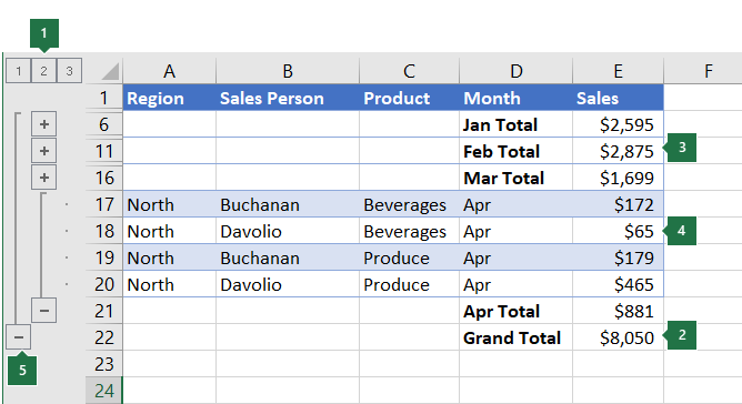
If you have a list of data you want to group and summarize, you can create an outline of up to eight levels. Each inner level, represented by a higher number in the outline symbols, displays detail data for the preceding outer level, represented by a lower number in the outline symbols. Use an outline to quickly display summary rows or columns, or to reveal the detail data for each group. You can create an outline of rows (as shown in the example below), an outline of columns, or an outline of both rows and columns.
|
|
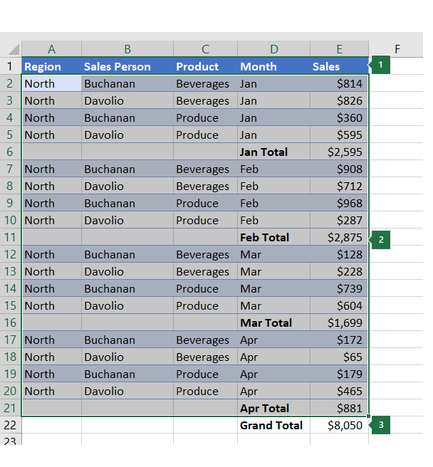
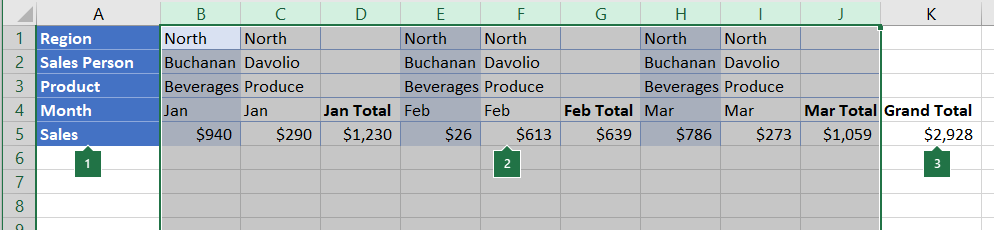
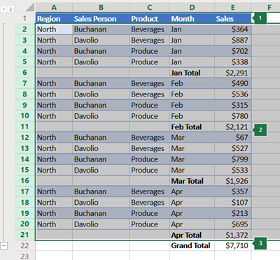
1. To display rows for a level, click the appropriate 2. Level 1 contains the total sales for all detail rows. 3. Level 2 contains total sales for each month in each region. 4. Level 3 contains detail rows — in this case, rows 17 through 20. 5. To expand or collapse data in your outline, click the |
 outline symbols.
 and
and  outline symbols, or press ALT+SHIFT+= to expand and ALT+SHIFT+- to collapse.
-
Make sure that each column of the data that you want to outline has a label in the first row (e.g., Region), contains similar facts in each column, and that the range you want to outline has no blank rows or columns.
-
If you want, your grouped detail rows can have a corresponding summary row—a subtotal. To create these, do one of the following:
-
Insert summary rows by using the Subtotal command
Use the Subtotal command, which inserts the SUBTOTAL function immediately below or above each group of detail rows and automatically creates the outline for you. For more information about using the Subtotal function, see SUBTOTAL function.
-
Insert your own summary rows
Insert your own summary rows, with formulas, immediately below or above each group of detail rows. For example, under (or above) the rows of sales data for March and April, use the SUM function to subtotal the sales for those months. The table later in this topic shows you an example of this.
-
-
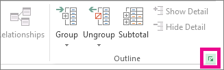
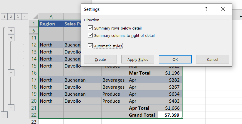
By default, Excel looks for summary rows below the details they summarize, but it’s possible to create them above the detail rows. If you created the summary rows below the details, skip to the next step (step 4). If you created your summary rows above your detail rows, on the Data tab, in the Outline group, click the dialog box launcher.

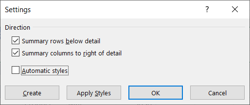
The Settings dialog box opens.
Then in the Settings dialog box, clear the Summary rows below detail checkbox, and then click OK.
-
Outline your data. Do one of the following:
Outline the data automatically
-
Select a cell in the range of cells you want to outline.
-
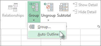
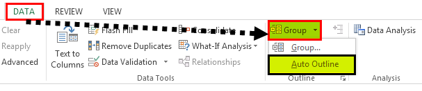
On the Data tab, in the Outline group, click the arrow under Group, and then click Auto Outline.
Outline the data manually
Important: When you manually group outline levels, it’s best to have all data displayed to avoid grouping the rows incorrectly.
-
To outline the outer group (level 1), select all of the rows the outer group will contain (i.e., the detail rows and if you added them, their summary rows).
1. The first row contains labels, and is not selected.
2. Since this is the outer group, select all the rows with subtotals and details.
3. Don’t select the grand total.
-
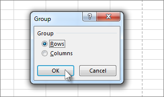
On the Data tab, in the Outline group, click Group. Then in the Group dialog box, click Rows, and then click OK.
Tip: If you select entire rows instead of just the cells, Excel automatically groups by row — the Group dialog box doesn’t even open.
The outline symbols appear beside the group on the screen.
-
Optionally, outline an inner, nested group — the detail rows for a given section of your data.
Note: If you don’t need to create any inner groups, skip to step f, below.
For each inner, nested group, select the detail rows adjacent to the row that contains the summary row.
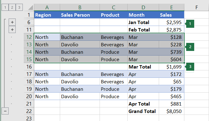
1. You can create multiple groups at each inner level. Here, two sections are already grouped at level 2.
2. This section is selected and ready to group.
3. Don’t select the summary row for the data you are grouping.
-
On the Data tab, in the Outline group, click Group.
Then in the Group dialog box, click Rows, and then click OK. The outline symbols appear beside the group on the screen.
Tip: If you select entire rows instead of just the cells, Excel automatically groups by row — the Group dialog box doesn’t even open.
-
Continue selecting and grouping inner rows until you have created all of the levels that you want in the outline.
-
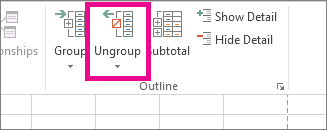
If you want to ungroup rows, select the rows, and then on the Data tab, in the Outline group, click Ungroup.
You can also ungroup sections of the outline without removing the entire level. Hold down SHIFT while you click the
or for the group, and then on the Data tab, in the Outline group, click Ungroup.Important: If you ungroup an outline while the detail data is hidden, the detail rows may remain hidden. To display the data, drag across the visible row numbers adjacent to the hidden rows. Then on the Home tab, in the Cells group, click Format, point to Hide & Unhide, and then click Unhide Rows.
-
-
Make sure that each row of the data that you want to outline has a label in the first column, contains similar facts in each row, and the range has no blank rows or columns.
-
Insert your own summary columns with formulas immediately to the right or left of each group of detail columns. The table listed in step 4 below shows you an example.
Note: To outline data by columns, you must have summary columns that contain formulas that reference cells in each of the detail columns for that group.
-
If your summary column is to the left of the detail columns, on the Data tab, in the Outline group, click the dialog box launcher.
The Settings dialog box opens.
Then in the Settings dialog box, clear the Summary columns to right of detail check box, and click OK.
-
To outline the data, do one of the following:
Outline the data automatically
-
Select a cell in the range.
-
On the Data tab, in the Outline group, click the arrow below Group and click Auto Outline.
Outline the data manually
Important: When you manually group outline levels, it’s best to have all data displayed to avoid grouping columns incorrectly.
-
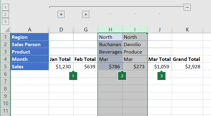
To outline the outer group (level 1), select all of the subordinate summary columns, as well as their related detail data.
1. Column A contains labels.
2. Select all the detail and subtotal columns. Note that if you don’t select entire columns, when you click Group (on the Data tab in the Outline group) the Group dialog box will open and ask you to choose Rows or Columns.
3. Don’t select the grand total column.
-
On the Data tab, in the Outline group, click Group.
The outline symbol appears above the group.
-
To outline an inner, nested group of detail columns (level 2 or higher), select the detail columns adjacent to the column that contains the summary column.
1. You can create multiple groups at each inner level. Here, two sections are already grouped at level 2.
2. These columns are selected and ready to group. Note that if you don’t select entire columns, when you click Group (on the Data tab in the Outline group) the Group dialog box will open and ask you to choose Rows or Columns.
3. Don’t select the summary column for the data you are grouping.
-
On the Data tab, in the Outline group, click Group.
The outline symbols appear beside the group on the screen.
-
-
Continue selecting and grouping inner columns until you have created all of the levels that you want in the outline.
-
If you want to ungroup columns, select the columns, and then on the Data tab, in the Outline group, click Ungroup.
You can also ungroup sections of the outline without removing the entire level. Hold down SHIFT while you click the  or
or  for the group, and then on the Data tab, in the Outline group, click Ungroup.
If you ungroup an outline while the detail data is hidden, the detail columns may remain hidden. To display the data, drag across the visible column letters adjacent to the hidden columns. On the Home tab, in the Cells group, click Format, point to Hide & Unhide, and then click Unhide Columns
-
If you don’t see the outline symbols
, , and , go to File > Options > Advanced, and then under the Display options for this worksheet section, select the Show outline symbols if an outline is applied check box, and then click OK. -
Do one or more of the following:
-
Show or hide the detail data for a group
To display the detail data within a group, click the
button for the group, or press ALT+SHIFT+=. -
To hide the detail data for a group, click the
button for the group, or press ALT+SHIFT+-. -
Expand or collapse the entire outline to a particular level
In the
outline symbols, click the number of the level that you want. Detail data at lower levels is then hidden.For example, if an outline has four levels, you can hide the fourth level while displaying the rest of the levels by clicking
. -
Show or hide all of the outlined detail data
To show all detail data, click the lowest level in the
outline symbols. For example, if there are three levels, click . -
To hide all detail data, click
.
-
 .
. .
.For outlined rows, Microsoft Excel uses styles such as RowLevel_1 and RowLevel_2 . For outlined columns, Excel uses styles such as ColLevel_1 and ColLevel_2. These styles use bold, italic, and other text formats to differentiate the summary rows or columns in your data. By changing the way each of these styles is defined, you can apply different text and cell formats to customize the appearance of your outline. You can apply a style to an outline either when you create the outline or after you create it.
Do one or more of the following:
Automatically apply a style to new summary rows or columns
-
On the Data tab, in the Outline group, click the dialog box launcher.
The Settings dialog box opens.
-
Select the Automatic styles check box.
Apply a style to an existing summary row or column
-
Select the cells to which you want to apply a style.
-
On the Data tab, in the Outline group, click the dialog box launcher.
The Settings dialog box opens.
-
Select the Automatic styles check box, and then click Apply Styles.
You can also use autoformats to format outlined data.
-
If you don’t see the outline symbols
, , and , go to File > Options > Advanced, and then under the Display options for this worksheet section, select the Show outline symbols if an outline is applied check box. -
Use the outline symbols
, , and to hide the detail data that you don’t want copied.For more information, see the section, Show or hide outlined data.
-
Select the range of summary rows.
-
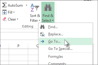
On the Home tab, in the Editing group, click Find & Select, and then click Go To.
-
Click Go To Special.
-
Click Visible cells only.
-
Click OK, and then copy the data.
Note: No data is deleted when you hide or remove an outline.
Hide an outline
-
Go to File > Options > Advanced, and then under the Display options for this worksheet section, uncheck the Show outline symbols if an outline is applied check box.
Remove an outline
-
Click the worksheet.
-
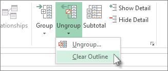
One the Data tab, in the Outline group, click Ungroup and click Clear Outline.
Important: If you remove an outline while the detail data is hidden, the detail rows or columns may remain hidden. To display the data, drag across the visible row numbers or column letters adjacent to the hidden rows and columns. On the Home tab, in the Cells group, click Format, point to Hide & Unhide, and then click Unhide Rows or Unhide Columns.
Imagine that you want to create a summary report of your data that only displays totals accompanied by a chart of those totals. In general, you can do the following:
-
Create a summary report
-
Outline your data.
For more information, see the sections Create an outline of rows or Create an outline of columns.
-
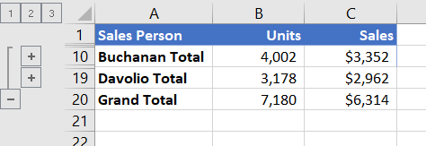
Hide the detail by clicking the outline symbols
, , and to show only the totals as shown in the following example of a row outline:
-
For more information, see the section, Show or hide outlined data.
-
-
Chart the summary report
-
Select the summary data that you want to chart.
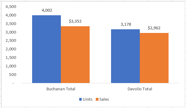
For example, to chart only the Buchanan and Davolio totals, but not the grand totals, select cells A1 through C19 as shown in the above example.
-
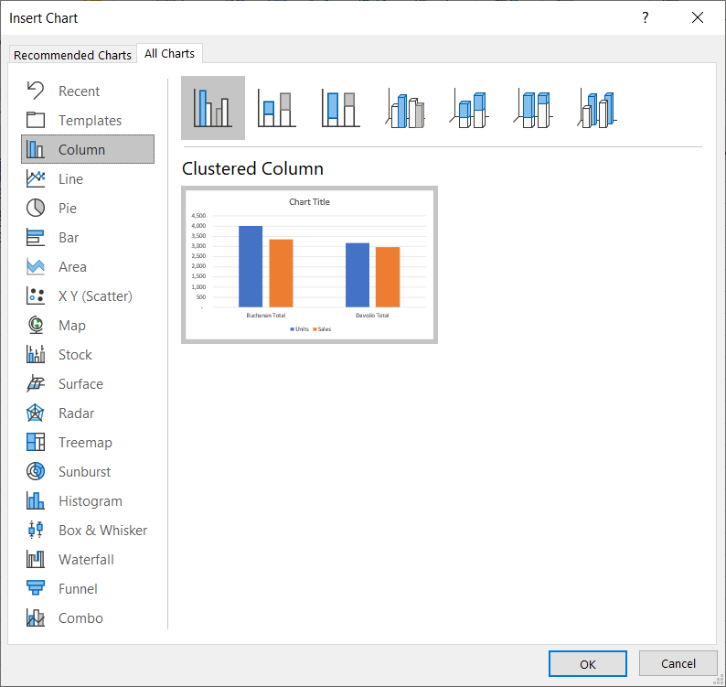
Click Insert > Charts > Recommended Charts, then click the All Charts tab and choose your chart type.
For example, if you chose the Clustered Column option, your chart would look like this:
If you show or hide details in the outlined list of data, the chart is also updated to show or hide the data.
-
You can group (or outline) rows and columns in Excel for the web.
Note: Although you can add summary rows or columns to your data (by using functions such as SUM or SUBTOTAL), you cannot apply styles or set a position for summary rows and columns in Excel for the web.
Create an outline of rows or columns
|
|
|
|
Outline of rows in Excel Online
|
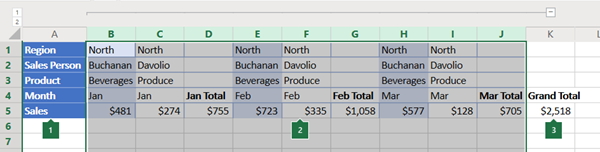
Outline of columns in Excel Online
|
-
Make sure that each column (or row) of the data that you want to outline has a label in the first row (or column), contains similar facts in each column (or row), and that the range has no blank rows or columns.
-
Select the data (including any summary rows or columns).
-
On the Data tab, in the Outline group, click Group > Group Rows or Group Columns.
-
Optionally, if you want to outline an inner, nested group — select the rows or columns within the outlined data range, and repeat step 3.
-
Continue selecting and grouping inner rows or columns until you have created all of the levels that you want in the outline.
Ungroup rows or columns
-
To ungroup, select the rows or columns, and then on the Data tab, in the Outline group, click Ungroup and select Ungroup Rows or Ungroup Columns.
Show or hide outlined data
Do one or more of the following:
Show or hide the detail data for a group
-
To display the detail data within a group, click the
for the group, or press ALT+SHIFT+=. -
To hide the detail data for a group, click the
for the group, or press ALT+SHIFT+-.
Expand or collapse the entire outline to a particular level
-
In the
outline symbols, click the number of the level that you want. Detail data at lower levels is then hidden. -
For example, if an outline has four levels, you can hide the fourth level while displaying the rest of the levels by clicking
.
Show or hide all of the outlined detail data
-
To show all detail data, click the lowest level in the
outline symbols. For example, if there are three levels, click . -
To hide all detail data, click
.
Need more help?
You can always ask an expert in the Excel Tech Community or get support in the Answers community.
See Also
Group or ungroup data in a PivotTable
What Is Group In Excel?
The Group is an Excel tool that groups two or more rows or columns. With this function, the user has the option to minimize and maximize the grouped data. The rows or columns of the group collapse on minimizing and expand on maximizing. The group option is available under the Outline section of the Data tab.
You are free to use this image on your website, templates, etc, Please provide us with an attribution linkArticle Link to be Hyperlinked
For eg:
Source: Group in Excel (wallstreetmojo.com)
Table of contents
- What is Group in Excel?
- How to Group Data in Excel?
- Auto Outline With Succeeding Subtotals
- Auto Outline With Preceding Subtotals
- The Collapse and Expansion of Grouped Data
- Manual Grouping
- Automatic Subtotals
- Frequently Asked Questions
- Recommended Articles
- How to Group Data in Excel?
- The Group in excel is used to group two or more rows or columns.
- We can collapse or expand the grouped data by minimizing and maximizing, respectively.
- The Excel shortcut keys to group data are Shift+Alt+Right Arrow. Similarly, the shortcut keys to ungroup the grouped data are Shift+Alt+Left Arrow.
- The “clear outline” option removes grouping from the worksheet.
- When we are using the “auto outline” option while grouping, the subtotals can either precede or succeed the grouped data.
- Alternatively, we can also use the shortcut keys Shift+Alt+Left Arrow.
How to Group Data in Excel?
Let us consider a few examples.
Example #1 – Auto Outline With Succeeding Subtotals
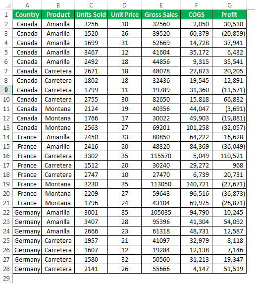
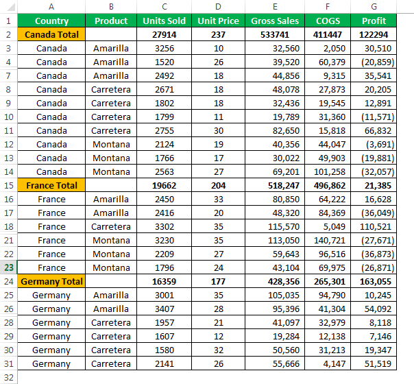
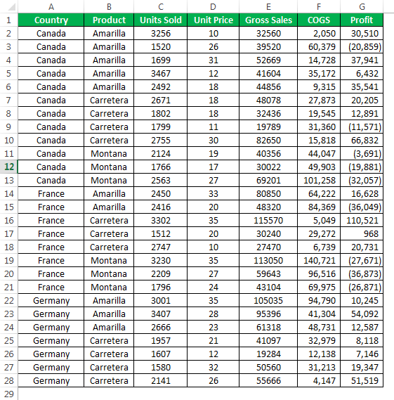
The Excel sheet consisting of the country name, product, units sold, price, gross sales, COGS, and profit is shown in the succeeding image. We can either club the countries into one or group the products into categories to make the data precise.
Let us go with the former approach and club the countries.
The steps to create an auto outline with succeeding subtotals are listed as follows:
- Enter the data as shown in the following image.

- To each country, add subtotals manually

- Place the cursor inside the table. Click on Auto outline in Group under the Data tab.

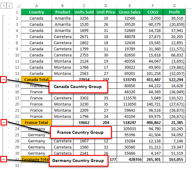
- Clicking on Auto Outline will group the range included in the country-wise total.

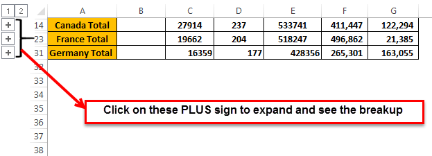
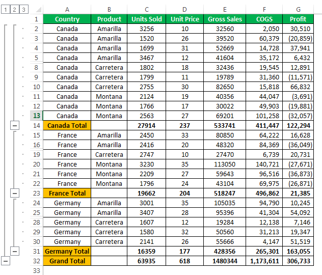
- Clicking the plus sign (+) hides the sub-items of each country. The consolidated summary of every country can be seen as highlighted in the below image.


Example #2 – Auto Outline With Preceding Subtotals
In the previous method, we added the totals at the end of every country. Let us add the totals before the data of a particular country.
The steps to group data with preceding totals are:
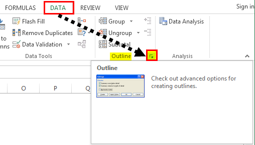
- Step 1: Click on the Dialog Box Launcher under the Outline section of the Data tab.
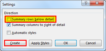
- Step 2: The Settings dialog box appears.
Uncheck the box Summary rows below detail and click on Create to complete the process.
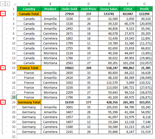
- Step 3: The group buttons appear at the top.
Example #3 – The Collapse And Expansion Of Grouped Data
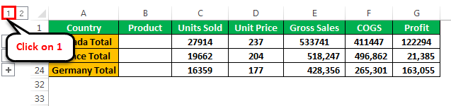
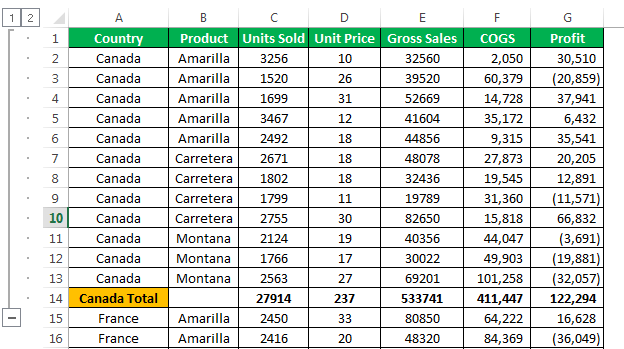
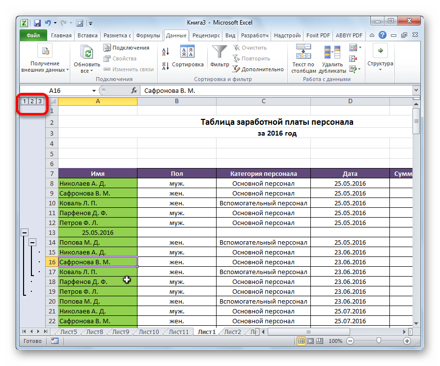
At any point in time, we can collapse or expand the group. In the top left-hand corner, there are two numbers following the name box. The numbers 1 and 2 appear within the boxes.
Clicking on 1 reveals the group summary, as shown in the following image.
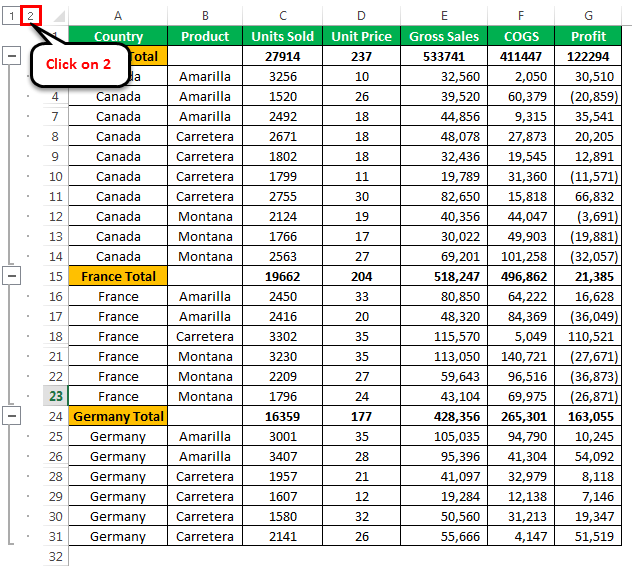
Clicking on 2 expands the table and reveals the breakup of the group, as shown below.
Example #4 – Manual Grouping
The previous examples utilize the basic Excel formulas and groups automatically. An alternative method is to group manually.
The steps for manual grouping are as follows:
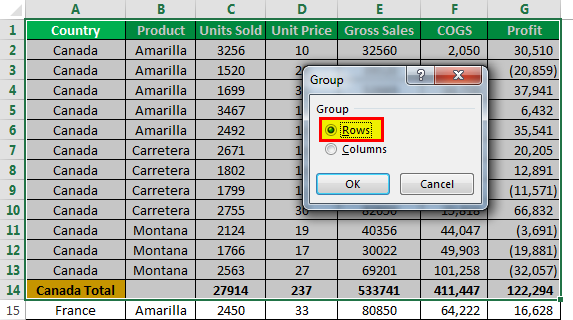
- Step 1: Select the range (row-wise) that we have to group. To group Canada, select the range till row 14.
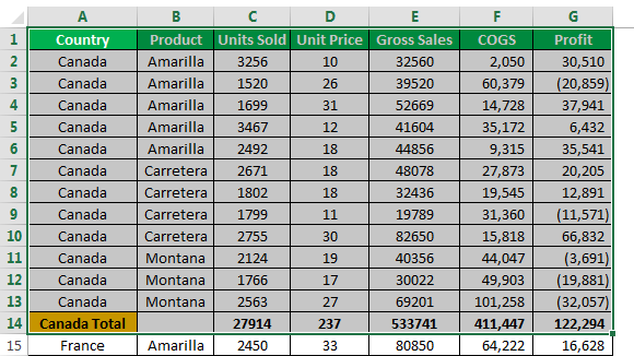
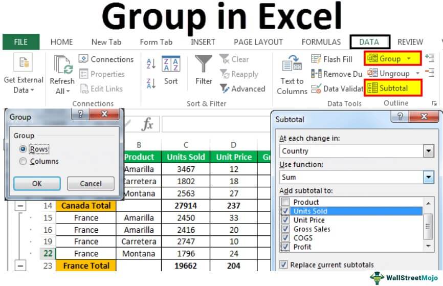
- Step 2: Select Group under the Data tab.
- Step 3: A dialog box, titled Group appears.
Since we are grouping the data row-wise, select “rows” option.
Alternatively, the Excel shortcut Shift+Alt+Right Arrow groups selected cells of the data.
- Step 4: Now, we have grouped the rows of Canada.
Remember, we have to repeat the process of manually grouping for the other countries as well. Please note that we should select the data of every country before grouping.
Note: The data should not contain any hidden rows during manual grouping.
Example #5 – Automatic Subtotals
In the previous examples, we added the subtotals manually. Alternatively, we can also add subtotals automatically.
The steps to add subtotals automatically are:
- Step 1: First, we should remove all the added subtotals manually.
- Step 2: Click on Subtotal under the Data tab.

- Step 3: The Subtotal dialog box appears.
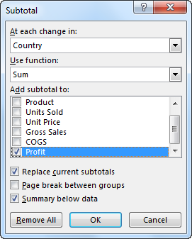
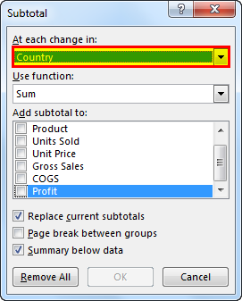
- Step 4: Select the basis on which subtotals are to be added.
- Select Country as the base, under At each change in: option.
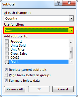
- Step 5: Since totals are required, select Sum under Use function: option.
Note: The user can select different functions like sum, average, min, max, etc., in the “subtotal” dialog box.
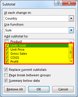
- Step 6: For totaling the columns, select them under Add subtotal to:. Check the boxes for Units Sold, unit price, Gross Sales, COGS, and Profit.
Click OK.
- Step 7: The subtotals and the groups appear, as shown below.
Important Things To Note
- Group in excel is used to group rows and columns.
- It is used to create structured financial models.
- Also, it helps to read complex data.
Frequently Asked Questions
1. What is group in Excel?
The Group in Excel is a tool that helps club similar data. It provides an organized, compact, and readable view to the reader. For grouping, the worksheet must contain headings and subtotals for every column and row respectively. Moreover, there should not be any blank cells in the data to be grouped.
The groups in Excel are used to create structured financial models. Since groups provide minimize and maximize options, they are used to hide unnecessary calculations.
2. Why is data grouped and ungrouped in Excel?
The data is grouped and ungrouped for the following reasons:
• Grouping helps read through the detailed and complex data. Ungrouping removes the grouping of rows and columns, thereby helping the user go back to the initial data view.
• With grouping, it is possible to look at the required data sections of the worksheet. Ungrouping helps to look at the entire worksheet data in one go.
Note: The grouping shortcut is Shift+Alt+Right Arrow, and the ungrouping shortcut is Shift+Alt+Left Arrow.
3. How does ungrouping work in Excel?
The ungrouping of data works as follows:
• To ungroup the entire data, clear the outline.
Click Clear outline under the Ungroup arrow (Outline section of the Data tab).
• To ungroup particular data, select the rows to be ungrouped. In the ungroup box, select Rows option and click OK.
Alternatively, we can also use the shortcut keys Shift+Alt+Left Arrow.
Note: Ungrouping does not delete any data. In case the outline is removed, it cannot be undone with Ctrl+Z.
Download Template
This article must be helpful to understand the Group in Excel, with its formula and examples. You can download the template here to use it instantly.
You can download this Group in Excel template here – Group in Excel template
Recommended Articles
This has been a guide to Group in Excel (Auto, Manual). Here we discuss how to group and ungroup data in Excel along with examples and downloadable Excel template. You may learn more about Excel from the following articles –
- Group Rows in Excel
- ExcelGroup Data
- Group Excel Worksheets
- Excel Column Grouping
Содержание
- Настройка группировки
- Группировка по строкам
- Группировка по столбцам
- Создание вложенных групп
- Разгруппирование
- Вопросы и ответы

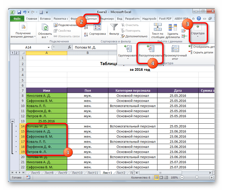
При работе с таблицами, в которые входит большое количество строк или столбцов, актуальным становится вопрос структурирования данных. В Экселе этого можно достичь путем использования группировки соответствующих элементов. Этот инструмент позволяет не только удобно структурировать данные, но и временно спрятать ненужные элементы, что позволяет сконцентрировать своё внимания на других частях таблицы. Давайте выясним, как произвести группировку в Экселе.
Настройка группировки
Прежде чем перейти к группировке строк или столбцов, нужно настроить этот инструмент так, чтобы конечный результат был близок к ожиданиям пользователя.
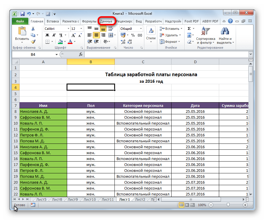
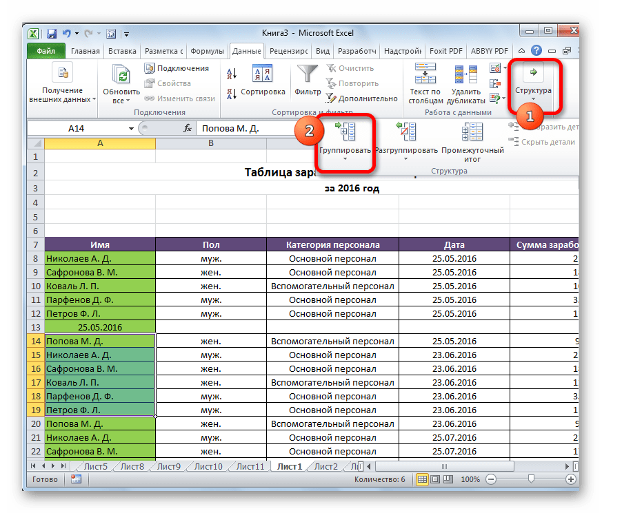
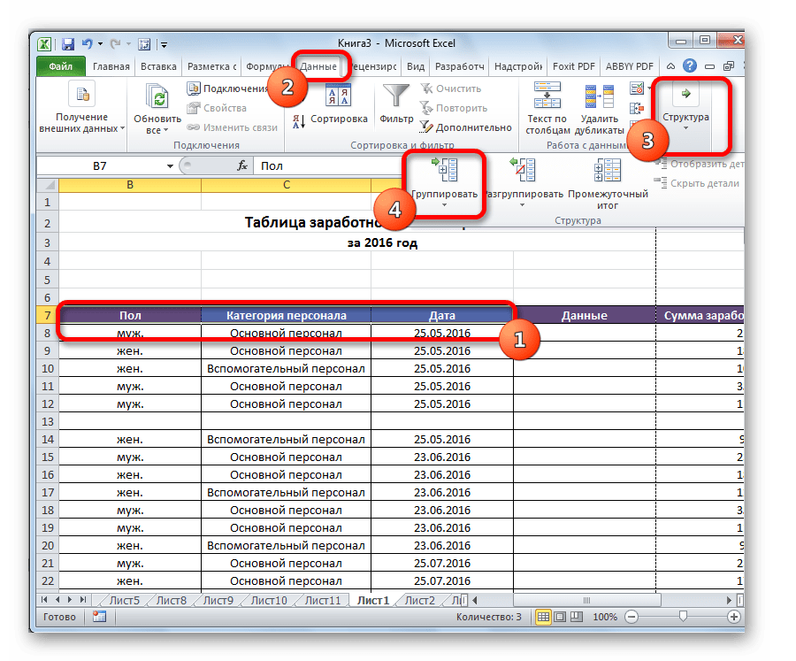
- Переходим во вкладку «Данные».
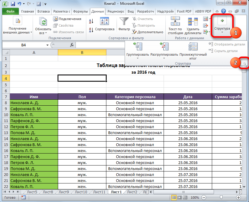
- В нижнем левом углу блока инструментов «Структура» на ленте расположена маленькая наклонная стрелочка. Кликаем по ней.
- Открывается окно настройки группировки. Как видим по умолчанию установлено, что итоги и наименования по столбцам располагаются справа от них, а по строкам – внизу. Многих пользователей это не устраивает, так как удобнее, когда наименование размещается сверху. Для этого нужно снять галочку с соответствующего пункта. В общем, каждый пользователь может настроить данные параметры под себя. Кроме того, тут же можно включить автоматические стили, установив галочку около данного наименования. После того, как настройки выставлены, кликаем по кнопке «OK».

На этом настройка параметров группировки в Эксель завершена.
Группировка по строкам
Выполним группировку данных по строкам.
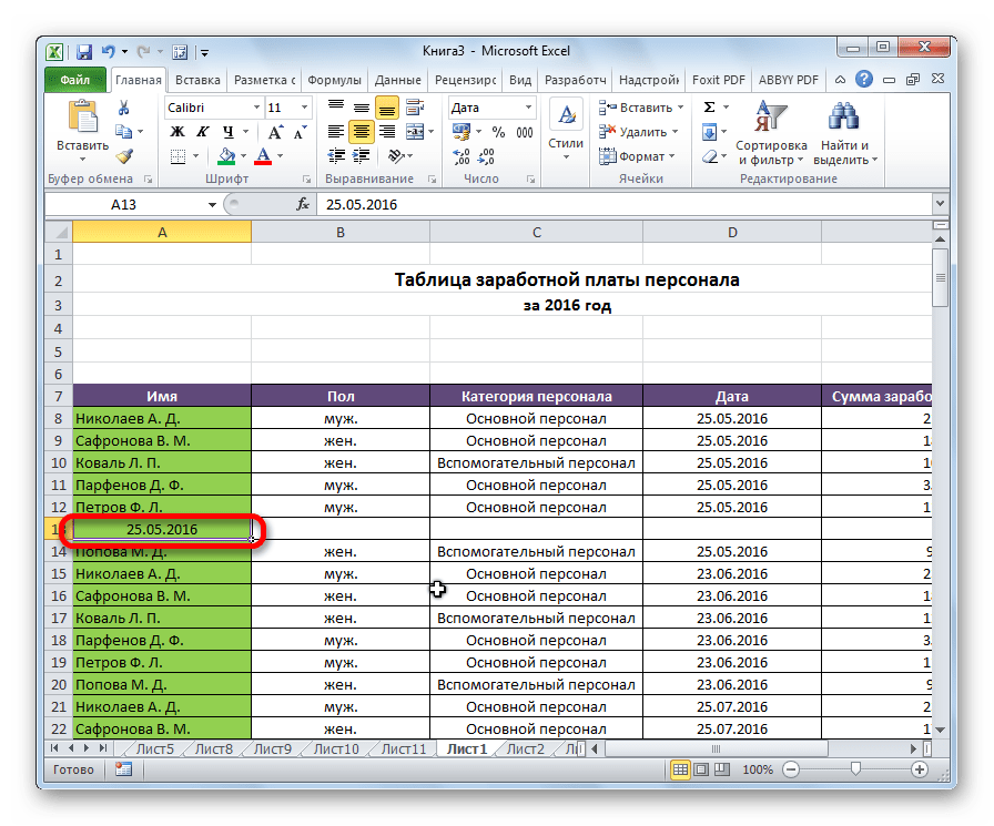
- Добавляем строчку над группой столбцов или под ней, в зависимости от того, как планируем выводить наименование и итоги. В новой ячейке вводим произвольное наименование группы, подходящее к ней по контексту.
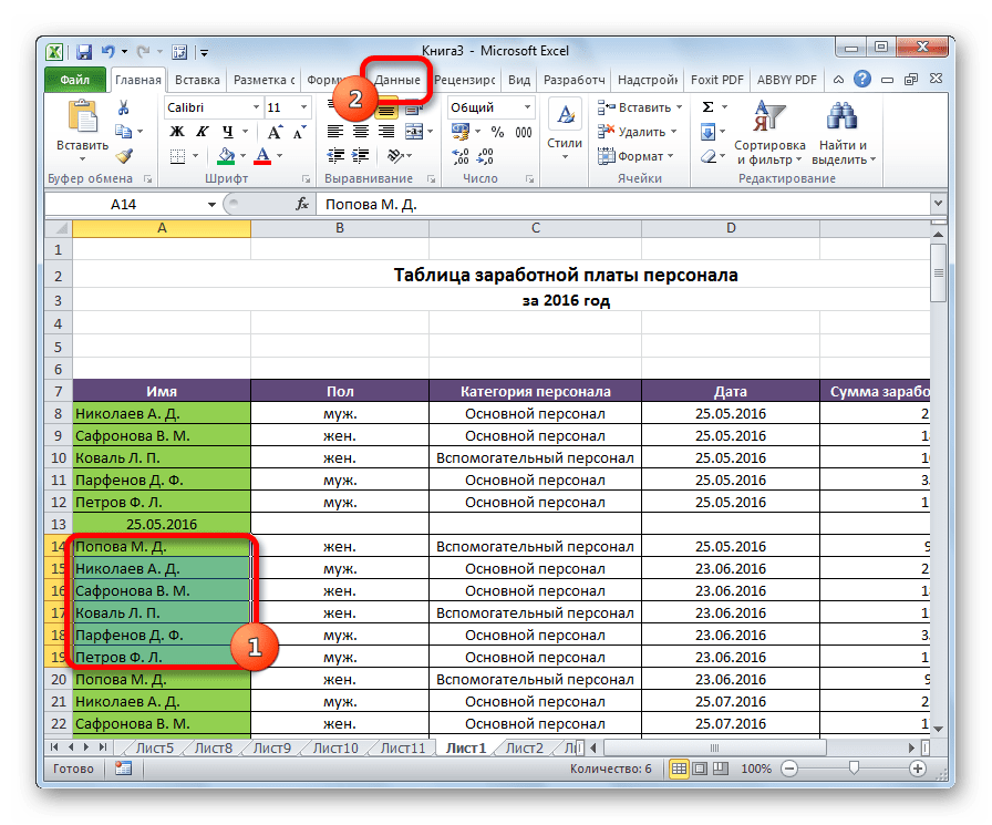
- Выделяем строки, которые нужно сгруппировать, кроме итоговой строки. Переходим во вкладку «Данные».
- На ленте в блоке инструментов «Структура» кликаем по кнопке «Группировать».
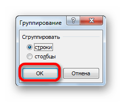
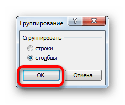
- Открывается небольшое окно, в котором нужно дать ответ, что мы хотим сгруппировать – строки или столбцы. Ставим переключатель в позицию «Строки» и жмем на кнопку «OK».
На этом создание группы завершено. Для того, чтобы свернуть её достаточно нажать на знак «минус».
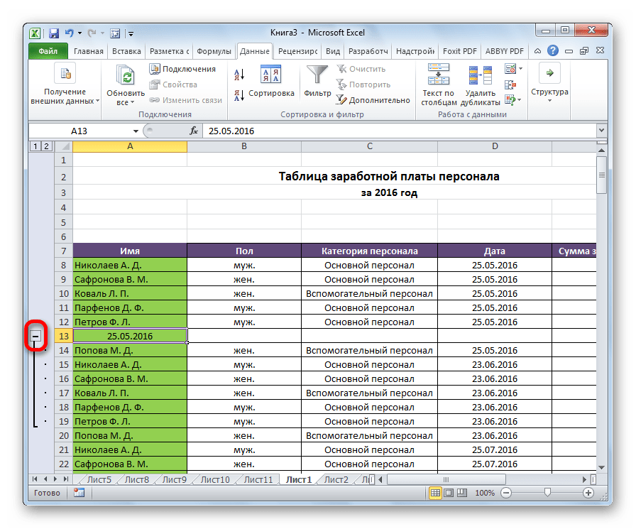
Чтобы заново развернуть группу, нужно нажать на знак «плюс».


Группировка по столбцам
Аналогичным образом проводится и группировка по столбцам.
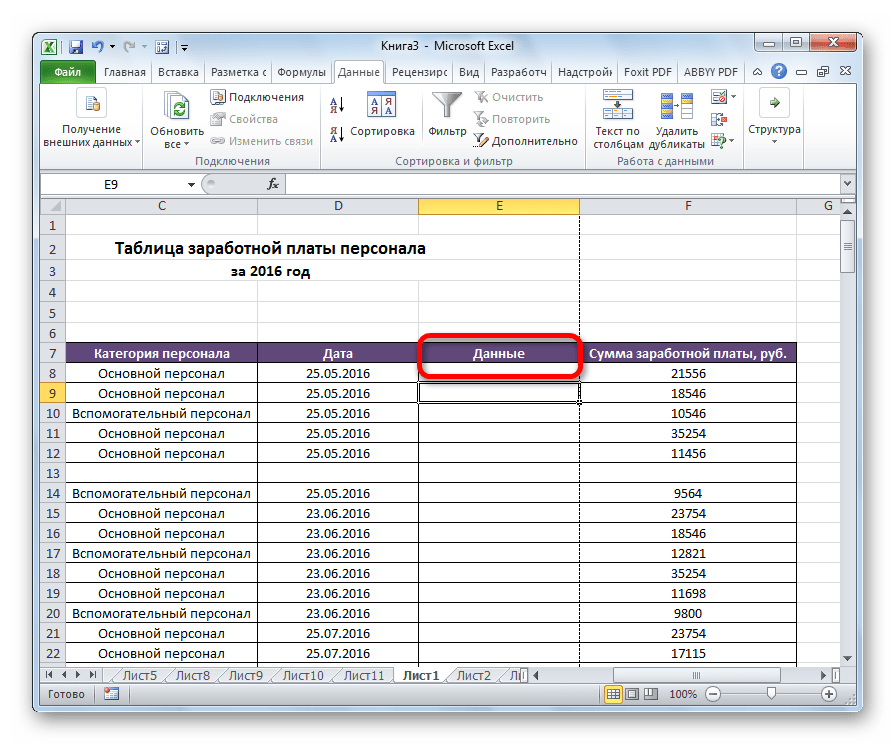
- Справа или слева от группируемых данных добавляем новый столбец и указываем в нём соответствующее наименование группы.
- Выделяем ячейки в столбцах, которые собираемся сгруппировать, кроме столбца с наименованием. Кликаем на кнопку «Группировать».
- В открывшемся окошке на этот раз ставим переключатель в позицию «Столбцы». Жмем на кнопку «OK».
Группа готова. Аналогично, как и при группировании столбцов, её можно сворачивать и разворачивать, нажимая на знаки «минус» и «плюс» соответственно.
Создание вложенных групп
В Эксель можно создавать не только группы первого порядка, но и вложенные. Для этого, нужно в развернутом состоянии материнской группы выделить в ней определенные ячейки, которые вы собираетесь сгруппировать отдельно. Затем следует провести одну из тех процедур, какие были описаны выше, в зависимости от того, со столбцами вы работаете или со строками.
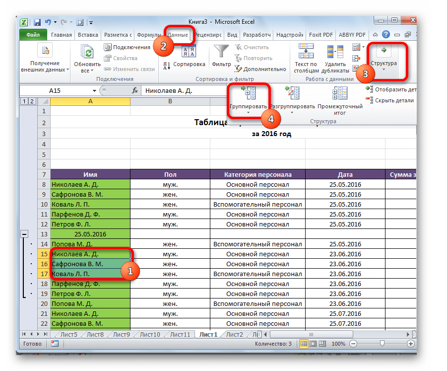
После этого вложенная группа будет готова. Можно создавать неограниченное количество подобных вложений. Навигацию между ними легко проводить, перемещаясь по цифрам, расположенным слева или сверху листа в зависимости от того, что сгруппировано строки или столбцы.
Разгруппирование
Если вы хотите переформатировать или просто удалить группу, то её нужно будет разгруппировать.
- Выделяем ячейки столбцов или строк, которые подлежат разгруппированию. Жмем на кнопку «Разгруппировать», расположенную на ленте в блоке настроек «Структура».
- В появившемся окошке выбираем, что именно нам нужно разъединить: строки или столбцы. После этого, жмем на кнопку «OK».

Теперь выделенные группы будут расформированы, а структура листа примет свой первоначальный вид.
Как видим, создать группу столбцов или строк довольно просто. В то же время, после проведения данной процедуры пользователь может значительно облегчить себе работу с таблицей, особенно если она сильно большая. В этом случае также может помочь создание вложенных групп. Провести разгруппирование так же просто, как и сгруппировать данные.
Еще статьи по данной теме:
Помогла ли Вам статья?
The best way to keep spreadsheets organized
Guide on How to Group in Excel
Grouping rows and columns in Excel[1] is critical for building and maintaining a well-organized and well-structured financial model. Using the Excel group function is the best practice when it comes to staying organized, as you should never hide cells in Excel. This guide will show you how to group in Excel with step-by-step instructions, examples, and screenshots.

Keyboard Shortcuts Sheet
Looking to be an Excel wizard? Increase your productivity with CFI’s comprehensive keyboard shortcuts guide.
Excel Group Function
The Excel group function is one of the best secrets a world-class financial analyst uses to make their work extremely organized and easy for other users of the spreadsheet to understand.
Reasons to use the Excel Group Function:
- To easily expand and contract sections of a worksheet
- To minimize schedules or side calculations that other users might not need
- To keep information organized
- As a substitute for creating new sheets (tabs)
- As a superior alternative to hiding cells
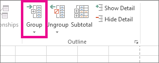
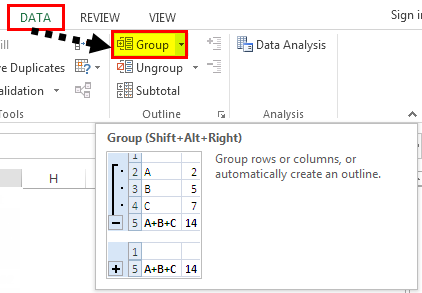
The function is found in the Data section of the Ribbon, then Group.
Example of How to Group in Excel
Let’s look at a simple exercise to see how it works. Suppose we have a schedule in a worksheet that is becoming quite long, and we want to reduce the amount of detail that’s shown. The screenshots below will show you how to properly implement grouping in Excel.
Here are the steps to follow to group rows:
- Select the rows you wish to add grouping to (entire rows, not just individual cells)
- Go to the Data Ribbon
- Select Group
- Select Group again
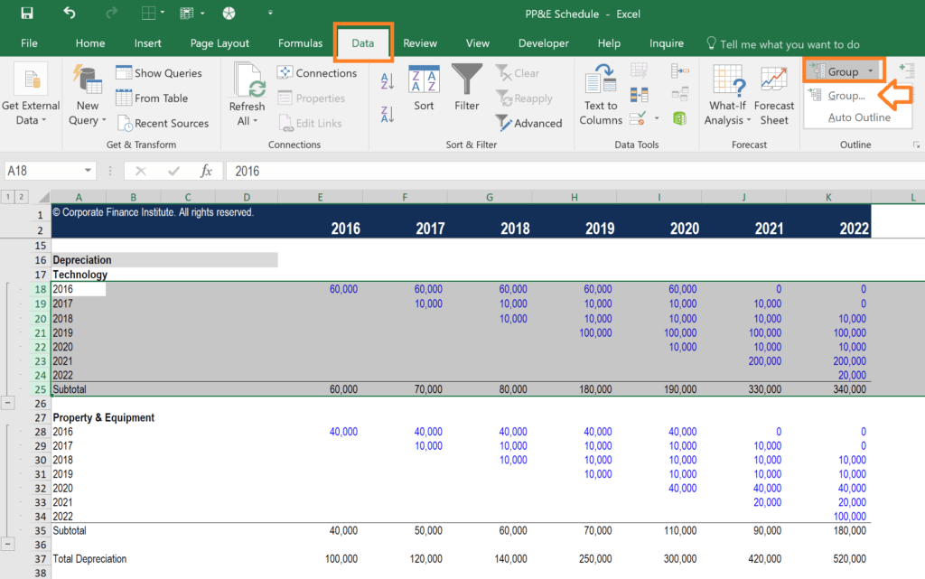
You can repeat the steps above as many times as you like, and you can also apply it to columns as well.
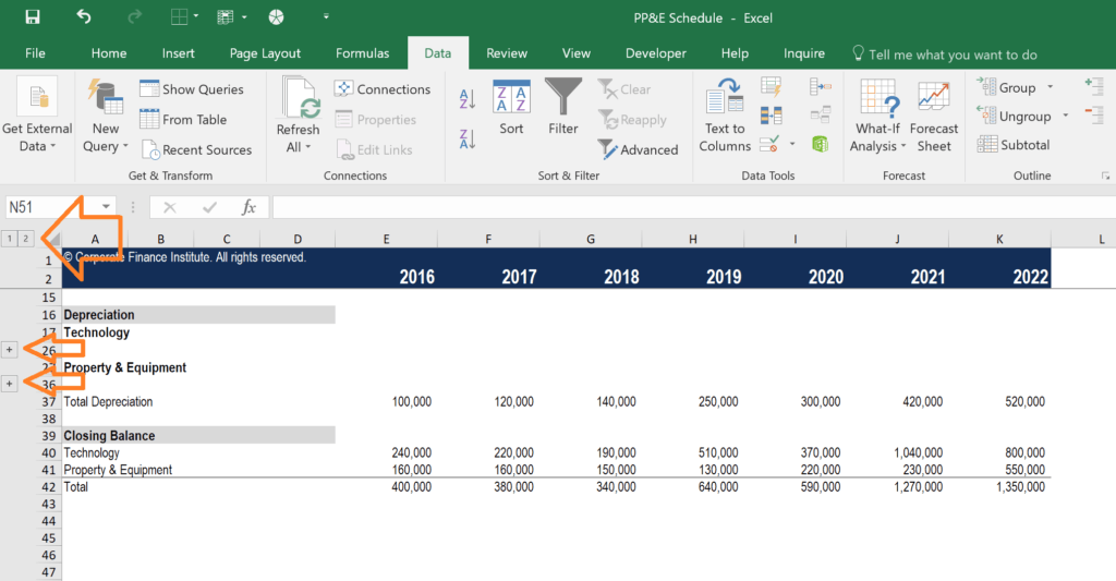
Once you’re finished, you can press the “-” buttons in the margin to collapse the rows or columns.
If you want to expand them again, press the “+” buttons in the margin, as shown in the screenshot below.
There is also a “1” button in the top left corner to collapse all groups, and a “2” button to expand all groups.
Why You Should Never Hide Cells in Excel
Though many people do it, you should never hide cells in Excel (or spreadsheets either, for that matter). The reason is that Excel does not make it clear to the user of the spreadsheet that cells have been hidden, and thus they may go unnoticed.
The only way to see that cells are hidden is to notice that the row number or column number suddenly jumps (e.g., from row 25 to row 167).
Since other users of the spreadsheet may not notice this (and you may forget yourself) you should never hide cells in Excel.
Download Excel Group Template
You can download the Template for free if you wish to use it as an example or starting point for how to group in Excel and apply it to your own work and financial analysis.
Additional Resources
Thank you for reading CFI’s guide to Group in Excel. To continue learning and advancing your career, these additional CFI resources will be helpful:
- List of 300+ Excel Functions
- Keyboard Shortcuts
- What is Financial Modeling?
- Financial Modeling Courses
- See all Excel resources
![]()
Download Article
Layer your data to stay organized
![]()
Download Article
- Preparing Your Data
- Outlining Automatically
- Outlining Manually
- Minimizing & Clearing
- Q&A
- Tips
- Warnings
|
|
|
|
|
|
Outlining (grouping) data in Excel is a great way to organize and summarize data. This feature nests your information into up to eight levels. Inner levels have the detailed data for the surrounding outer level. As long as your data has column headings and no blank rows, you can automatically group and outline automatically with Excel. This wikiHow guide teaches you how to group and outline Excel data so you can work with large data sets more efficiently.
This works on Windows and Mac!
Things You Should Know
- Prepare your data by making column or row headers and getting rid of blank rows and columns.
- Outline rows or columns automatically by selecting a cell in the data and going to Data > Group > Auto Outline.
- For the manual method, click the Group button and choose “Rows” or “Columns.”
-
1
Organize the data you want to outline. Each column should have a column header in the first row. Make sure the range you’re going to outline doesn’t contain blank rows or columns.[1]
- For a general spreadsheet guide, check out how to make a spreadsheet in Excel and format it.
- If you’re looking for Excel database info, read our guide on creating a database from an Excel spreadsheet.
- Are you using the free version of Excel and considering upgrading to Microsoft 365? See our coupon site for Staples discounts.
-
2
Optionally, create a summary row. This is also called a subtotal. You have two options for this:
- Select a cell in the data range. Go to the Data tab and click Subtotal in the Outline group.
- Insert summary rows with your own formulas. For example, you could use the SUM function to subtotal information. These can go above or below the data.
- If you place your summary rows above the data, open the dialog box in the Outline group of the Data tab (it’s the right angle with an arrow). Uncheck “Summary rows below detail.”


Advertisement
-
1
Select a cell that’s in the range you’re going to outline. This can be any cell in the data.
- Your data must have column headers and no blank lines for this feature to work.
-
2
Click the Data tab. It’s on the left side of the green ribbon that’s at the top of the Excel window. Doing so will open a toolbar below the ribbon.
-
3
Click the down arrow under the Group button. You’ll find this option on the far-right side of the Data tab. A drop-down menu will appear.
-
4
Click Auto Outline. It’s in the Group drop-down menu.
- If you receive a pop-up box that says «Cannot create an outline», your data doesn’t have an outline-compatible formula in it. You may also have some blank cells in your data or missing column headers. You’ll need to manually outline the data.


Advertisement
-
1
Select your data. Click and drag your cursor from the top-left cell of the data you want to group to the bottom-right cell of the data.
-
2
Click Data if this tab isn’t open. It’s in the left side of the green ribbon at the top of Excel.
-
3
Click Group. It’s on the right side of the Data toolbar.
-
4
Select a group option. Click Rows to minimize your data vertically, or click Columns to minimize horizontally.
-
5
Click OK. It’s at the bottom of the pop-up window. Your grouped data is all set!


Advertisement
-
1
Minimize your data. Click the [-] button at the top or on the left side of the Excel spreadsheet to hide the grouped data. In most cases, doing this will only display the final line of the data.
-
2
Clear your outline if needed. Click Ungroup to the right of the Group option, then click Clear Outline… in the drop-down menu. This will ungroup and unhide any data that was minimized or grouped previously.


Advertisement
Add New Question
-
Question
How do I reverse the grouping so that the total is at the top line and the collapsed lines fall below?

Click the «Data» tab, then come to the «Outline» section, then click the small arrow on the right bottom corner to «Show the Outline Dialog Box». From the settings, unclick «Summary Rows Below Detail.»
-
Question
My data is grouped, but I cannot see the outline symbols along the left side of my spreadsheet. What can I do?
While the document is open, go to «File,» «Options,» «Advanced,» «Display options for this worksheet.» Make sure «Show outline symbols if an outline is applied» is selected. This is necessary for every sheet where there are outlines/groupings applied.
-
Question
How do I group Rows 23 through 31 and then group Rows 32 through 36? When I do it, Excel groups Rows 23 thru 36.
You need an empty row between your two groups. Otherwise Excel will automatically merge them.
See more answers
Ask a Question
200 characters left
Include your email address to get a message when this question is answered.
Submit
Advertisement
-
You cannot use this function if the sheet is shared.
Thanks for submitting a tip for review!
Advertisement
-
Don’t use grouping/outlining if you plan to protect the worksheet. If you do, other users won’t be able to expand and collapse the rows.
Advertisement
About This Article
Article SummaryX
1. Open the Excel document.
2. Click Data
3. Click Group
4. Click Auto Outline
5. Click [-] to minimize data.
Did this summary help you?
Thanks to all authors for creating a page that has been read 1,502,512 times.