Group dates in excel

The ability to quickly group dates in Pivot Tables in Excel can be quite useful.

It helps you analyze data by getting different views by dates, weeks, months, quarters, and years.

For example, if you have credit card data, you may want to group it in different ways (such as grouping by months or quarters or years).

Similarly, if you have a call center data, then you may want to group it by minutes or hours.

Watch Video – Grouping Dates in Pivot Tables (Grouping by Months/Years)

How to Group Dates in Pivot Tables in Excel

Suppose you have a dataset as shown below:

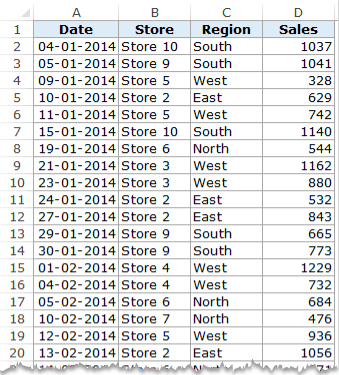
It has sales data by Date, Stores, and Regions (East, West, North, and South). The data spans across 300+ rows and 4 columns.

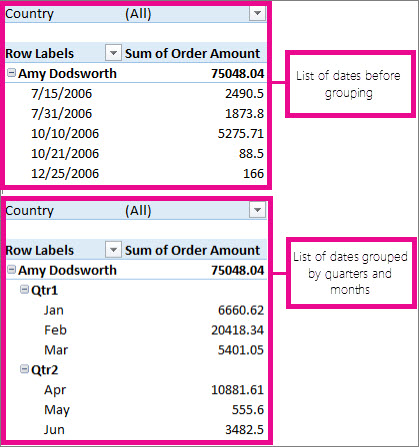
Here is a simple pivot table summary created using this data:

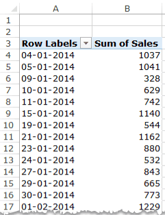
This pivot table summarizes sales data by date, but it isn’t quite helpful as it shows all the 300+ dates. In such as case, it would be better to have the dates grouped by years, quarters, and/or months

Download Data and follow along.

Grouping by Years in a Pivot Table

The dataset shown above have dates for two years (2014 and 2015).

Here are the steps to group these dates by years:

This would summarize the pivot table by years.

This summarization by years may be useful when you have more number of years. In this case, it would be better to have the quarterly or monthly data.

Grouping by Quarters in a Pivot Table

In the above dataset, it makes more sense to drill down to quarters or months to have a better understanding of the sales.

Here is how you can group these by quarters:

This would summarize the pivot table by quarters.

The issue with this pivot table is that it combines the Quarterly sales value for 2014 as well as 2015. Hence, for each quarter, the sales value is the sum of sales values in Quarter 1 in 2014 and 2015.

In a real life scenario, you are most likely to analyze these quarters for each year separately. To do this:

This would summarize the data by Years and then within years by Quarters. Something as shown below:

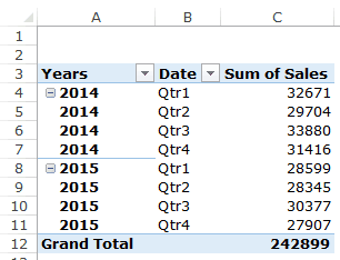
Note: I am using the tabular form layout in the above snapshot.

When you group dates by more than one time-frame group, something interesting happens. If you look at the field list, you will notice a new field has automatically been added. In this case, it is Years.

Note that this new field that has appeared is not a part of the data source. This field has been created in the Pivot Cache to quickly group and summarizes data. When you ungroup the data, this field will vanish.

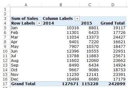
The benefit of having this new field is that now you can analyze the data with quarters in rows and years in columns, as shown below:

All you need to do is drop the Year field from Row area to Columns area.

Grouping by Months in a Pivot Table

Similar to the way we grouped the data by quarters, we can also do this by months.

Again, it is advisable to use both Year and Month to group the data instead of only using months (unless you only have data for one or less than a year).

Here are the steps to do this:

• Select any cell in the Date column in the Pivot Table.
• Go to Pivot Table Tools –> Analyze –> Group –> Group Selection.
• In the Grouping dialogue box, select Months as well as Years. You can select more than one option by simply clicking on it.
• Click OK.

This would group the date field and summarize the data as shown below:

Again, this would lead to a new field of Years getting added to the PivotTable fields. You can simply drag the years’ field to the columns area to get the years in columns and months is rows. You will get something as shown below:

Grouping by Weeks in a Pivot Table

While analyzing data such as store sales or website traffic, it makes sense to analyze it on a weekly basis.

When working with dates in Pivot Tables, grouping dates by week is a bit different than grouping by months, quarters, or years.

Here is how you can group dates by weeks:

• Select any cell in the Date column in the Pivot Table.
• Go to Pivot Table Tools –> Analyze –> Group –> Group Selection.
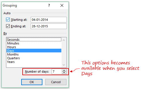
• In the Grouping dialogue box, select Days and deselect any other selected option(s). As soon as you do this, you would notice that the Number of Days option (at the bottom right) becomes available.
  • There is no inbuilt option to group by weeks. You need to group by days and specify the number of days to be used while grouping.
  • Note that for this to work, you need to select Days option only.
• In Number of days, enter 7 (or use the spin button to make the change).
• If you click OK at this point, your data would be grouped by weeks starting with January 4, 2014 – which is a Saturday. So the grouping would be from Saturday to Friday every week. To change this grouping and to begin the week from Monday, you need to change the start date (by default it picks the start date from the source data).
  • In such a case, you can either start the date on December 30, 2013, or January 6, 2014 (both Mondays).
• Click OK.

This will group the dates by weeks as shown below:

Similarly, you can group dates by specifying any other number of days. For example, instead of weekly, you can group dates in a biweekly interval.

Note:

• When you group dates by using this method, you can not group it using any other option (such as months, quarters or years).
• Calculated field/item would not work when you group using Days.

Grouping by Seconds/Hours/Minutes in a Pivot Table

If you working with high volumes of data (such as call center data), you may want to group it by seconds or minutes or hours.

You can use the same process to group the data by seconds, minutes, or hours.

Suppose you have the call center data as shown below:

In the above data, the date is recorded along with the time. In this case, it may make sense for the call center manager to analyze how the call resolve numbers are changing per hour.

Here is how to group the days by Hours:

This will group the data by hours and you will get something as shown below:

You can see that the Row Labels here are 09, 10, and so on.. which are the hours in a day. 09 would mean 9 AM and 18 would be 6 PM. Using this pivot table, you can easily identify that most calls are resolved during 1-2 PM.

Similarly, you can also group the dates on seconds and minutes.

How to Ungroup Dates in a Pivot Table in Excel

To ungroup dates in pivot tables:

• Select any cell in the date cells in the pivot table.
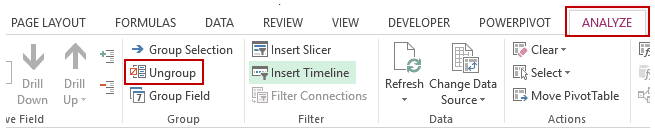
• Go to PivotTable Tools –> Analyze –> Group –> Ungroup.

This would instantly ungroup any grouping that you have done.

Download the Example File. 

Other Pivot Table Tutorials You May Like:

• Creating a Pivot Table in Excel – A Step by Step Tutorial.
• Preparing Source Data For Pivot Table.
• How to Group Numbers in Pivot Table in Excel.
• How to Filter Data in a Pivot Table in Excel.
• How to Apply Conditional Formatting in a Pivot Table in Excel.
• How to Refresh Pivot Table in Excel.
• How to Add and Use an Excel Pivot Table Calculated Field.
• Using Slicers in Excel Pivot Table.
• How to Replace Blank Cells with Zeros in Excel Pivot Tables.
• Count Distinct Values in Pivot Table

Before I was a Pivot Table guru, I had to get individual rows of daily sales and group them into a report showing the monthly sales during the year.

Group Dates in Pivot Table would take a ton of effort using Formulas:

• Extracting the month and year from each transactional date;
• Then manually grouping them together to get the total sales numbers for each month.  PAINFUL & SLOW!

Thankfully there is the Pivot Table way (I wish I had known this back then), which is quick and reduces the risks of making any errors….ah yeah & I almost forgot, it is also easy to add new data to your sales report with a simple Refresh!

In this article, we will be covering the following topics in detail:

• Group Dates in Pivot Table by Month & Year
• Group Dates in Pivot Table by Week
• Summarize Value by
• Change Formatting
• Control Automatic Grouping

Let’s look at each one of these!

Group Dates in Pivot Table by Month & Year

In the data below, you can see that there are two columns: one that contains the transaction date of the sale, and the second column contains the total sales amount for a particular date.

Want to know How To Group Dates in Pivot Table by Month?

In the example below, I show you how to Pivot Table Group by Month:

STEP 1: Insert a new Pivot table by clicking on your data and going to Insert > Pivot Table > New Worksheet or Existing Worksheet

STEP 2: In the ROWS section put in the Order Date field.

Notice that in Excel 2016 (the version that I am using) it will automatically Group the Order Date into Years & Quarters:

STEP 3: Right-click on any row in your Pivot Table and select Group so we can select our Group order that we want:

STEP 4: We need to deselect Quarters and make sure only Months and Years are selected (which will be highlighted in blue).

This will group our dates by the Months and Years.  Click OK.

STEP 5: In the VALUES area put in the Sales field.  This will get the total of the Sales for each Month & Year:

This is how you can easily create Pivot Table Group Dates by Month!

Your final grouped data is ready!

Change Formatting

Summarize Value by

In the previous examples, you saw how to get total sales by month, year, or week. You can even calculate the total number of sales that occurred in a particular month, year, or week.

Let’s look at an example to know how:

STEP 1: Right-click anywhere on the Pivot Table.

STEP 2: Select Value Field Settings from the list.

STEP 3: In the Value Field Setting dialog box, select Count.

STEP 4: Click OK.

This will summarize the values as a count of sales instead of the sum of sales (like before).

Ungroup Dates

To ungroup dates in a Pivot Table, simply right-click on the dates column and select ungroup.

Or, you can go to the PivotTable Analyze tab and select Ungroup.

Once this is done, the data will be ungrouped again.

Control Automatic Grouping

If you wish to, you can easily turn off this automatic date grouping feature in Excel 2016. To do that, follow the steps below:

STEP 1: Go to File Tab > Options

STEP 2: In the Excel Options dialog box, click Data in the categories on the left.

STEP 3: Check Disable automatic grouping of Date/Time columns in PivotTables checkbox.

STEP 4: Click OK.

This will easily turn off the automatic grouping feature in the Pivot Table! So, the date will be not be grouped automatically now when you drag the date field to an area in the pivot table.

Conclusion

You can easily analyze data by week, month, year, days, hour, etc., and find trends using this grouping dates feature in Pivot Table. It is a fairly simple and super quick method to group dates.

Did you know there are many creative ways of doing grouping in Excel Pivot Tables?

Learn all about it here!

About The Author

Home / Pivot Table / How to Group Dates in a Pivot Table

By grouping dates in a pivot table, you can create instant reports.

Here’s the point: Let’s say you want to group all the dates as months instead of adding a different column in your data, it’s better to group dates.

It’s super easy. Now here’s the good news: Apart from months, you can use years, quarters, time, and even a custom date range for grouping. And today in this post, I’d like to show you the exact steps for this.

Pivot Tables are one of the INTERMEDIATE EXCEL SKILLS.

Groups Dates in a Pivot Table by Month

Below are the steps you need to follow to group dates in a pivot table.

1. Select any of the cells from the date column.
2. Right-click on it and select group.
3. You will get a pop-up window to group dates.
4. Select “Month” in the group by option and then click OK.

You can also use the above steps to group dates in a pivot table by years, quarters, and days.

Weekly Summary

You can also create a group of 7 days to get a week-wise summary. Please follow the below steps to this.

1. Select “days” option from the group by option.
2. Enter 7 in a number of days.
   
3. Click OK.

You can use the above steps to create a group of dates for any number of days and please note that the week created by the pivot table is not on the basis of Mon-Sun.

Hourly Summary

You also have an option to group dates by time period. Let’s say if you have dates with time and you want to get an hourly summary. Just follow these simple steps for this.

1. Select any of the cells with a date.
2. Right click on it and select group.
3. Select hour from the group by option.
   
4. Click OK.
   

You can also use above steps to group dates in the pivot table by minutes and seconds.

Custom Date Range Summary

In the below pivot table, you have dates ranging from 01-Oct-2014 to 31-Jun-2015.

And you want to create a group of dates by month, but only for 6 months of 2015 and all the months of 2014 in one group. Well, you can also create a group of dates by using a custom range, follow these simple steps for this.

1. Right-click on date column and select “group”.
2. Untick starting and ending date in auto option. And, enter your custom dates.
3. Select month from by group option.
   
4. In the end, click OK.
   

In above pivot, now you have dates in a group by months for the date range you have mentioned and rest of the dates which are not in the date range are in a single category.

Related: Excel Slicer

Group Two Different Fields

It happens sometimes that you need to use more than one time span to group dates in a pivot table. Let’s suppose, in the below pivot table, you want to group dates by quarters and months.

1. First of all, select the group option from the right menu.
2. After that, select quarters and months.
3. In the end, click OK.

Once you create more than one group for dates in the pivot table, you will also get an expanding and collapsing option.

Un-Grouping

If you want to get back your dates or want to ungroup dates you can do that with the “ungroup‘ option.

1. Select a cell from the data column.
2. Right-click.
3. Select “Un-Group”.

Sample File

download

Group Dates in an Excel Pivot Table by Month and Year

by Avantix Learning Team | Updated March 7, 2021

Applies to: Microsoft^® Excel^® 2013, 2016, 2019 and 365 (Windows)

If you have valid dates entered in your source data, you can group by month, year or other date period in a pivot table in Excel. There are two common approaches to grouping by date. You can group by date periods in a pivot table using the Grouping feature (this may occur automatically depending on your version of Excel). Alternatively, you can also create calculations in source data to extract the month name and the year from a date field and use the fields in your pivot table.

Recommended article: How to Delete Blank Rows in Excel Worksheets (Great Strategies, Tricks and Shortcuts)

Do you want to learn more about Excel? Check out our virtual classroom or live classroom Excel courses >

Source data is typically entered vertically with data in columns and field names at the top of each column of data.

Grouping by month and year in a pivot table

The key to grouping by month and/or year in a pivot table is a source field with valid dates (such as OrderDate). Depending on your Control Panel settings on your device, valid dates may be entered as month/day/year, day/month/year or year/month/day (although they can be formatted to appear in other ways).

In Excel 2016 and later versions, if you drag a date field into the Rows or Columns area of a pivot table, Excel will group by date increments by default.

The easiest way to group by a date period is to right-click in a cell in a date field in a pivot table and select the desired grouping increments. You can group dates by quarters, years, months and days. The source data does not need to contain a year, quarter or month name column.

To group by month and/or year in a pivot table:

1. Click in a pivot table.
2. Drag a date field into the Row or Columns area in the PivotTable Fields task pane.
3. Select a date field cell in the pivot table that you want to group. Excel may have created a Year and/or Month field automatically.
4. Right-click the cell and select Group from the drop-down menu. You can also right-click a date field in the Rows or Columns area in the PivotTable Fields task pane. A dialog box appears.
5. Click the date periods that you want to group by. Select Quarters, Years, Months or Days. You can click on more than one such as Years and Months.
6. Click OK.

The Grouping dialog box offers multiple options for grouping by date:

The date field will be grouped and new fields will be added to the field list for the groups (if they didn’t exist beforehand).

In the following example, Excel grouped automatically by date periods in the PivotTable Fields task pane. This occurs in 2016 or later versions:

To remove a grouping period for a date field:

1. Select a date field cell in the pivot table that has been grouped.
2. Right-click the cell and select Group. You can also right-click a date field in the Rows or Columns area in the PivotTable Fields task pane. A dialog box appears.
3. Deselect or click the groups you wish to remove.
4. Click OK.

To remove all grouping:

1. Select a date field cell in the pivot table that has been grouped.
2. Right-click the cell and select Ungroup.

Controlling automatic grouping

In Excel 2016 and later versions, dates are grouped automatically if they are placed in the Rows or Columns area of the pivot table. You can turn this setting off or on.

To disable automatic grouping for pivot tables:

1. Click the File tab in the Ribbon.
2. Click Options. A dialog box appears.
3. Click Data in the categories on the left. If you are using an older version of Excel, click Advanced in the categories on the left.
4. Select or check Disable automatic grouping of Date/Time columns in PivotTables checkbox.
5. Click OK.

Below is the Excel Options dialog box in 365:

If you disable automatic grouping, you can still right-click and group in pivot tables but the groups will not be created automatically when you drag a date field to an area in the pivot table.

Issues with pivot table cache

When you create a pivot table and group using the Group feature, the fields and the groupings are stored in a pivot cache, not in the source data. This can be problematic if you create more pivot tables based on the same pivot cache. This means that all pivot tables that share the same cache, will also share the date groupings.

There is no easy way to see which pivot tables share the same cache in the Excel. You would need to use VBA (Visual Basic for Applications) to find this information.

You can unshare the cache by changing the source data range, but this can be tricky if you have a lot of pivot tables.

Creating date period fields in the source data

Another option is to create fields in the source data that calculate date periods (such as Year and Month). You can use the YEAR and TEXT functions to extract Year and Month from a valid date field.

For example, if you have a date in column A, you could create a calculation to extract the Year in column B and the Month in column C.

To calculate the year in B2 (assuming there is a valid date in A2), enter the following formula and then copy the formula down:

=YEAR(A2)

To calculate the month name in C2 (assuming there is a valid date in A2), enter the following formula and then copy the formula down:

=TEXT(A2,»mmmm»)

If the source data is in an Excel table, it’s best to use structured referencing formulas in each row such as =YEAR([@OrderDate]) or =TEXT([@OrderDate],»mmmm») where OrderDate is the name of the field and @ is a specifier to refer to the current row or record.

The benefit of creating the fields in the source data is that you can create a pivot table and then group by these fields in the pivot table simply by dragging them into the Rows or Columns area. You will be able to create other pivot tables that do not include the date grouping.

Another advantage of creating fields in the source data is that you can reuse the date period fields in other reports, formulas or slicers.

Summary

The method you choose depends on your needs. We have not used the Power Pivot data model here (which provides another method of grouping by date) but is available only in certain versions of Excel. Also, these methods assume a fiscal year of January to December. You’d need to create other calculations in the source data if you want to sort months by a fiscal year that starts and ends in other months (such as April to March).

Subscribe to get more articles like this one

Did you find this article helpful? If you would like to receive new articles, join our email list.

More resources

10 Great Excel Pivot Table Shortcuts

Excel Flash Fill Tricks to Clean and Extract Data (10 Examples)

How to Change Commas to Decimal Points in Excel and Vice Versa (5 Ways)

3 Excel Strikethrough Shortcuts to Cross Out Text or Values in Cells

Related courses

Microsoft Excel: Intermediate / Advanced

Microsoft Excel: Data Analysis with Functions, Dashboards and What-If Analysis Tools

Microsoft Excel: Introduction to Power Query to Get and Transform Data

Microsoft Excel: New and Essential Features and Functions in Excel 365

Microsoft Excel: Introduction to Visual Basic for Applications (VBA)

VIEW MORE COURSES >

Our instructor-led courses are delivered in virtual classroom format or at our downtown Toronto location at 18 King Street East, Suite 1400, Toronto, Ontario, Canada (some in-person classroom courses may also be delivered at an alternate downtown Toronto location). Contact us at info@avantixlearning.ca if you’d like to arrange custom instructor-led virtual classroom or onsite training on a date that’s convenient for you.

Copyright 2023 Avantix^® Learning

Microsoft, the Microsoft logo, Microsoft Office and related Microsoft applications and logos are registered trademarks of Microsoft Corporation in Canada, US and other countries. All other trademarks are the property of the registered owners.

Avantix Learning |18 King Street East, Suite 1400, Toronto, Ontario, Canada M5C 1C4 | Contact us at info@avantixlearning.ca