Group cells in excel - Word и Excel - помощь в работе с программами

If you have a list of data you want to group and summarize, you can create an outline of up to eight levels. Each inner level, represented by a higher number in the outline symbols, displays detail data for the preceding outer level, represented by a lower number in the outline symbols. Use an outline to quickly display summary rows or columns, or to reveal the detail data for each group. You can create an outline of rows (as shown in the example below), an outline of columns, or an outline of both rows and columns.

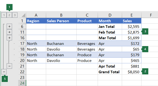
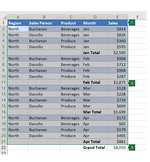
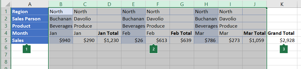
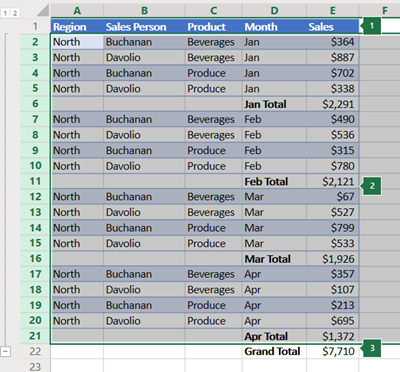
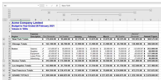
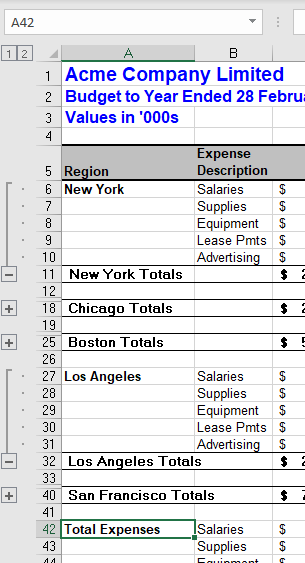
1. To display rows for a level, click the appropriate outline symbols.

2. Level 1 contains the total sales for all detail rows.

3. Level 2 contains total sales for each month in each region.

4. Level 3 contains detail rows — in this case, rows 17 through 20.

5. To expand or collapse data in your outline, click the plus and minus outline symbols, or press ALT+SHIFT+= to expand and ALT+SHIFT+- to collapse.

Make sure that each column of the data that you want to outline has a label in the first row (e.g., Region), contains similar facts in each column, and that the range you want to outline has no blank rows or columns.
If you want, your grouped detail rows can have a corresponding summary row—a subtotal. To create these, do one of the following:
- Insert summary rows by using the Subtotal command
  
  Use the Subtotal command, which inserts the SUBTOTAL function immediately below or above each group of detail rows and automatically creates the outline for you. For more information about using the Subtotal function, see SUBTOTAL function.
- Insert your own summary rows
  
  Insert your own summary rows, with formulas, immediately below or above each group of detail rows. For example, under (or above) the rows of sales data for March and April, use the SUM function to subtotal the sales for those months. The table later in this topic shows you an example of this.
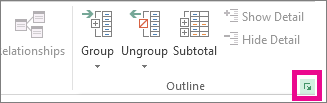
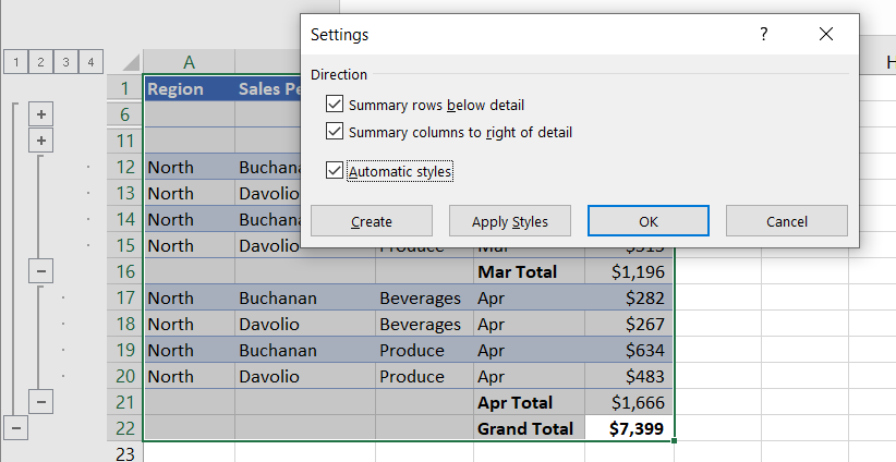
By default, Excel looks for summary rows below the details they summarize, but it’s possible to create them above the detail rows. If you created the summary rows below the details, skip to the next step (step 4). If you created your summary rows above your detail rows, on the Data tab, in the Outline group, click the dialog box launcher.

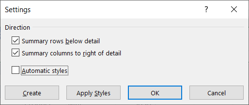
The Settings dialog box opens.

Then in the Settings dialog box, clear the Summary rows below detail checkbox, and then click OK.

Outline your data. Do one of the following:

Outline the data automatically

Select a cell in the range of cells you want to outline.
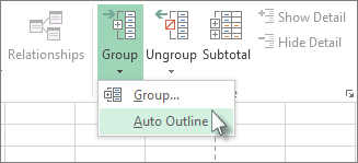
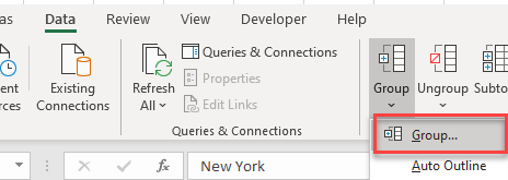
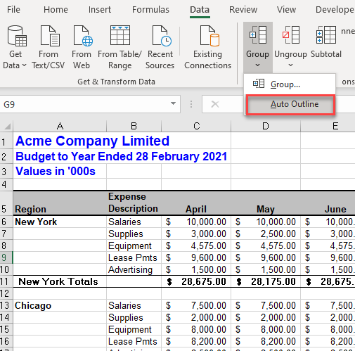
On the Data tab, in the Outline group, click the arrow under Group, and then click Auto Outline.

Outline the data manually

Important: When you manually group outline levels, it’s best to have all data displayed to avoid grouping the rows incorrectly.

To outline the outer group (level 1), select all of the rows the outer group will contain (i.e., the detail rows and if you added them, their summary rows).

1. The first row contains labels, and is not selected.

2. Since this is the outer group, select all the rows with subtotals and details.

3. Don’t select the grand total.

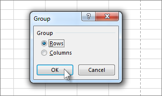
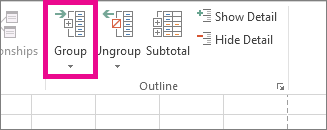
On the Data tab, in the Outline group, click Group. Then in the Group dialog box, click Rows, and then click OK.

Tip: If you select entire rows instead of just the cells, Excel automatically groups by row — the Group dialog box doesn’t even open.

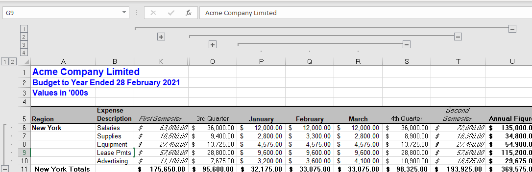
The outline symbols appear beside the group on the screen.

Optionally, outline an inner, nested group — the detail rows for a given section of your data.

Note: If you don’t need to create any inner groups, skip to step f, below.

For each inner, nested group, select the detail rows adjacent to the row that contains the summary row.

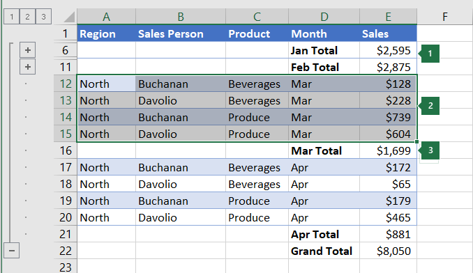
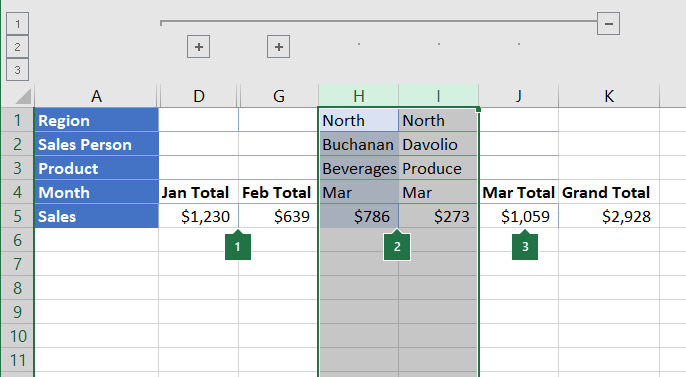
1. You can create multiple groups at each inner level. Here, two sections are already grouped at level 2.

2. This section is selected and ready to group.

3. Don’t select the summary row for the data you are grouping.

On the Data tab, in the Outline group, click Group.

Then in the Group dialog box, click Rows, and then click OK. The outline symbols appear beside the group on the screen.

Tip: If you select entire rows instead of just the cells, Excel automatically groups by row — the Group dialog box doesn’t even open.
Continue selecting and grouping inner rows until you have created all of the levels that you want in the outline.
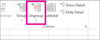
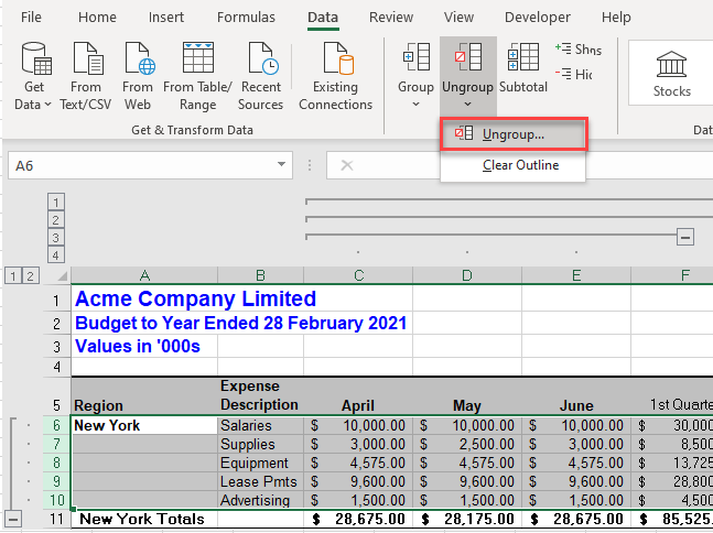
If you want to ungroup rows, select the rows, and then on the Data tab, in the Outline group, click Ungroup.

You can also ungroup sections of the outline without removing the entire level. Hold down SHIFT while you click the or for the group, and then on the Data tab, in the Outline group, click Ungroup.

Important: If you ungroup an outline while the detail data is hidden, the detail rows may remain hidden. To display the data, drag across the visible row numbers adjacent to the hidden rows. Then on the Home tab, in the Cells group, click Format, point to Hide & Unhide, and then click Unhide Rows.

Make sure that each row of the data that you want to outline has a label in the first column, contains similar facts in each row, and the range has no blank rows or columns.
Insert your own summary columns with formulas immediately to the right or left of each group of detail columns. The table listed in step 4 below shows you an example.

Note: To outline data by columns, you must have summary columns that contain formulas that reference cells in each of the detail columns for that group.
If your summary column is to the left of the detail columns, on the Data tab, in the Outline group, click the dialog box launcher.

The Settings dialog box opens.

Then in the Settings dialog box, clear the Summary columns to right of detail check box, and click OK.

To outline the data, do one of the following:

Outline the data automatically

Select a cell in the range.
On the Data tab, in the Outline group, click the arrow below Group and click Auto Outline.

Outline the data manually

Important: When you manually group outline levels, it’s best to have all data displayed to avoid grouping columns incorrectly.

To outline the outer group (level 1), select all of the subordinate summary columns, as well as their related detail data.

1. Column A contains labels.

2. Select all the detail and subtotal columns. Note that if you don’t select entire columns, when you click Group (on the Data tab in the Outline group) the Group dialog box will open and ask you to choose Rows or Columns.

3. Don’t select the grand total column.

On the Data tab, in the Outline group, click Group.

The outline symbol appears above the group.

To outline an inner, nested group of detail columns (level 2 or higher), select the detail columns adjacent to the column that contains the summary column.

1. You can create multiple groups at each inner level. Here, two sections are already grouped at level 2.

2. These columns are selected and ready to group. Note that if you don’t select entire columns, when you click Group (on the Data tab in the Outline group) the Group dialog box will open and ask you to choose Rows or Columns.

3. Don’t select the summary column for the data you are grouping.

On the Data tab, in the Outline group, click Group.

The outline symbols appear beside the group on the screen.

Continue selecting and grouping inner columns until you have created all of the levels that you want in the outline.
If you want to ungroup columns, select the columns, and then on the Data tab, in the Outline group, click Ungroup.

You can also ungroup sections of the outline without removing the entire level. Hold down SHIFT while you click the or for the group, and then on the Data tab, in the Outline group, click Ungroup.

If you ungroup an outline while the detail data is hidden, the detail columns may remain hidden. To display the data, drag across the visible column letters adjacent to the hidden columns. On the Home tab, in the Cells group, click Format, point to Hide & Unhide, and then click Unhide Columns

If you don’t see the outline symbols , , and , go to File > Options > Advanced, and then under the Display options for this worksheet section, select the Show outline symbols if an outline is applied check box, and then click OK.
Do one or more of the following:
- Show or hide the detail data for a group
  
  To display the detail data within a group, click the button for the group, or press ALT+SHIFT+=.
- To hide the detail data for a group, click the button for the group, or press ALT+SHIFT+-.
- Expand or collapse the entire outline to a particular level
  
  In the outline symbols, click the number of the level that you want. Detail data at lower levels is then hidden.
  
  For example, if an outline has four levels, you can hide the fourth level while displaying the rest of the levels by clicking .
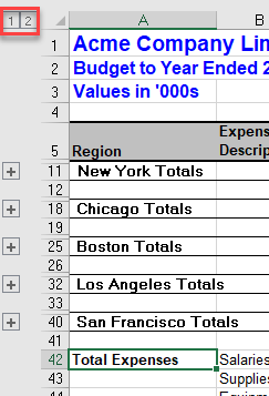
- Show or hide all of the outlined detail data
  
  To show all detail data, click the lowest level in the outline symbols. For example, if there are three levels, click .
- To hide all detail data, click .

For outlined rows, Microsoft Excel uses styles such as RowLevel_1 and RowLevel_2 . For outlined columns, Excel uses styles such as ColLevel_1 and ColLevel_2. These styles use bold, italic, and other text formats to differentiate the summary rows or columns in your data. By changing the way each of these styles is defined, you can apply different text and cell formats to customize the appearance of your outline. You can apply a style to an outline either when you create the outline or after you create it.

Do one or more of the following:

Automatically apply a style to new summary rows or columns

On the Data tab, in the Outline group, click the dialog box launcher.

The Settings dialog box opens.
Select the Automatic styles check box.

Apply a style to an existing summary row or column

Select the cells to which you want to apply a style.
On the Data tab, in the Outline group, click the dialog box launcher.

The Settings dialog box opens.
Select the Automatic styles check box, and then click Apply Styles.

You can also use autoformats to format outlined data.

If you don’t see the outline symbols , , and , go to File > Options > Advanced, and then under the Display options for this worksheet section, select the Show outline symbols if an outline is applied check box.
Use the outline symbols , , and to hide the detail data that you don’t want copied.

For more information, see the section, Show or hide outlined data.
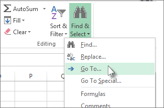
Select the range of summary rows.
On the Home tab, in the Editing group, click Find & Select, and then click Go To.
Click Go To Special.
Click Visible cells only.
Click OK, and then copy the data.

Note: No data is deleted when you hide or remove an outline.

Hide an outline

Go to File > Options > Advanced, and then under the Display options for this worksheet section, uncheck the Show outline symbols if an outline is applied check box.

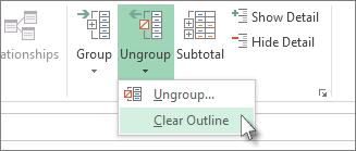
Remove an outline

Click the worksheet.
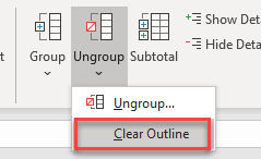
One the Data tab, in the Outline group, click Ungroup and click Clear Outline.

Important: If you remove an outline while the detail data is hidden, the detail rows or columns may remain hidden. To display the data, drag across the visible row numbers or column letters adjacent to the hidden rows and columns. On the Home tab, in the Cells group, click Format, point to Hide & Unhide, and then click Unhide Rows or Unhide Columns.

Imagine that you want to create a summary report of your data that only displays totals accompanied by a chart of those totals. In general, you can do the following:

Create a summary report
1. Outline your data.
  
  For more information, see the sections Create an outline of rows or Create an outline of columns.
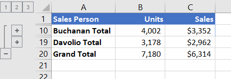
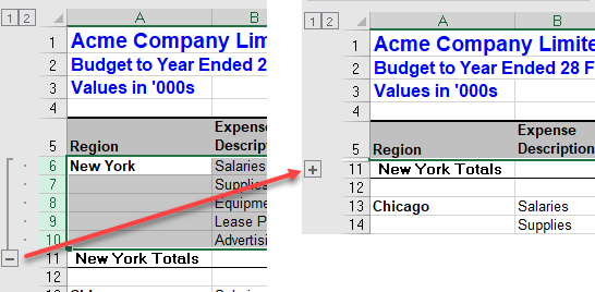
2. Hide the detail by clicking the outline symbols , , and to show only the totals as shown in the following example of a row outline:
3. For more information, see the section, Show or hide outlined data.
Chart the summary report
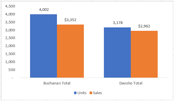
1. Select the summary data that you want to chart.
  
  For example, to chart only the Buchanan and Davolio totals, but not the grand totals, select cells A1 through C19 as shown in the above example.
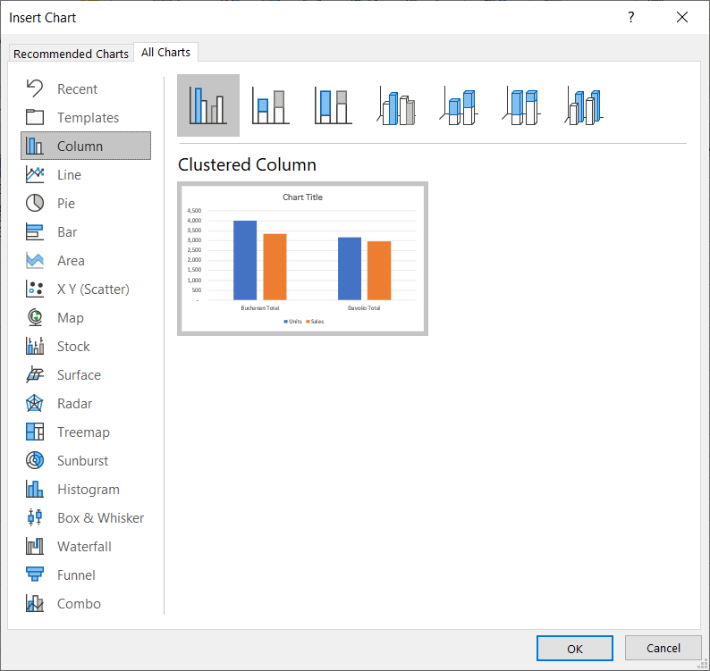
2. Click Insert > Charts > Recommended Charts, then click the All Charts tab and choose your chart type.
  
  For example, if you chose the Clustered Column option, your chart would look like this:
  
  If you show or hide details in the outlined list of data, the chart is also updated to show or hide the data.

You can group (or outline) rows and columns in Excel for the web.

Note: Although you can add summary rows or columns to your data (by using functions such as SUM or SUBTOTAL), you cannot apply styles or set a position for summary rows and columns in Excel for the web.

Create an outline of rows or columns

Outline of rows in Excel Online

The first column contains labels.
The detail rows and summary rows are grouped in the outline.
The grand total is not grouped in the outline.

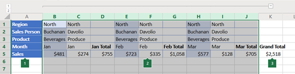
Outline of columns in Excel Online

The first row contains labels.
The detail columns and summary columns are grouped in the outline.
The grand total is not grouped in the outline.

Make sure that each column (or row) of the data that you want to outline has a label in the first row (or column), contains similar facts in each column (or row), and that the range has no blank rows or columns.
Select the data (including any summary rows or columns).
On the Data tab, in the Outline group, click Group > Group Rows or Group Columns.
Optionally, if you want to outline an inner, nested group — select the rows or columns within the outlined data range, and repeat step 3.
Continue selecting and grouping inner rows or columns until you have created all of the levels that you want in the outline.

Ungroup rows or columns

To ungroup, select the rows or columns, and then on the Data tab, in the Outline group, click Ungroup and select Ungroup Rows or Ungroup Columns.

Show or hide outlined data

Do one or more of the following:

Show or hide the detail data for a group

To display the detail data within a group, click the for the group, or press ALT+SHIFT+=.
To hide the detail data for a group, click the for the group, or press ALT+SHIFT+-.

Expand or collapse the entire outline to a particular level

In the outline symbols, click the number of the level that you want. Detail data at lower levels is then hidden.
For example, if an outline has four levels, you can hide the fourth level while displaying the rest of the levels by clicking .

Show or hide all of the outlined detail data

To show all detail data, click the lowest level in the outline symbols. For example, if there are three levels, click .
To hide all detail data, click .

Need more help?

You can always ask an expert in the Excel Tech Community or get support in the Answers community.

Guide on How to Group in Excel

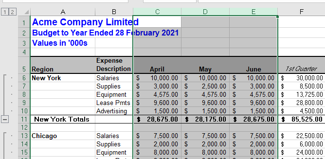
Grouping rows and columns in Excel[1] is critical for building and maintaining a well-organized and well-structured financial model. Using the Excel group function is the best practice when it comes to staying organized, as you should never hide cells in Excel. This guide will show you how to group in Excel with step-by-step instructions, examples, and screenshots.

Keyboard Shortcuts Sheet

Looking to be an Excel wizard? Increase your productivity with CFI’s comprehensive keyboard shortcuts guide.

Excel Group Function

The Excel group function is one of the best secrets a world-class financial analyst uses to make their work extremely organized and easy for other users of the spreadsheet to understand.

Reasons to use the Excel Group Function:

To easily expand and contract sections of a worksheet
To minimize schedules or side calculations that other users might not need
To keep information organized
As a substitute for creating new sheets (tabs)
As a superior alternative to hiding cells

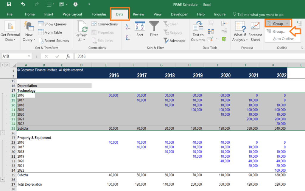
The function is found in the Data section of the Ribbon, then Group.

Example of How to Group in Excel

Let’s look at a simple exercise to see how it works. Suppose we have a schedule in a worksheet that is becoming quite long, and we want to reduce the amount of detail that’s shown. The screenshots below will show you how to properly implement grouping in Excel.

Here are the steps to follow to group rows:

Select the rows you wish to add grouping to (entire rows, not just individual cells)
Go to the Data Ribbon
Select Group
Select Group again

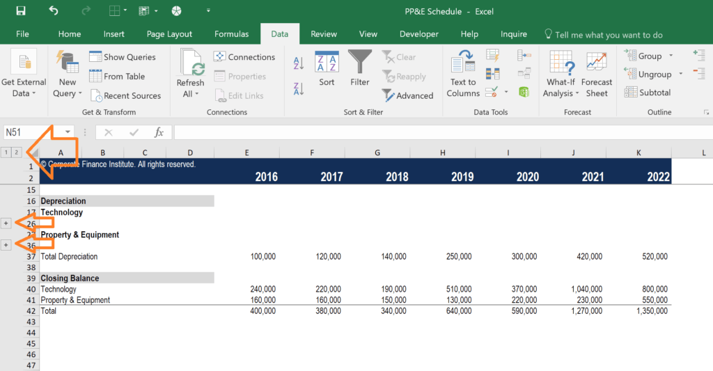
You can repeat the steps above as many times as you like, and you can also apply it to columns as well.

Once you’re finished, you can press the “-” buttons in the margin to collapse the rows or columns.

If you want to expand them again, press the “+” buttons in the margin, as shown in the screenshot below.

There is also a “1” button in the top left corner to collapse all groups, and a “2” button to expand all groups.

Why You Should Never Hide Cells in Excel

Though many people do it, you should never hide cells in Excel (or spreadsheets either, for that matter). The reason is that Excel does not make it clear to the user of the spreadsheet that cells have been hidden, and thus they may go unnoticed.

The only way to see that cells are hidden is to notice that the row number or column number suddenly jumps (e.g., from row 25 to row 167).

Since other users of the spreadsheet may not notice this (and you may forget yourself) you should never hide cells in Excel.

Download Excel Group Template

You can download the Template for free if you wish to use it as an example or starting point for how to group in Excel and apply it to your own work and financial analysis.

Additional Resources

Thank you for reading CFI’s guide to Group in Excel. To continue learning and advancing your career, these additional CFI resources will be helpful:

List of 300+ Excel Functions
Keyboard Shortcuts
What is Financial Modeling?
Financial Modeling Courses
See all Excel resources

Источник

Microsoft Excel lets you sort data using one or more cells in a spreadsheet. Grouping cells in Excel gives you a chance to have visuals to clear data. Not only this, but you can even make some changes in the outline as per your needs. When you need to make a truly defined data sheet, grouping comes in.

With Excel, it will be easier to group data into multiple categories so that you can read data conveniently. Here in this post, you will get to know some useful methods that help in grouping cells in Excel. Let’s dive in:

Sometimes when your spreadsheet is full of information, it could be challenging to organize data for better understanding. With a list of data, you can easily manage to wrap it up.

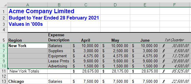
Below you will find a dataset containing product B, the name of some product brands in column C, and sales in January, February, and March in columns D, E, and F. In column G, you can see the net sale of all products. Suppose that the individual sales in individual months are unwanted information for us and we don’t want to have the sales for separate brands as well.

So, how would it happen? Do you have any idea? We’ll group the data separately that we don’t need.

Grouping Cells in Excel Using Group Feature

Using the group feature, you can hide some cells and icons from your sheet so that they are not visible to you. The group feature lets you group cells by following the steps given below:

First of all, select the data that needed to be grouped. Here we’ll select the data cells from columns D, E, and F.
From the ribbon, click on the Data tab and then choose the Group drop-down menu.
Now, in the outline toolbar click on the option Group.

Right after this step, you will see a minus sign added to the outline above the selected cells. Using this sign, we will group the cells.
Considering the above data, now suppose we need to group the cells from rows 5, 6, 7, and 8. Select cells from these rows.
Moreover, open the Data tab from the Excel toolbar and choose the Group option.

Here we go. Whenever you need to hide cells you can easily manage to do this because these cells are grouped now.

Apply Subtotal Command to Group Cells

Using the Excel subtotal feature helps in the data analysis. It also helps in making groups and then further uses them for sum, average, and other functions on the grouped cells. Below we have some easy-to-follow steps:

Select the entire sheet by clicking on the green triangle given at the top of the left side.
Now, open the Data tab from the ribbon.
Later on, choose the Subtotal option given under the Outline section.

You will see an Excel pop-up window appears. Click on the OK button.
Now, you can see the Subtotal dialog box and then choose the columns you need to group.
Click OK.

Following this step will make new rows after each product and that will be the net sale for each month.
The cells on the left side of your sheet are now grouped.

Keyboard Shortcuts to Group Cells in Excel

Most of the time, people don’t want to be a part of lengthy steps that’s why they prefer trying keyboard shortcuts that are helpful in every way. It also helps in increasing the level of productivity. For grouping cells in Excel, we can use keyboard shortcuts. For this, follow the steps:

First, choose the cells that needed to be grouped. Here we will select columns D, E, and F.
Press the Shift + Alt + Right Arrow keys from the keyboard.
That’s it. Your cells are now grouped.

Summing Up

Now, you are fully aware of the methods that help in grouping cells in Excel. Try any of the above-mentioned methods because each method has its own significance. Also, share these methods with others so that you can be a part of spreading the knowledge thread.

Источник

При обработке большого объема данных довольно часто требуется их упорядочивание. Специально для этого в программе Excel предусмотрены различные функции, одной из которых является группировка. С ее помощью, как следует из названия, можно сгруппировать данные, а также, скрыть неактуальную информацию. Давайте разберемся, как это работает.

Настраиваем параметры функции
Группируем данные по строкам
Группируем столбцы
Создаем многоуровневую группировку
Разгруппировываем данные
Заключение

Настраиваем параметры функции

Чтобы в конечном счете получить желаемый результат, для начала следует выполнить настройки самой функции. Для этого выполняем следующие шаги:

Переключившись во вкладку “Данные” щелкаем по кнопке “Структура” и в открывшемся перечне команд – по небольшому значку в виде стрелки, направленной по диагонали вниз.
На экране отобразится небольшое окошко с параметрами функции. Здесь мы можем настроить отображение итогов. Ставим галочки напротив нужных опций (в т.ч. автоматические стили) и жмем кнопку OK.Примечание: расположение итоговых данных в строках под данными многим кажется неудобным, поэтому данный параметр можно выключить.
Все готово, теперь можем перейти, непосредственно, к самой группировке данных.

Группируем данные по строкам

Для начала давайте рассмотрим, как можно сгруппировать строки:

Вставляем новую строку над или под строками, которые хотим сгруппировать (зависит от того, какой вид расположения итогов по строкам мы выбрали). Как это сделать, читайте в нашей статье – “Как добавить новую строку в Excel“.
В самой левой ячейке добавленной строки пишем название, которое хотим присвоить группе.
Любым удобным способом, например, с помощью зажатой левой кнопки мыши производим выделение ячеек строк (кроме итоговой), которые требуется сгруппировать. Во вкладке “Данные” щелкаем по кнопке “Структура” и в открывшемся списке выбираем функцию “Группировать”. Щелкнуть нужно именно по значку команды, а не по ее названию. Если же нажать на последнее (со стрелкой вниз), откроется еще одно подменю, в котором следует нажать на одноименную кнопку.
В появившемся окошке отмечаем пункт “строки” (должен быть выбран по умолчанию) и подтверждаем действие нажатием OK.Примечание: Если вместо ячеек выделить все строки целиком на вертикальной панели координат, а затем применить группировку, то промежуточного окна с выбором строки или столбца не будет, так как программа сразу понимает, что именно ей необходимо сделать.
Группа создана, о чем свидетельствуют появившаяся на панели координат полоска со знаком “минус”. Это означает, что сгруппированные данные раскрыты. Чтобы их скрыть, нажимам по минусу или кнопке с цифрой “1” (самый верхний уровень группировки).
Теперь строки скрыты. Чтобы их обратно раскрыть, нажимаем по значку “плюса”, который появился вместо “минуса” (или по кнопке “2”).

Группируем столбцы

Чтобы сгруппировать столбцы, придерживаемся примерно такого же алгоритма действий, описанного выше:

Вставляем столбец справа или слева от группируемых – зависит от выбранного параметра в настройках функции. Подробнее о том, как это сделать, читайте в нашей статье – “Как вставить столбец в таблицу Эксель“.
Пишем название в самой верхней ячейке нового столбца.
Выделяем ячейки группируемых столбцов (за исключением добавленного) и применяем функцию группировки.
Ставим отметку напротив варианта “столбцы” и кликам OK.Примечание: как и в случае с группировкой строк, при выделении столбцов целиком на горизонтальной панели координат, группировка данных будет выполнена сразу, минуя промежуточное окно с выбором элементов.
Задача успешно выполнена.

Создаем многоуровневую группировку

Возможности программы позволяют выполнять как одноуровневые, так и многоуровневые группировки. Вот как это делается:

В раскрытом состоянии главной группы, внутри которой планируется создать еще одну, выполняем действия, рассмотренные в разделах выше в зависимости от того, с чем мы работаем – со строками или столбцами.
Таким образом, мы получили многоуровневую группировку.

Разгруппировываем данные

Когда ранее выполненная группировка столбцов или строк больше не нужна или требуется выполнить ее иначе, можно воспользоваться обратной функцией – “Разгруппировать”:

Производим выделение сгруппированных элементов, после чего все в той же вкладке “Данные” в группе инструментов “Структура” выбираем команду “Разгруппировать”. Жмем именно по значку, а не по названию.
В открывшемся окне ставим отметку напротив требуемого пункта (в нашем случае – “строки”) и нажимаем OK.Примечание: в случае многоуровневой группировки или наличия нескольких групп данных, каждую из них необходимо расформировать отдельно.
Вот и все, что требовалось сделать.

Заключение

Группировка данных выполняется в несколько кликов и не требует особых навыков в работе с программой, однако, данный прием позволяет существенно сэкономить время, когда приходится иметь дело с большим объемом информации. Это делает функцию одной из самых полезных и незаменимых в Excel.

Источник

This tutorial will demonstrate how to Group Cells (Rows / Columns) in Excel & Google Sheets.

Grouping or outlining data in Excel allows us to hide or show rows or columns depending on how much detail we wish to see on the screen. Different levels can be displayed according to your needs. Excel allows up to 8 levels of grouping. To use the group function in Excel, the data really needs to be organized in your worksheet in a specific way that works with the grouping functionality.

Manually Grouping or Ungrouping Rows

1. To group a number of rows together, first, highlight the rows you wish to group.

2. In the Ribbon, select Data > Outline > Group >Group.

3. A small minus sign will be added into the outline bar on the left of the screen. Clicking on the minus sign allows us to collapse the group and the minus sign will then change to a plus sign indicating that there is hidden data within the outline.

4. We can repeat manual grouping to add more groups to the worksheet as required.

5. As well as using the plus and minus outline symbols, we can also use the 1 or 2 in the top left hand corner of the screen to expand or collapse all the groups.

6. Clicking on the 1 will collapse all the groups while clicking on 2 will expand all the groups.

Manually Grouping or Ungrouping Columns

1. To group a number of columns together, first, highlight the columns you wish to group. This can be done if you have rows already grouped or not.

2. In the Ribbon, select Data > Outline > Group >Group to group the columns together. Repeat this until you have created all the groups that you require.

3. Once we have grouped our rows and / or columns, we can add a new level but grouping once again. This will add a third level of grouping to the outline symbols in the top left hand corner of the screen.

4. Once again, we can repeat this across our worksheet, and add up to 8 levels of grouping.

Ungrouping Rows or Columns

1. Highlight the group you wish to ungroup and then, in the Ribbon, select Data > Outline > Ungroup > Ungroup.

This will only remove the one group.

2. To remove all the grouping in the worksheet, click anywhere in the data and then, in the Ribbon, select Data > Outline > Ungroup > Clear Outline.

Auto-Outline

We can use the Auto Outline function of Excel as long as our data is logically organized so that Excel recognizes the groups within the rows and columns. There must not be any blank rows in the data and the data must be summed or subtotaled at each level.

1. Click anywhere in the data where you wish the outline to be created and then, in the Ribbon, select Data > Outline > Group > Auto Outline.

2. Excel will create as many grouping levels as the logical layout of the data allows.

How to Group Cells in Google Sheets

Google Sheets only allows us to manually group or ungroups rows and columns of data.

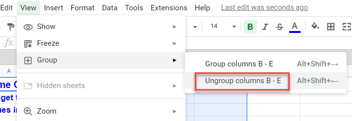
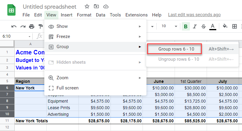
1. Select the rows you wish to group and then, in the Menu, select View > Group > Group rows (the number of rows selected will be shown).

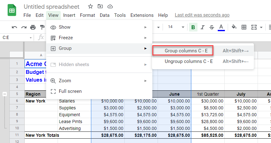
2. Similarly, select the columns you wish to group and then in the Menu, select View > Group > Group columns (the number of columns selected will be shown).

3. To ungroup rows or columns, click in the group you wish to ungroup and then in the Menu, select View > Group > Ungroup (rows or columns).

Источник

Create an outline of rows or columns

Ungroup rows or columns

Show or hide outlined data

Need more help?

See Also

Guide on How to Group in Excel

Keyboard Shortcuts Sheet

Excel Group Function

Example of How to Group in Excel

Why You Should Never Hide Cells in Excel

Download Excel Group Template

Additional Resources

Grouping Cells in Excel Using Group Feature

Apply Subtotal Command to Group Cells

Keyboard Shortcuts to Group Cells in Excel

Summing Up

Настраиваем параметры функции

Группируем данные по строкам

Группируем столбцы

Создаем многоуровневую группировку

Разгруппировываем данные

Заключение

Manually Grouping or Ungrouping Rows

Manually Grouping or Ungrouping Columns

Ungrouping Rows or Columns

Auto-Outline

How to Group Cells in Google Sheets