
Содержание
- Group rows of data (Power Query)
- Group in Excel
- Guide on How to Group in Excel
- Keyboard Shortcuts Sheet
- Excel Group Function
- Example of How to Group in Excel
- Why You Should Never Hide Cells in Excel
- Download Excel Group Template
- Additional Resources
- Group Columns in Excel
- Excel Column Grouping
- How to Use Column Grouping in Excel? (with Examples)
- Example #1
- Example #2
- How to Hide or Unhide the Group Column?
- Shortcut Keys to Hide or Unhide Column Grouping in Excel
- Why you should use the Excel Column Grouping
- Why you should not use the Excel Column Grouping
- Things to Remember
- Recommended Articles
- How to group rows in Excel to collapse and expand them
- Grouping rows in Excel
- How to group rows automatically (create an outline)
- How to group rows manually
- 1. Create outer groups (level 1)
- 2. Create nested groups (level 2)
- 3. Add more grouping levels if necessary
- How to collapse rows in Excel
- Collapse rows within a group
- Collapse or expand the entire outline to a specific level
- How to expand rows in Excel
- How to remove outline in Excel
- How to remove the entire outline
- How to ungroup a certain group of rows
- Excel grouping tips
- How to calculate group subtotals automatically
- Apply default Excel styles to summary rows
- How to select and copy only visible rows
- How to hide and show outline symbols
- The outline symbols don’t show up in Excel
Group rows of data (Power Query)
In Power Query, you can group the same values in one or more columns into a single grouped row. You can group a column by using an aggregate function or group by a row.
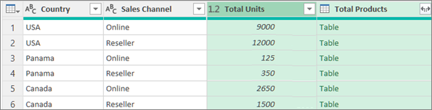
The following procedures are based on this query data example:
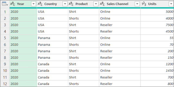
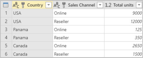
You can group data by using an aggregate function, such as Sum and Average. For example, you want to summarize the total units sold at the country and sales channel level, grouped by the Country and Sales Channel columns.
To open a query, locate one previously loaded from the Power Query Editor, select a cell in the data, and then select Query > Edit. For more information see Create, edit, and load a query in Excel.
Select Home > Group by.
In the Group by dialog box, select Advanced to select more than one column to group by.
To add another column, select Add Grouping.
Tip To delete or move a grouping, select More (…) next to the grouping name box.
Select the Country and Sales Channel columns.
In the next section:
New column name Enter «Total units» for the new column header.
Operation Select Sum. The aggregations available are Sum, Average, Median, Min, Max, Count Rows, and Count Distinct Rows.
Column Select Units to specify which column to aggregate.
A Row Operation does not require a column, because data is grouped by a row in the Group By dialog box. There are two choices when you create a new column:
Count Rows which displays the number of rows in each grouped row.
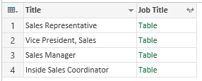
All Rows An inner Table value is inserted. It contains all the rows for the columns you grouped by. You can later expand the columns if you want. For more information, see Work with a List, Record, or Table structured column.
For example, to group by all rows, you want the total units sold and you want two other columns that give you the name and units sold for the top-performing product, summarized at the country and sales channel level.
To open a query, locate one previously loaded from the Power Query Editor, select a cell in the data, and then select Query > Edit. For more information see Create, load, or edit a query in Excel.
Select Home > Group by.
In the Group by dialog box, select Advanced to select more than one column to group by.
Add a column to aggregate by selecting Add aggregation at the bottom of the dialog box.
Tip To delete or move an aggregation, select More (…) next to the column box.
Under Group by, select the Country and Sales Channel columns.
Create two new columns by doing the following:
Aggregation Aggregate the Units column by using the Sum operation. Name this column Total units.
All rows Add a new Products column by using the All rows operation. Name this column Total products. Because this operation acts upon all rows, you don’t need to make a selection under Column and so it is not available.
Источник
Group in Excel
The best way to keep spreadsheets organized
Guide on How to Group in Excel
Grouping rows and columns in Excel[1] is critical for building and maintaining a well-organized and well-structured financial model. Using the Excel group function is the best practice when it comes to staying organized, as you should never hide cells in Excel. This guide will show you how to group in Excel with step-by-step instructions, examples, and screenshots.

Keyboard Shortcuts Sheet
Looking to be an Excel wizard? Increase your productivity with CFI’s comprehensive keyboard shortcuts guide.
Excel Group Function
The Excel group function is one of the best secrets a world-class financial analyst uses to make their work extremely organized and easy for other users of the spreadsheet to understand.
Reasons to use the Excel Group Function:
- To easily expand and contract sections of a worksheet
- To minimize schedules or side calculations that other users might not need
- To keep information organized
- As a substitute for creating new sheets (tabs)
- As a superior alternative to hiding cells
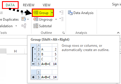
The function is found in the Data section of the Ribbon, then Group.
Example of How to Group in Excel
Let’s look at a simple exercise to see how it works. Suppose we have a schedule in a worksheet that is becoming quite long, and we want to reduce the amount of detail that’s shown. The screenshots below will show you how to properly implement grouping in Excel.
Here are the steps to follow to group rows:
- Select the rows you wish to add grouping to (entire rows, not just individual cells)
- Go to the Data Ribbon
- Select Group
- Select Group again
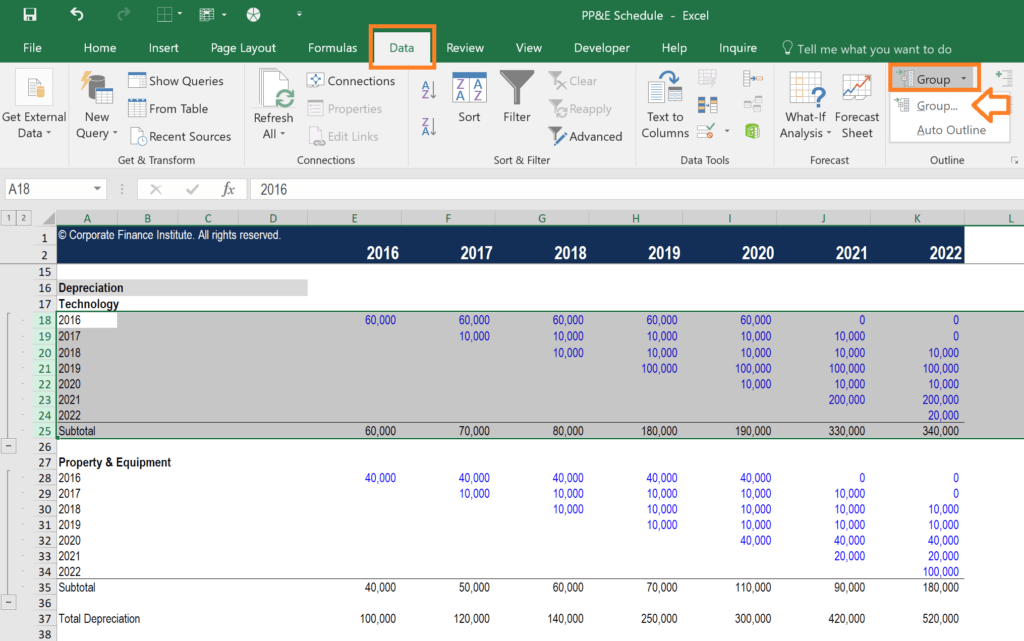
You can repeat the steps above as many times as you like, and you can also apply it to columns as well.
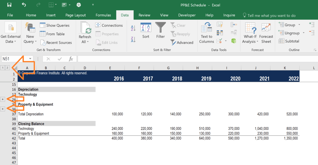
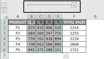
Once you’re finished, you can press the “-” buttons in the margin to collapse the rows or columns.
If you want to expand them again, press the “+” buttons in the margin, as shown in the screenshot below.
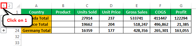
There is also a “1” button in the top left corner to collapse all groups, and a “2” button to expand all groups.
Why You Should Never Hide Cells in Excel
Though many people do it, you should never hide cells in Excel (or spreadsheets either, for that matter). The reason is that Excel does not make it clear to the user of the spreadsheet that cells have been hidden, and thus they may go unnoticed.
The only way to see that cells are hidden is to notice that the row number or column number suddenly jumps (e.g., from row 25 to row 167).
Since other users of the spreadsheet may not notice this (and you may forget yourself) you should never hide cells in Excel.
Download Excel Group Template
You can download the Template for free if you wish to use it as an example or starting point for how to group in Excel and apply it to your own work and financial analysis.
Additional Resources
Thank you for reading CFI’s guide to Group in Excel. To continue learning and advancing your career, these additional CFI resources will be helpful:
Источник
Group Columns in Excel


Excel Column Grouping
Group Column in Excel means bringing one or more columns together in an Excel worksheet. It enables an option to contract or expand the column, and Excel provides us a button to do so. To group columns, we must select two or more columns, and then from the “Data” tab in the “Outline” section, we have the option to group the columns.
Table of contents
How to Use Column Grouping in Excel? (with Examples)
Example #1
Following are the steps of Excel column grouping:
- We must select the data first that we are using to group the column in Excel.

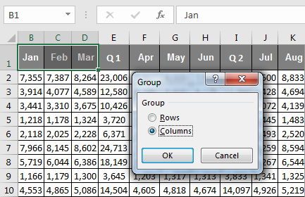
Then, go to the “Data” option in the Excel toolbar and select the “Group” option in the “Outline” toolbar, as shown in the below screenshot.

When we click on the “Group,” it will enable us to group the particular column in the Excel spreadsheet. As shown below in the screenshot, the minus sign symbol is added to the outline above the selected columns.

When we hide columns C and D in a spreadsheet, it is the result. It automatically enables the grouping option in the spreadsheet.
Example #2
- Step 1: We must first select columns B and C.
- Step 2: Go to the “Data” option in the excel toolbarExcel ToolbarThe toolbar, also known as the quick access toolbar, is located on the left top-most side of the excel window and has only a few options by default, such as save, redo, and undo. Users can, however, customize it to their liking and add any option or button to make it easier to access the commands.read more and select the “Group” option in the outline toolbar, as shown below.

- Step 3: Next, go to the option group and make the group of a column selected.

Now, we can see the two minus signs; two groups are created in a particular spreadsheet that we want to group.
How to Hide or Unhide the Group Column?
- Step 1: First, We must click on the created minus sign while grouping the column.

- Step 2: When we click on the minus sign, a column will collapse, resulting in the hide in a column.

- Step 3: Once we click on the minus sign, it automatically shows the plus sign, which means that if we want to unhide the column, click on the plus sign to unhide the columns.
- Step 4: We can likewise utilize the small numbers in the upper left corner. They let us cover up and unhide all groupings of a similar dimension without a moment’s delay. For instance, in the table on the screen capture, clicking on 2 will conceal columns B and D. This is particularly helpful if we made a progressive collection system. Likewise, clicking on 3 will unhide or hide columns C and D.

Shortcut Keys to Hide or Unhide Column Grouping in Excel
- Step 1: First, we must select the data. Then, press the Shortcut Excel KeysShortcut Excel KeysAn Excel shortcut is a technique of performing a manual task in a quicker way.read more – Shift + Alt + right arrow. We may see the dialog box in the Excel spreadsheet as follows:


- Step 2: Select the radio button on a column to hide the columns in excelHide The Columns In ExcelThe methods to hide columns in excel are — hide columns using right-click option, hide columns using shortcut cut key, hide columns using column width, hide columns using VBA code.read more .

- Step 3: Click on the “OK.” Now, we can hide and unhide the columns in excelUnhide The Columns In ExcelUsing the Home tab of the Excel ribbon, using the shortcut key, using the context menu, altering the column width, using the ctrl+G (go to) command, and using the ctrl+F (find) command are some of the ways to unhide a column in Excel.read more .

Why you should use the Excel Column Grouping
- To effectively expand and contract the section or areas of a worksheet.
- To limit schedules or side estimations that different users probably would not require while working in Excel worksheets.
- To keep data composed and in an organized structure.
- To make new sheets (tabs) as a substitute.
- It is a better option than hiding cells.
- It is a better function as compared to hiding the column function.
- It helps to set up the grouping level.
Why you should not use the Excel Column Grouping
- We would not be able to make a group of cells that are not adjacent.
- If we manage different worksheets and need to assemble similar lines/columns on numerous worksheets in the meantime, it is impossible to use this function.
- We always need to check that the data is in a sorted form.
- We always need to check while grouping the column in Excel to select the correct column that needs to group.
Things to Remember
- We would not be able to add the calculated items to grouped fields in the Excel spreadsheet.
- It is impractical to choose a few non-nearby columns.
- Clicking on the minus icon may hide the column, and the icon may change to the plus sign letting us instantly unhide the data.
- We can select the range and press “Shift + Alt + left arrow” to remove the grouping from the Excel spreadsheet.
Recommended Articles
This article is a guide to Group Columns in Excel. We discuss using group Excel columns, examples, and downloadable Excel templates here. You may also look at these useful functions in Excel: –
Источник
How to group rows in Excel to collapse and expand them
 by Svetlana Cheusheva, updated on March 17, 2023
The tutorial shows how to group rows in Excel to make complicated spreadsheets easier to read. See how you can quickly hide rows within a certain group or collapse the entire outline to a particular level.
Worksheets with a lot of complex and detailed information are difficult to read and analyze. Luckily, Microsoft Excel provides an easy way to organize data in groups allowing you to collapse and expand rows with similar content to create more compact and understandable views.
Grouping rows in Excel
Grouping in Excel works best for structured worksheets that have column headings, no blank rows or columns, and a summary row (subtotal) for each subset of rows. With the data properly organized, use one of the following ways to group it.
How to group rows automatically (create an outline)
If your dataset contains just one level of information, the fastest way would be to let Excel group rows for you automatically. Here’s how:
- Select any cell in one of the rows you want to group.
- Go to the Data tab >Outline group, click the arrow under Group, and select Auto Outline.
That’s all there is to it!
Here is an example of what kind of rows Excel can group: 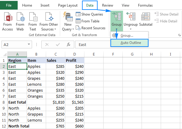
As shown in the screenshot below, the rows have been grouped perfectly and the outline bars representing different levels of data organization have been added to the left of column A. 
Note. If your summary rows are located above a group of detail rows, before creating an outline, go to the Data tab > Outline group, click the Outline dialog box launcher, and clear the Summary rows below detail checkbox.
Once the outline is created, you can quickly hide or show details within a certain group by clicking the minus  or plus
  sign for that group. You can also collapse or expand all rows to a particular level by clicking on the level buttons
  in the top-left corner of the worksheet. For more information, please see How to collapse rows in Excel.
How to group rows manually
If your worksheet contains two or more levels of information, Excel’s Auto Outline may not group your data correctly. In such a case, you can group rows manually by performing the steps below.
Note. When creating an outline manually, make sure your dataset does not contain any hidden rows, otherwise your data may be grouped incorrectly.
1. Create outer groups (level 1)
Select one of the larger subsets of data, including all of the intermediate summary rows and their detail rows.
In the dataset below, to group all data for row 9 (East Total), we select rows 2 through 8. 
On the Data tab, in the Outline group, click the Group button, select Rows, and click OK. 
This will add a bar on the left side of the worksheet that spans the selected rows: 
In a similar manner, you create as many outer groups as necessary.
In this example, we need one more outer group for the North region. For this, we select rows 10 to 16, and click Data tab > Group button > Rows.
That set of rows is now grouped too: 
Tip. To create a new group faster, press the Shift + Alt + Right Arrow shortcut instead of clicking the Group button on the ribbon.
2. Create nested groups (level 2)
To create a nested (or inner) group, select all detail rows above the related summary row, and click the Group button.
For example, to create the Apples group within the East region, select rows 2 and 3, and hit Group. To make the Oranges group, select rows 5 through 7, and press the Group button again.
Similarly, we create nested groups for the North regions, and get the following result: 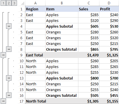
3. Add more grouping levels if necessary
In practice, datasets are seldom complete. If at some point more data is added to your worksheet, you will probably want to create more outline levels.
As an example, let’s insert the Grand total row in our table, and then add the outermost outline level. To have it done, select all the rows except for the Grand Total row (rows 2 through 17), and click Data tab > Group button > Rows.
As shown in the screenshot below, our data is now grouped in 4 levels:
- Level 1: Grand total
- Level 2: Region totals
- Level 3: Item subtotals
- Level 4: Detail rows

Now that we have an outline of rows, let’s see how it makes our data easier to view.
How to collapse rows in Excel
One of the most useful features of Excel grouping is the ability to hide and show the detail rows for a particular group as well as to collapse or expand the entire outline to a certain level in a mouse click.
Collapse rows within a group
To collapse the rows in a particular group, just click the minus button at the bottom of that group’s bar.
For example, this is how you can quickly hide all detail rows for the East region, including subtotals, and show only the East Total row: 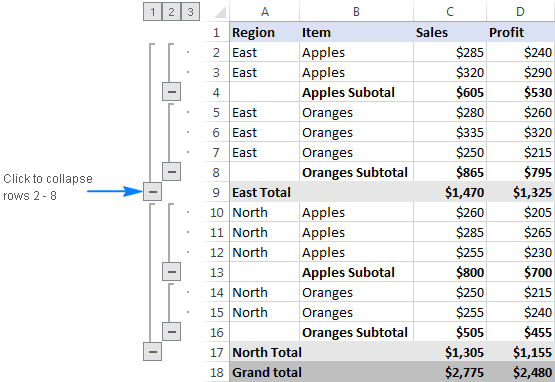
Another way to collapse rows in Excel is to select any cell in the group and click the Hide Detail button on the Data tab, in the Outline group: 
Either way, the group will be minimized to the summary row, and all of the detail rows will be hidden.
Collapse or expand the entire outline to a specific level
To minimize or expand all the groups at a particular level, click the corresponding outline number at the top left corner of your worksheet.
Level 1 displays the least amount of data while the highest number expands all the rows. For example, if your outline has 3 levels, you click number 2 to hide the 3rd level (detail rows) while displaying the other two levels (summary rows).
In our sample dataset, we have 4 outline levels, which work this way:
- Level 1 shows only Grand total (row 18 ) and hides all other rows.
- Level 2 displays Grand total and Region subtotals (rows 9, 17 and 18).
- Level 3 displays Grand total, Region and Item subtotals (rows 4, 8, 9, 18, 13, 16, 17 and 18).
- Level 4 shows all the rows.
The following screenshot demonstrates the outline collapsed to level 3. 
How to expand rows in Excel
To expand the rows within a certain group, click any cell in the visible summary row, and then click the Show Detail button on the Data tab, in the Outline group: 
Or click the plus sign for the collapsed group of rows that you want to expand: 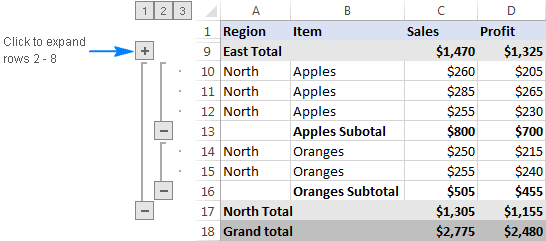
How to remove outline in Excel
In case you want to remove all row groups at once, then clear the outline. If you want to remove just some of the row groups (e.g. nested groups), then ungroup the selected rows.
How to remove the entire outline
Go to the Data tab > Outline group, click the arrow under Ungroup, and then click Clear Outline. ![]()
- Removing outline in Excel does not delete any data.
- If you remove an outline with some collapsed rows, those rows might remain hidden after the outline is cleared. To display the rows, use any of the methods described in How to unhide rows in Excel.
- Once the outline is removed, you won’t be able to get it back by clicking the Undo button or pressing the Undo shortcut ( Ctrl + Z ). You will have to recreate the outline from scratch.
How to ungroup a certain group of rows
To remove grouping for certain rows without deleting the whole outline, do the following:
- Select the rows you want to ungroup.
- Go to the Data tab >Outline group, and click the Ungroup button. Or press Shift + Alt + Left Arrow which is the Ungroup shortcut in Excel.
- In the Ungroup dialog box, select Rows and click OK.
For example, here’s how you can ungroup two nested row groups (Apples Subtotal and Oranges Subtotal) while keeping the outer East Total group: 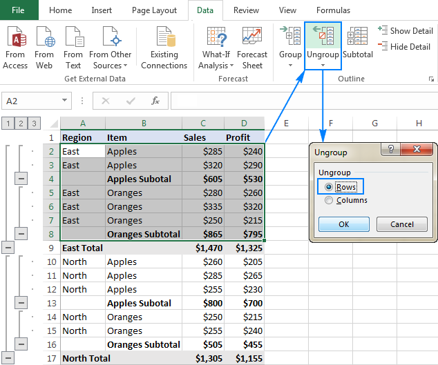
Note. It is not possible to ungroup non-adjacent groups of rows at a time. You will have to repeat the above steps for each group individually.
Excel grouping tips
As you have just seen, it’s pretty easy to group rows in Excel. Below you will find a few useful tricks that will make your work with groups even easier.
How to calculate group subtotals automatically
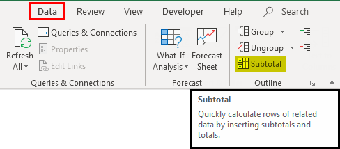
In all of the above examples, we have inserted our own subtotal rows with SUM formulas. To have subtotals calculated automatically, use the Subtotal command with the summary function of your choice such as SUM, COUNT, AVERAGE, MIN, MAX, etc. The Subtotal command will not only insert summary rows but also create an outline with collapsible and expandable rows, thus completing two tasks at once!
Apply default Excel styles to summary rows
Microsoft Excel has the predefined styles for two levels of summary rows: RowLevel_1 (bold) and RowLevel_2 (italic). You can apply these styles before or after grouping rows.
To automatically apply Excel styles to a new outline, go to the Data tab > Outline group, click the Outline dialog box launcher, and then select the Automatic styles check box, and click OK. After that you create an outline as usual. 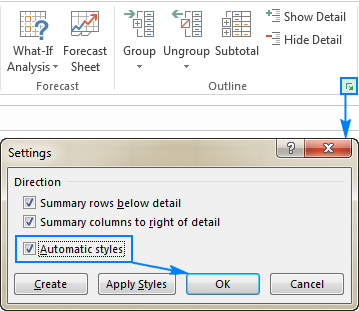
To apply styles to an existing outline, you also select the Automatic styles box as shown above, but click the Apply Styles button instead of OK.
Here’s how an Excel outline with the default styles for summary rows looks like: 
How to select and copy only visible rows
After you’ve collapsed irrelevant rows, you may want to copy the displayed relevant data somewhere else. However, when you select the visible rows in the usual way using the mouse, you are actually selecting the hidden rows as well.
To select only the visible rows, you’ll need to perform a few extra steps:
- Select visible rows using the mouse.
For example, we have collapsed all of the detail rows, and now select the visible summary rows: 

As the result, only the visible rows are selected (the rows adjacent to hidden rows are marked with a white border): 
And now, you simply press Ctrl + C to copy the selected rows and Ctrl + V to paste them wherever you like.
How to hide and show outline symbols
To hide or display the outline bars and level numbers in Excel, use the following keyboard shortcut: Ctrl + 8 .
Pressing the shortcut for the first time hides the outline symbols, pressing it again redisplays the outline.
The outline symbols don’t show up in Excel
If you can see neither the plus and minus symbols in the group bars nor the numbers at the top of the outline, check the following setting in your Excel:
- Go to the File tab >Options >Advanced category.
- Scroll down to the Display options for this worksheet section, select the worksheet of interest, and make sure the Show outline symbols if an outlineis applied box is selected.

This is how you group rows in Excel to collapse or expand certain sections of your dataset. In a similar fashion, you can group columns in your worksheets. I thank you for reading and hope to see you on our blog next week.
Источник
I do this all the time with vba. I am pretty sure I have used the same method since office 95′, with minor changes made for column placement. It can be done with fewer lines if you don’t define the variables. It can be done faster if you have a lot of lines to go through or more things that you need to define your group with.
I have run into situations where a ‘group’ is based on 2-5 cells. This example only looks at one column, but it can be expanded easily if anyone takes the time to play with it.
This assumes 3 columns, and you have to sort by the group_values column.
Before you run the macro, select the first cell you want to compare in the group_values column.
'group_values, some_number, empty_columnToHoldSubtotals
'(stuff goes here)
'cookie  1   empty
'cookie  3   empty
'cake    4   empty
'hat     0   empty
'hat     3   empty
'...
'stop
Sub subtotal()
  ' define two strings and a subtotal counter thingy
  Dim thisOne, thatOne As String
  Dim subCount As Double

  ' seed the values
  thisOne = ActiveCell.Value
  thatOne = ActiveCell.Offset(1, 0)
  subCount = 0

  ' setup a loop that will go until it reaches a stop value
  While (ActiveCell.Value <> "stop")

    ' compares a cell value to the cell beneath it.
    If (thisOne = thatOne) Then
      ' if the cells are equal, the line count is added to the subcount
      subCount = subCount + ActiveCell.Offset(0, 1).Value

    Else
      ' if the cells are not equal, the subcount is written, and subtotal reset.
      ActiveCell.Offset(0, 2).Value = ActiveCell.Offset(0, 1).Value + subCount
      subCount = 0

    End If

    ' select the next cell down
    ActiveCell.Offset(1, 0).Select

    ' assign the values of the active cell and the one below it to the variables
    thisOne = ActiveCell.Value
    thatOne = ActiveCell.Offset(1, 0)
  Wend

End Sub
Excel for Microsoft 365 Excel for Microsoft 365 for Mac Excel 2021 Excel 2019 Excel 2016 Excel 2013 Excel 2010 More…Less
In Power Query, you can group the same values in one or more columns into a single grouped row. You can group a column by using an aggregate function or group by a row.
Example
The following procedures are based on this query data example:
You can group data by using an aggregate function, such as Sum and Average. For example, you want to summarize the total units sold at the country and sales channel level, grouped by the Country and Sales Channel columns.
-
To open a query, locate one previously loaded from the Power Query Editor, select a cell in the data, and then select Query > Edit. For more information see Create, edit, and load a query in Excel.
-
Select Home > Group by.
-
In the Group by dialog box, select Advanced to select more than one column to group by.
-
To add another column, select Add Grouping.
Tip To delete or move a grouping, select More (…) next to the grouping name box.
-
Select the Country and Sales Channel columns.
-
In the next section:
New column name Enter «Total units» for the new column header.
Operation Select Sum. The aggregations available are Sum, Average, Median, Min, Max, Count Rows, and Count Distinct Rows.
Column Select Units to specify which column to aggregate.
-
Select OK.
Result
A Row Operation does not require a column, because data is grouped by a row in the Group By dialog box. There are two choices when you create a new column:
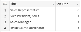
Count Rows
which displays the number of rows in each grouped row.
Procedure
For example, to group by all rows, you want the total units sold and you want two other columns that give you the name and units sold for the top-performing product, summarized at the country and sales channel level.
-
To open a query, locate one previously loaded from the Power Query Editor, select a cell in the data, and then select Query > Edit. For more information see Create, load, or edit a query in Excel.
-
Select Home > Group by.
-
In the Group by dialog box, select Advanced to select more than one column to group by.
-
Add a column to aggregate by selecting Add aggregation at the bottom of the dialog box.
Tip To delete or move an aggregation, select More (…) next to the column box.
-
Under Group by, select the Country and Sales Channel columns.
-
Create two new columns by doing the following:
Aggregation Aggregate the Units column by using the Sum operation. Name this column Total units.
All rows Add a new Products column by using the All rows operation. Name this column Total products. Because this operation acts upon all rows, you don’t need to make a selection under Column and so it is not available.
-
Select OK.
Result
See Also
Power Query for Excel Help
Grouping or summarizing rows (docs.com)
Need more help?
What Is Group In Excel?
The Group is an Excel tool that groups two or more rows or columns. With this function, the user has the option to minimize and maximize the grouped data. The rows or columns of the group collapse on minimizing and expand on maximizing. The group option is available under the Outline section of the Data tab.
You are free to use this image on your website, templates, etc, Please provide us with an attribution linkArticle Link to be Hyperlinked
For eg:
Source: Group in Excel (wallstreetmojo.com)
Table of contents
- What is Group in Excel?
- How to Group Data in Excel?
- Auto Outline With Succeeding Subtotals
- Auto Outline With Preceding Subtotals
- The Collapse and Expansion of Grouped Data
- Manual Grouping
- Automatic Subtotals
- Frequently Asked Questions
- Recommended Articles
- How to Group Data in Excel?
- The Group in excel is used to group two or more rows or columns.
- We can collapse or expand the grouped data by minimizing and maximizing, respectively.
- The Excel shortcut keys to group data are Shift+Alt+Right Arrow. Similarly, the shortcut keys to ungroup the grouped data are Shift+Alt+Left Arrow.
- The “clear outline” option removes grouping from the worksheet.
- When we are using the “auto outline” option while grouping, the subtotals can either precede or succeed the grouped data.
- Alternatively, we can also use the shortcut keys Shift+Alt+Left Arrow.
How to Group Data in Excel?
Let us consider a few examples.
Example #1 – Auto Outline With Succeeding Subtotals
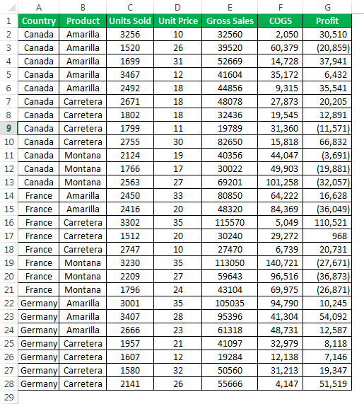
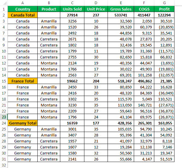
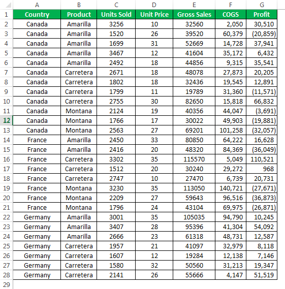
The Excel sheet consisting of the country name, product, units sold, price, gross sales, COGS, and profit is shown in the succeeding image. We can either club the countries into one or group the products into categories to make the data precise.
Let us go with the former approach and club the countries.
The steps to create an auto outline with succeeding subtotals are listed as follows:
- Enter the data as shown in the following image.

- To each country, add subtotals manually

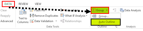
- Place the cursor inside the table. Click on Auto outline in Group under the Data tab.

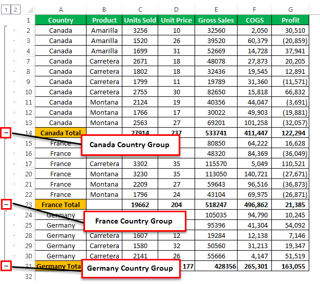
- Clicking on Auto Outline will group the range included in the country-wise total.

- Clicking the plus sign (+) hides the sub-items of each country. The consolidated summary of every country can be seen as highlighted in the below image.


Example #2 – Auto Outline With Preceding Subtotals
In the previous method, we added the totals at the end of every country. Let us add the totals before the data of a particular country.
The steps to group data with preceding totals are:
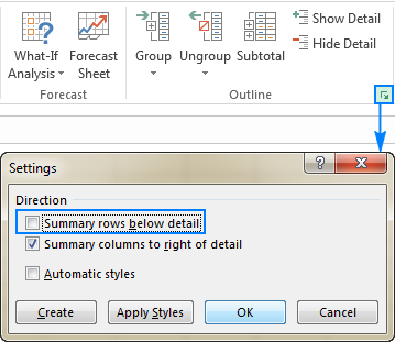
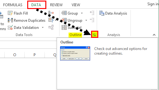
- Step 1: Click on the Dialog Box Launcher under the Outline section of the Data tab.
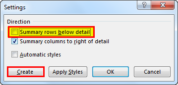
- Step 2: The Settings dialog box appears.
Uncheck the box Summary rows below detail and click on Create to complete the process.
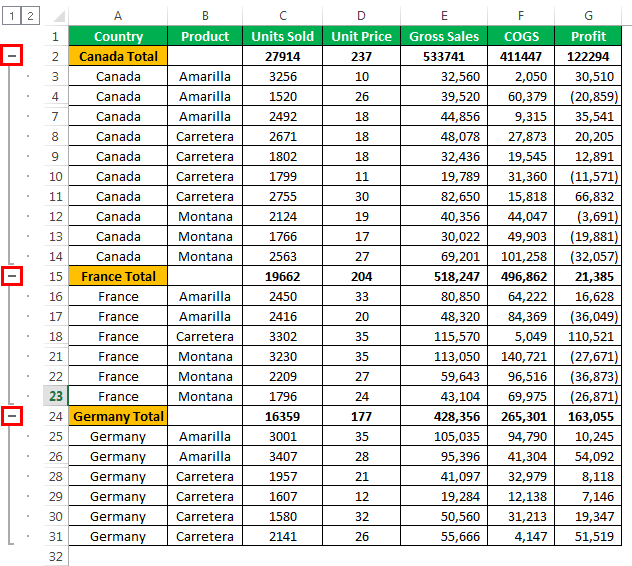
- Step 3: The group buttons appear at the top.
Example #3 – The Collapse And Expansion Of Grouped Data
At any point in time, we can collapse or expand the group. In the top left-hand corner, there are two numbers following the name box. The numbers 1 and 2 appear within the boxes.
Clicking on 1 reveals the group summary, as shown in the following image.
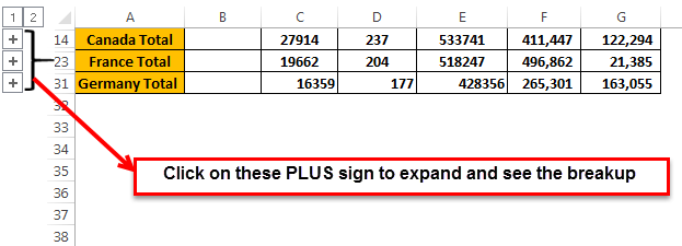
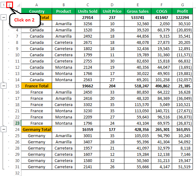
Clicking on 2 expands the table and reveals the breakup of the group, as shown below.
Example #4 – Manual Grouping
The previous examples utilize the basic Excel formulas and groups automatically. An alternative method is to group manually.
The steps for manual grouping are as follows:
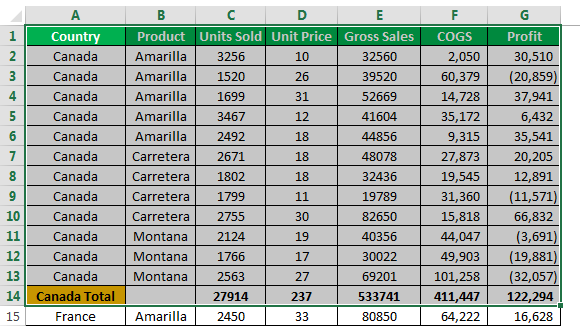
- Step 1: Select the range (row-wise) that we have to group. To group Canada, select the range till row 14.
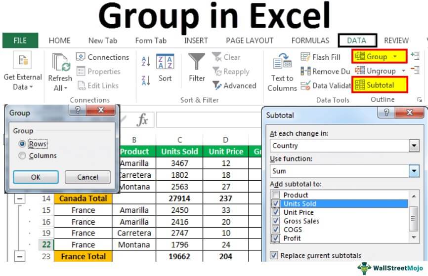
- Step 2: Select Group under the Data tab.
- Step 3: A dialog box, titled Group appears.
Since we are grouping the data row-wise, select “rows” option.
Alternatively, the Excel shortcut Shift+Alt+Right Arrow groups selected cells of the data.
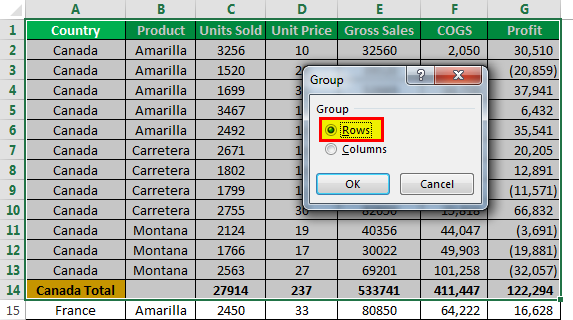
- Step 4: Now, we have grouped the rows of Canada.
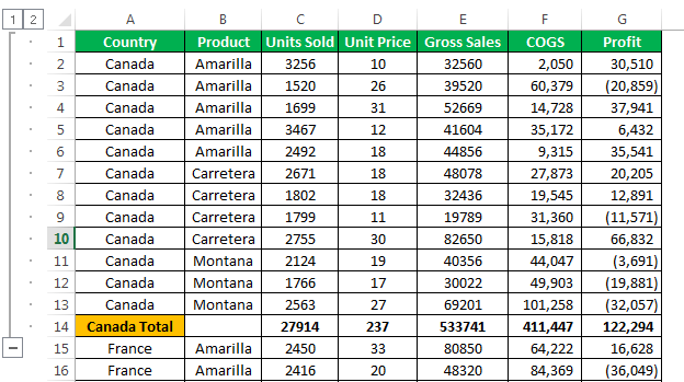
Remember, we have to repeat the process of manually grouping for the other countries as well. Please note that we should select the data of every country before grouping.
Note: The data should not contain any hidden rows during manual grouping.
Example #5 – Automatic Subtotals
In the previous examples, we added the subtotals manually. Alternatively, we can also add subtotals automatically.
The steps to add subtotals automatically are:
- Step 1: First, we should remove all the added subtotals manually.
- Step 2: Click on Subtotal under the Data tab.

- Step 3: The Subtotal dialog box appears.
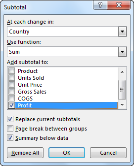
- Step 4: Select the basis on which subtotals are to be added.
- Select Country as the base, under At each change in: option.
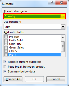
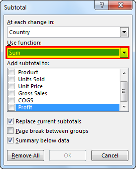
- Step 5: Since totals are required, select Sum under Use function: option.
Note: The user can select different functions like sum, average, min, max, etc., in the “subtotal” dialog box.
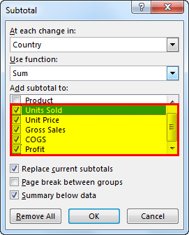
- Step 6: For totaling the columns, select them under Add subtotal to:. Check the boxes for Units Sold, unit price, Gross Sales, COGS, and Profit.
Click OK.
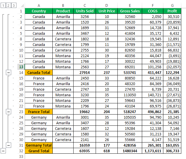
- Step 7: The subtotals and the groups appear, as shown below.
Important Things To Note
- Group in excel is used to group rows and columns.
- It is used to create structured financial models.
- Also, it helps to read complex data.
Frequently Asked Questions
1. What is group in Excel?
The Group in Excel is a tool that helps club similar data. It provides an organized, compact, and readable view to the reader. For grouping, the worksheet must contain headings and subtotals for every column and row respectively. Moreover, there should not be any blank cells in the data to be grouped.
The groups in Excel are used to create structured financial models. Since groups provide minimize and maximize options, they are used to hide unnecessary calculations.
2. Why is data grouped and ungrouped in Excel?
The data is grouped and ungrouped for the following reasons:
• Grouping helps read through the detailed and complex data. Ungrouping removes the grouping of rows and columns, thereby helping the user go back to the initial data view.
• With grouping, it is possible to look at the required data sections of the worksheet. Ungrouping helps to look at the entire worksheet data in one go.
Note: The grouping shortcut is Shift+Alt+Right Arrow, and the ungrouping shortcut is Shift+Alt+Left Arrow.
3. How does ungrouping work in Excel?
The ungrouping of data works as follows:
• To ungroup the entire data, clear the outline.
Click Clear outline under the Ungroup arrow (Outline section of the Data tab).
• To ungroup particular data, select the rows to be ungrouped. In the ungroup box, select Rows option and click OK.
Alternatively, we can also use the shortcut keys Shift+Alt+Left Arrow.
Note: Ungrouping does not delete any data. In case the outline is removed, it cannot be undone with Ctrl+Z.
Download Template
This article must be helpful to understand the Group in Excel, with its formula and examples. You can download the template here to use it instantly.
You can download this Group in Excel template here – Group in Excel template
Recommended Articles
This has been a guide to Group in Excel (Auto, Manual). Here we discuss how to group and ungroup data in Excel along with examples and downloadable Excel template. You may learn more about Excel from the following articles –
- Group Rows in Excel
- ExcelGroup Data
- Group Excel Worksheets
- Excel Column Grouping
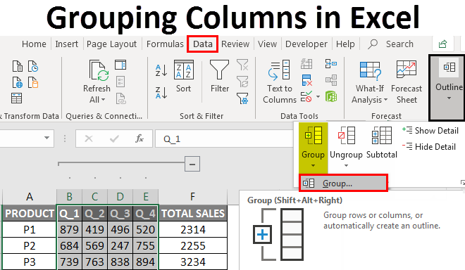
Grouping Columns in Excel (Table of Content)
- Excel Grouping Columns
- How to Enable Grouping of Columns in Excel?
Excel Grouping Columns
Sometimes the worksheet contains complex data, which is very difficult to read & analyze, to Access & read these types of data in an easier way, the grouping of cells will help you out. Grouping of columns or rows is used if you want to visually group of items or to monitor them in a concise & organized manner under one heading or if you want to hide or show data for better display & presentation. Grouping is very useful & most commonly used in accounting & finance spreadsheets. Under the Data tab in the Ribbon, you can find the Group option in the outline section. In this topic, we are going to learn about Grouping Columns in Excel.
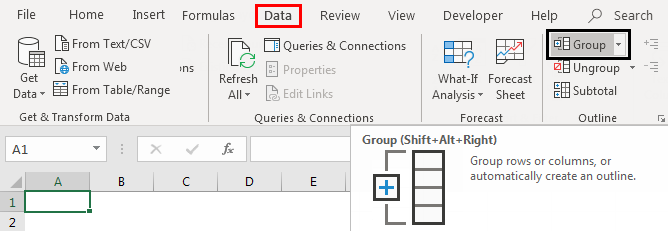
Shortcut Key to Group Columns or Rows
Shift+Alt+Right Arrow is the shortcut key to group columns or rows, whereas
Shift+Alt+Left Arrow is the shortcut key to ungroup columns or rows.
Definition Grouping of Columns in Excel
It’s a process where you visually group the column items or datasets for a better display.
How to Enable Grouping of Columns in Excel?
Let’s check out how to group columns & How to collapse & expand columns after grouping columns.
You can download this Grouping Columns Excel Template here – Grouping Columns Excel Template
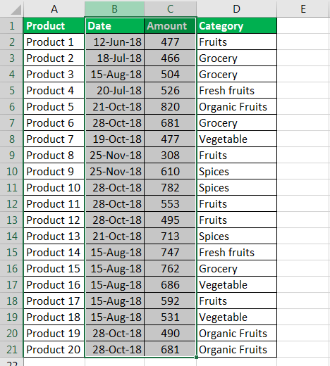
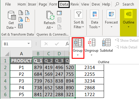
Example #1 – Grouping of Columns in Excel
Grouping of columns in Excel works out well for structured data where it should contain column headings, and it should not have a blank column or row data.
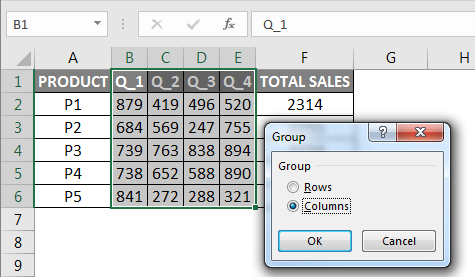
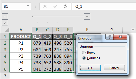
Initially, you need to select the column in which you want to group it (i.e. B, C, D, E columns). Go to the Data tab, then click on the group option under the outline section.
Click on the columns and then press OK.
Now you can observe in data, the columns are grouped perfectly, and the outline bars you can observe at the top represent different levels of data organization. Grouping also introduces a toggle option, or it will create a hierarchy of groups, which is known as an outline, to help your worksheet appear in an organized manner, where each bar represents a level of organization (Grouping is also referred to as Outlines.)
How to Collapse & Expand Columns After Column Grouping
you can press the “-” buttons in the margin to collapse the columns (B, C, D, E Columns completely disappears) or in case If you want to expand them again, press the “+” buttons in the margin (B, C, D, E Columns appears)
Another way to access data is the use of 1 or 2 options on the left side of the worksheet, i.e. it is called a state, 1st option is called a hidden state (if you click on it, it will hide B, C, D, E Columns) whereas 2nd option is called unhidden state, it will expand those hidden columns, I.E. B, C, D, E Columns appears
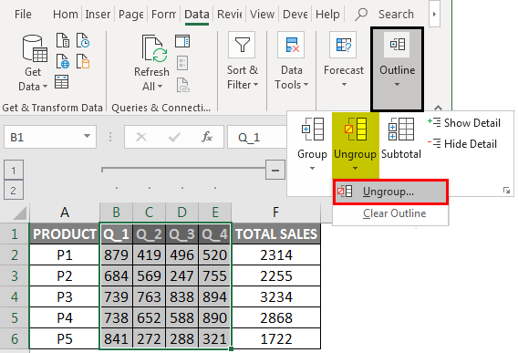
To Ungroup Columns in Excel
Select the columns you wish to ungroup (i.e. the columns which you have previously grouped). On the Data tab, in the Outline group, click on Ungroup command.
Click on the columns and then press OK.
Now, you can observe data bars & “+” buttons and “-” buttons disappear in the excel sheet once the ungroup option is selected.
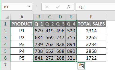
Example #2 – Multiple Grouping of Columns for Sales Data in Excel
In the below-mentioned example, the Table contains product monthly sales data from Jan to Dec month, and it is also represented in quarterly & yearly sales.
Here the data is structured and does not contain any blank cells, hidden rows, or columns.
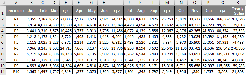
I don’t want all the monthly sales data to be displayed; I want only quarterly & yearly sales data to be displayed; it can be done through multiple grouping of column options.
Initially, I need to select the column which I want to group it; now, let’s select the months (i.e. Jan, Feb, Mar columns). Go to the Data tab in the Home ribbon, and it will open a toolbar below the ribbon, then click on the group option under the outline section; now you can observe in a data, the columns are grouped perfectly.
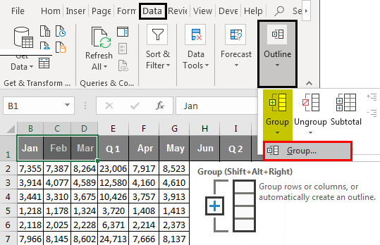
Click on the columns and then press OK.
A similar procedure is applied or followed for the month of Apr, May, Jun & Jul, Aug, Sep & Oct, Nov, Dec columns.
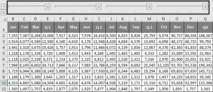
Once the grouping of the above-mentioned monthly columns is done, you can observe that the columns are grouped perfectly in a dataset. The four outline bars you can observe at the top represent different data organisation levels.
Collapsing & Expanding Columns After Column Grouping
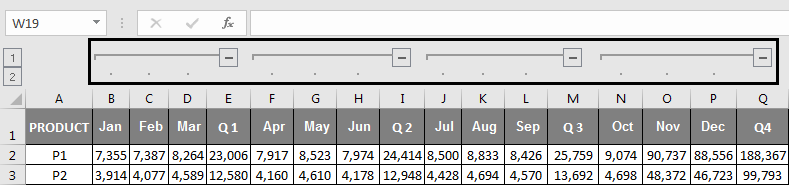
You can press the “–” symbol or buttons in the outline bar to collapse all the month columns; once you are done, you can observe all the month Columns completely disappears, and Positive or “+” buttons in the outline bar appear.

Now, the sales data looks in a concise & compact form, and it looks well-organized & structured financial data. In case if you want to check any specific monthly sales data, you can expand them again by pressing the “+” buttons in in outline bar so that again, all the monthly sales data will appear.
Another way to access or hide monthly data is the use of 1 or 2 options on the left side of the worksheet, i.e. it is called a state, 1st option is called a hidden state (On a single click on it, it will hide all the month Columns) whereas 2nd option is called unhidden state, it will expand those hidden columns, I.E. all the month Columns appears.
Things to Remember
Grouping columns or rows in Excel is useful to create and maintain well-organized and well-structured financial sales data.
It is a better & superior alternative for hiding & unhiding cells; sometimes, it is not clear to the other user of the excel spreadsheet if you use the hide option. He needs to track which columns or rows you have hidden & where you have hidden.
Prior to applying grouping of columns or rows in excel, You have to ensure that your structured data should not contain any hidden or blank rows & columns; otherwise, your data will be grouped incorrectly.
Apart from grouping, you can also do summarization of datasets in different groups with the help of the Subtotal command.
Recommended Articles
This has been a guide to Grouping Columns in Excel. Here we discussed How to Enable Grouping of Columns in Excel along with Examples and a downloadable excel template. You may also look at these useful functions in excel –
- Excel Move Columns
- VBA Columns
- Freeze Columns in Excel
- Switching Columns in Excel