Google excel if statement - Word и Excel - помощь в работе с программами

Возвращает различные значения в зависимости от результата логической проверки (ИСТИНА или ЛОЖЬ).

Пример использования

ЕСЛИ(A2 = "а"; "A2 это а")

ЕСЛИ(A2; "A2 было истиной"; "A2 было ложью")

ЕСЛИ(ИСТИНА; 4; 5)

Синтаксис

ЕСЛИ(источник; значение_при_соблюдении_условия; значение_при_несоблюдении_условия)

источник – логическое значение или адрес ячейки, содержащей такое значение (то есть ИСТИНА или ЛОЖЬ).
значение_при_соблюдении_условия – возвращается функцией, если источник соответствует логическому значению ИСТИНА.
значение_при_несоблюдении_условия (необязательно, по умолчанию отсутствует) – возвращается функцией, если источник соответствует логическому значению ЛОЖЬ.

Примечания

Большинство ошибок, возникающих при использовании функции ЕСЛИ, связаны с неверным порядком аргументов значение_при_соблюдении_условия и значение_при_несоблюдении_условия. Уделите ему особое внимание.

Примеры

Ниже показано, как функция используется для проведения логической проверки.

Эта информация оказалась полезной?

Как можно улучшить эту статью?

Источник

11.11.2022

Функция IF (ЕСЛИ) в Google таблицах — на практике одна из самых востребованных. В зависимости от условий она возвращает указанный результат (значение или другую формулу со своими параметрами).

Новички без особых знаний (математика за 3 класс) с помощью данной функции могут построить простые отчеты, которые уже будут удовлетворять потребности в визуальном восприятии результата работы.

Функция IF (ЕСЛИ) в Google таблицах

Логическая функция имеет следующий синтаксис:

 =IF(логическое_выражение; значение_если_истина; [значение_если_ложь])

Логическое_выражение – это искомое проверяемое условие. Например: B2<100. Если значение в ячейке B2 действительно меньше 100, то в памяти гугл таблиц генерируется ответ «ИСТИНА» и функция возвращает то, что указано следующим параметром. Если это не так, в памяти генерируется ответ «ЛОЖЬ» и возвращается значение из последнего указанного нами параметра.

Значение_если_истина – значение или любая другая формула, которая отображается при наступлении указанного в первом параметре события.
[Значение_если_ложь] – это альтернативное значение или любая другая формула, которая отображается при невыполнении нашего условия (первый проверяемый параметр). Данный параметр не обязателен к заполнению. В этом случае при наступлении альтернативного события функция вернет значение «ЛОЖЬ». Для удобства все необязательные к заполнению параметры в формулах google таблиц помечаются в квадратными скобками «[…]».

Примеры функции IF (ЕСЛИ) в Google таблицах

Функция IF (ЕСЛИ) практически всегда используется в связке с другими функциями. Чаще всего она является составным элементом в сложной аналитической структуре. Но ее можно использовать и в простейших вариантах.

Простой пример функции IF (ЕСЛИ)

Рассмотрим очень простой пример проверки продаж отдельных продуктов. По условию, нам нужно пометить, какие продукты хорошо продаются, а какие нет. Критерий определения — больше 30 кг в день. Если в день мы продаем больше 30 кг — Хорошо, если меньше — Плохо.

В таком случае синтаксис формулы будет выглядеть так:

 =IF(логическое_выражение; значение_если_истина; [значение_если_ложь])

 =IF(B2>30;"Хорошо";"Плохо")

Все текстовые выражения помещаются в кавычки (слова, числа в виде текста и т.д.).

Пошагово: IF (ЕСЛИ) мы продали моркови больше 30 кг за 1 день, то выводится значение_если_истина — «Хорошо» (да, мы продали 35 кг > 30 кг), если меньше — «Плохо» ([значение_если_ложь] — альтернативное значение, если условие не соблюдается).

Более сложный пример функции IF (ЕСЛИ)

Допустим, у нас на складе есть определенное количество овощей и нам нужно рассчитать сколько товаров останется после недели торговли. Для этого нам нужно умножить значения дневных продаж на 7 (дни недели), а зачем вычесть полученный результат из имеющихся складских остатков.

 =C2-B2*7

Мы столкнулись с ситуацией, когда математический результат продаж наших товаров оказался отрицательным, а все понимают, что остатков на складе не может быть меньше нуля. Чтобы прогноз был корректным, нужно заменить отрицательные значения нулями. С такой задачей прекрасно справится функция IF (ЕСЛИ). Она проверит результат вычислений и если он окажется меньше нуля — выдаст ответ «0», а если больше — отобразит результат вычислений.

 =IF(логическое_выражение; значение_если_истина; [значение_если_ложь])

 =IF(C2-B2*7<0;0;C2-B2*7)

Таким образом мы получили корректный результат и в прогнозе нет больше отрицательных значений.

Функция IF (ЕСЛИ) в Google таблицах — несколько условий

Чаще всего на практике требуется применять формулу где условий более чем 2 — 3, 4, 5… В таком случае можно использовать функцию, но уже вкладывая одну в одну, как матрешку, указывая все условия по очереди.

Рассмотрим пример многомерной функции IF (ЕСЛИ) на живом примере начисления премии по KPI продаж. Система начислений следующая:

Если план выполнен менее чем на 90% — премия не начисляется.
90% — 95% — премия 10%.
95% — 100% — премия 20%.
Если план перевыполнен — премия 30%.

Фактически у нас 4 конкретных условия, которые могут быть указаны по следующей логической структуре:

если выполняется первое условие, то выводится первый вариант, в противном случае переход ко второму условию;
если выполняется второе условие, то выводится второй вариант, в противном случае переход к третьему условию;
если выполняется третье условие, то выводится третий вариант, в противном случае переход к четвертому условию;
если выполняется четвертое условие, то выводится четвертый вариант, а в качестве завершения логической структуры указывается [Значение_если_ложь].

Максимальное количество таких условий = 256. В конце формулы указывается [Значение_если_ложь], для которого не выполняется ни одно из перечисленных ранее условий. В итоге формула имеет следующий синтаксический вид:

 =IF(логическое_выражение; значение_если_истина; IF(логическое_выражение; значение_если_истина; IF(логическое_выражение; значение_если_истина; [Значение_если_ложь])))

 =IF(B2<0,9;0;IF(B2<0,95;0,1;IF(B2<1;0,2;0,3)))

Цветом выделены 4 условия, по которым формула выводит результат заданной функции. Важно понимать, что комбинация функций IF (ЕСЛИ) работает так, что при выполнении какого-либо указанного условия — следующие уже не проверяются. Поэтому их нужно указать в правильной последовательности.

При создании формульной логической цепочки очень легко запутаться. Новичкам рекомендуется либо абстрактно принимать переменные (условия) за «Х», «Y», «Z», …, либо смотреть на всплывающие подсказки. Плюсом, система сама подсвечивает разные переменные и условия, а так же, доставляет закрывающие скобки формулы функций.

Функция IFS (ЕСЛИМН) в Google таблицах

В более поздних версиях Excel и Google таблицах (с 2016 года) появилась функция IFS (ЕСЛИМН). Она фиксирует сразу множество условий, что значительно оптимизирует серверную нагрузку (формулы считаются быстрее и наши таблицы не тормозят так, как это было бы, если бы сервер просчитывал каждое вложенное условие IF (ЕСЛИ)) и разгружает наше абстрактное мышление, упраздняя повторяющиеся простые условия IF (ЕСЛИ). По сути, это та же функция ЕСЛИ, только в разы упрощенная, к тому же, максимальное число условий увеличилось до 512.

В качестве примера возьмем имеющиеся значения из примеров выше и рассчитаем начисление премий уже более простой, но не менее функциональной функцией:

Первый вариант

 =IFS(B2<0,9;0;B2<0,95;0,1;B2<1;0,2;B2>=1;0,3)

Второй вариант

 =IFS(B2<0,9;0;B2<0,95;0,1;B2<1;0,2;TRUE;0,3)

Формулы функции IFS (ЕСЛИМН) выполняют одно и то же действие, отличаясь завершающим последним обязательным (в отличии от обычной функции IF (ЕСЛИ)) аргументом. В первом варианте мы конкретно указали какое значение у аргумента должно выводиться, если выполняется 4 условие функции. Можно избежать конкретного действия, прописав значение «TRUE» (ИСТИНА), тогда будет выводиться последнее альтернативное значение 4 условия.

P.S.: первый вариант мне нравится больше.

Вы познакомились с функциями IF (ЕСЛИ) и IFS (ЕСЛИМН), увидели где их можно применить на практике, и, я уверен, сможете применить их в своей работе. Поделитесь, пожалуйста в комментариях своими идеями или случаями применения рассматриваемых функций.

Источник

This tutorial demonstrates how to use the IF Function in Excel and Google Sheets to create If Then Statements.

IF Function Overview

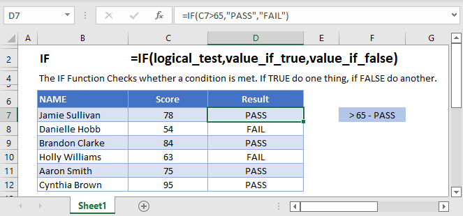
The IF Function Checks whether a condition is met. If TRUE do one thing, if FALSE do another.

How to Use the IF Function

Here’s a very basic example so you can see what I mean. Try typing the following into Excel:

=IF( 2 + 2 = 4,"It’s true", "It’s false!")

Since 2 + 2 does in fact equal 4, Excel will return “It’s true!”. If we used this:

=IF( 2 + 2 = 5,"It’s true", "It’s false!")

Now Excel will return “It’s false!”, because 2 + 2 does not equal 5.

Here’s how you might use the IF statement in a spreadsheet.

=IF(C4-D4>0,C4-D4,0)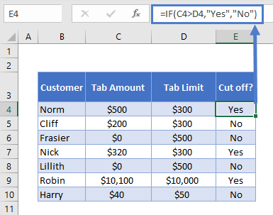

You run a sports bar and you set individual tab limits for different customers. You’ve set up this spreadsheet to check if each customer is over their limit, in which case you’ll cut them off until they pay their tab.

You check if C4-D4 (their current tab amount minus their limit), is greater than 0. This is your logical test. If this is true, IF returns “Yes” – you should cut them off. If this is false, IF returns “No” – you let them keep drinking.

What can IF Return?

Above we returned a text string, “Yes” or “No”. But you can also return numbers, or even other formulas.

Let’s say some of your customers are running up big tabs. To discourage this, you’re going to start charging interest on customers who go over their limit.

You can use IF for that:

=IF(C4>D4,C4*0.03,0)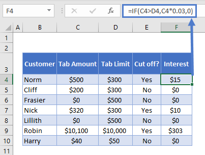

If the tab is higher than the limit, return the tab multiplied by 0.03, which returns 3% of the tab. Otherwise, return 0: they aren’t over their tab, so you won’t charge interest.

Using IF with AND

You can combine IF with Excel’s AND Function to test more than one condition. Excel will only return TRUE if ALL of the tests are true.

So, you implemented your interest rate. But some of your regulars are complaining. They’ve always paid their tabs in the past, why are you cracking down on them now? You come up with a solution: you won’t charge interest to certain trusted customers.

You make a new column to your spreadsheet to identify trusted customers, and update your IF statement with an AND function:

=IF(AND(C4>D4, F4="No"),C4*0.03,0)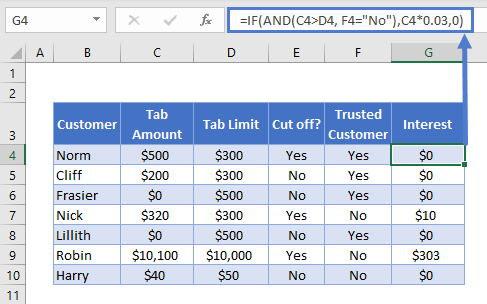

IF AND

Let’s look at the AND part separately:

AND(C4>D4, F4="No")

Note the two conditions:

C4>D4: checking if they’re over their tab limit, as before
F4=”No”: this is the new bit, checking if they are not a trusted customer

So now we only return the interest rate if the customer is over their tab, AND we have “No” in the trusted customer column. Your regulars are happy again.

Using IF with OR

The OR Function allows you to test more than one condition, returning TRUE if any conditions are met.

Maybe customers being over their tab is not the only reason you’d cut them off. Maybe you give some people a temporary ban for other reasons, gambling on the premises perhaps.

So you add a new column to identify banned customers, and update your “Cut off?” column with an OR test:

=IF(OR(C4>D4,E4="Yes"),"Yes","No")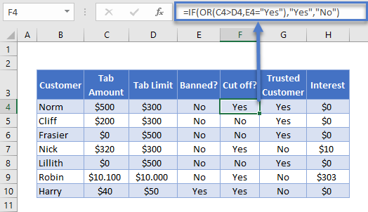

Looking just at the OR part:

OR(C4>D4,E4="Yes")

There are two conditions:

C4>D4: checking if they’re over their tab limit
F4=”Yes”: the new part, checking if they are currently banned

This will evaluate to true if they are over their tab, or if there is a “Yes” in column E. As you can see, Harry is cut off now, even though he’s not over his tab limit.

Using IF with XOR

The XOR Function returns TRUE if only one condition is met. If more than one condition is met (or not conditions are met). It returns FALSE.

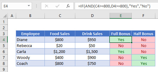
An example might make this clearer. Imagine you want to start giving monthly bonuses to your staff :

If they sell over $800 in food, or over $800 in drinks, you’ll give them a half bonus
If they sell over $800 in both, you’ll give them a full bonus
If they sell under $800 in both, they don’t get any bonus.

You already know how to work out if they get the full bonus. You’d just use IF with AND, as described earlier.

=IF(AND(C4>800,D4>800),"Yes","No")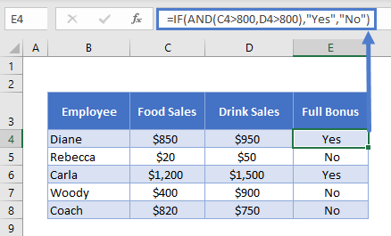

But how would you work out who gets the half bonus? That’s where XOR comes in:

=IF(XOR(C4>=800,D4>=800),"Yes","No")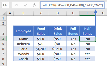

As you can see, Woody’s drink sales were over $800, but not food sales. So he gets the half bonus. The reverse is true for Coach. Diane and Carla sold more than $800 for both, so they don’t get a half bonus (both arguments are TRUE), and Rebecca made under the threshold for both (both arguments FALSE), so the formula again returns “No”.

Using IF with NOT

The NOT Function reverses the outcome of a logical test. In other words, it checks whether a condition has not been met.

You can use it with IF like this:

=IF(AND(C3>=1985,NOT(D3="Steven Spielberg")),"Watch", "Don’t Watch")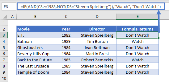

IF NOT

Here we have a table with data on some 1980s movies. We want to identify movies released on or after 1985, that were not directed by Steven Spielberg.

Because NOT is nested within an AND Function, Excel will evaluate that first. It will then use the result as part of the AND.

Nested IF Statements

You can also return an IF statement within your IF statement. This enables you to make more complex calculations.

Let’s go back to our customers table. Imagine you want to classify customers based on their debt level to you:

$0: None
Up to $500: Low
$500 to $1000: Medium
Over $1000: High

You can do this by “nesting” IF statements:

=IF(C4=0,"None",IF(C4<=500,"Low",IF(C4<=1000,"Medium",IF(C4>1000,"High"))))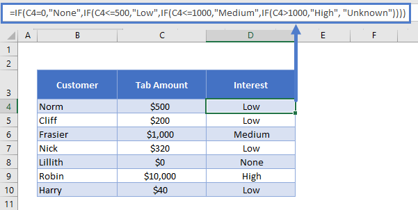

It’s easier to understand if you put the IF statements on separate lines (ALT + ENTER on Windows, CTRL + COMMAND + ENTER on Macs):

=
IF(C4=0,"None",
IF(C4<=500,"Low",
IF(C4<=1000,"Medium",
IF(C4>1000,"High", "Unknown"))))

IF C4 is 0, we return “None”. Otherwise, we move to the next IF statement. IF C4 is equal to or less than 500, we return “Low”. Otherwise, we move on to the next IF statement… and so on.

Simplifying Complex IF Statements with Helper Columns

If you have multiple nested IF statements, and you’re throwing in logic functions too, your formulas can become very hard to read, test, and update.

This is especially important to keep in mind if other people will be using the spreadsheet. What makes sense in your head, might not be so obvious to others.

Helper columns are a great way around this issue.

You’re an analyst in the finance department of a large corporation. You’ve been asked to create a spreadsheet that checks whether each employee is eligible for the company pension.

Here’s the criteria:

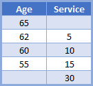
So if you’re under the age of 55, you need to have 30 years’ service under your belt to be eligible. If you’re aged 55 to 59, you need 15 years’ service. And so on, up to age 65, where you’re eligible no matter how long you’ve worked there.

You could use a single, complex IF statement to solve this problem:

=IF(OR(F4>=65,AND(F4>=62,G4>=5),AND(F4>=60,G4>=10),AND(F4>=55,G4>=15),G4>30),"Eligible", "Not Eligible")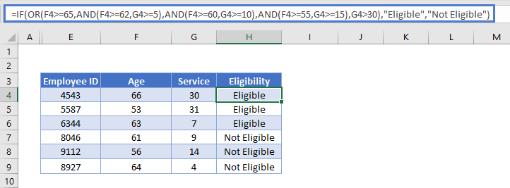

Whew! Kinda hard to get your head around that, isn’t it?

A better approach might be to use helper columns. We have five logical tests here, corresponding to each row in the criteria table. This is easier to see if we add line breaks to the formula, as we discussed earlier:

=IF(
OR(
F4>=65,
AND(F4>=62,G4>=5),
AND(F4>=60,G4>=10),
AND(F4>=55,G4>=15),
G4>30
),"Eligible","Not Eligible")

So, we can split these five tests into separate columns, and then simply check whether any one of them is true:

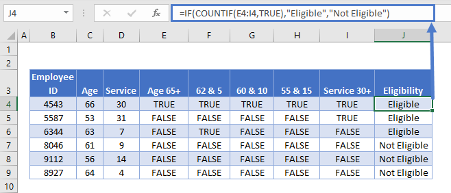
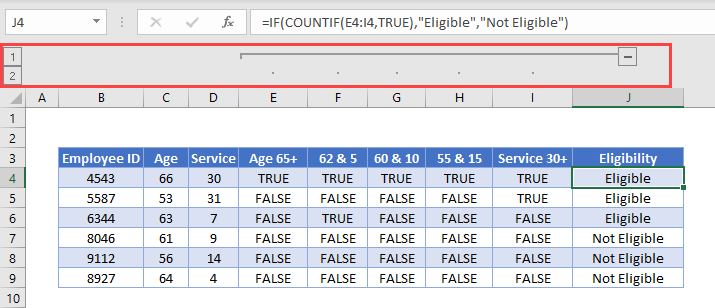
Each column in the table from E to I holds each of our criteria separately. Then in J4 we have the following formula:

=IF(COUNTIF(E4:I4,TRUE),"Eligible","Not Eligible")

Here we have an IF statement, and the logical test uses COUNTIF to count the number of cells within E4:I4 that contain TRUE.

If COUNTIF doesn’t find a TRUE value, it will return 0, which IF interprets as FALSE, so the IF returns “Not Eligible”.

If COUNTIF does find any TRUE values, it will return the number of them. IF interprets any number other than 0 as TRUE, so it returns “Eligible”.

Splitting out the logical tests in this way makes the formula easier to read, and if something’s going wrong with it, it’s much easier to spot where the mistake is.

Using Grouping to Hide Helper Columns

Helper columns make the formula easier to manage, but once you’ve got them in place and you know they are working correctly, they often just take up space on your spreadsheet without adding any useful information.

You could hide the columns, but this can lead to problems because hidden columns are hard to detect, unless you look closely at the column headers.

A better option is grouping.

Select the columns you want to group, in our case E:I. Then press ALT + SHIFT + RIGHT ARROW on Windows, or COMMAND + SHIFT + K on Mac. You can also go to the “Data” tab on the ribbon and select “Group” from the “Outline” section.

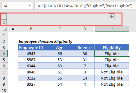
You’ll see the group displayed above the column headers, like this:

Then simply press the “-“ button to hide the columns:

The IFS Function

Nested IF statements are very useful when you need to perform more complex logical comparisons, and you need to do it in one cell. However, they can get complicated as they get longer, and they can be hard to read and update on your screen.

From Excel 2019 and Excel 365, Microsoft introduced another function, the IFS Function, to help make this a bit easier to manage. The nested IF example above could be achieved with IFS like this:

=IFS(
C4=0,"None",
C4<=500,"Low",
C4<=1000,"Medium",
C4>1000,"High",
TRUE, "Unknown",
)

You can read all about it on the main page for the Excel IFS Function <<link>>.

Using IF with Conditional Formatting

Excel’s Conditional Formatting feature enables you to format a cell in different ways depending on its contents. Since the IF returns different values based on our logical test, we might want to use Conditional Formatting with the IF Function to make these different values easier to see.

So let’s go back to our staff bonus table from earlier.

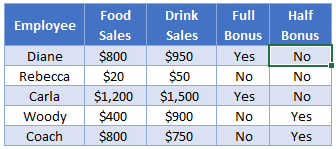
We’re returning “Yes” or “No” depending on what bonus we want to give. This tells us what we need to know, but the information doesn’t jump out at us. Let’s try to fix that.

Here’s how you’d do it:

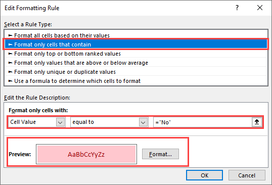
Select the cell range containing your IF statements. In our case that’s E4:F8.
Click “Conditional Formatting” on the “Styles” section of the “Home” tab on the ribbon.
Click “Highlight Cells Rules” and then “Equal to”.
Type “Yes” (or whatever return value you need) into the first box, and then choose the formatting you want from the second box. (I’ll choose green for this).
Repeat for all your return values (I’ll also set “No” values to red)

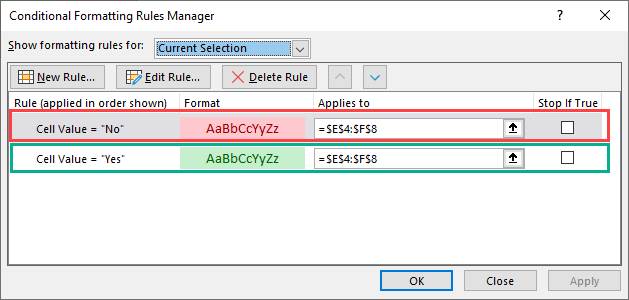
Here’s the result:

Using IF in Array Formulas

An array is a range of values, and in Excel arrays are represented as comma separated values enclosed in braces, such as:

{1,2,3,4,5}

The beauty of arrays, is that they enable you to perform a calculation on each value in the range, and then return the result. For example, the SUMPRODUCT Function takes two arrays, multiplies them together, and sums the results.

So this formula:

=SUMPRODUCT({1,2,3},{4,5,6})

…returns 32. Why? Let’s work it through:

1 * 4 = 4
2 * 5 = 10
3 * 6 = 18

4 + 10 + 18 = 32

We can bring an IF statement into this picture, so that each of these multiplications only happens if a logical test returns true.

For example, take this data:

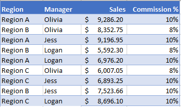
If you wanted to calculate the total commission for each sales manager, you’d use the following:

=SUMPRODUCT(IF($C$2:$C$10=$G2,$D$2:$D$10*$E$2:$E$10))

Note: In Excel 2019 and earlier, you have to press CTRL + SHIFT + ENTER to turn this into an array formula.

We’d end up with something like this:

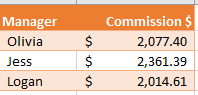
Breaking this down, the “Manager” column is column C, and in this example, Olivia’s name is in G2.

So the logical test is:

$C$2:$C$10=$G2

In English, if the name in column C is equal to what’s in G2 (“Olivia”), DO multiply the values in columns D and E for that row. Otherwise, don’t multiply them. Then, sum all the results.

You can learn more about this formula on the main page for the SUMPRODUCT IF Formula.

IF in Google Sheets

The IF Function works exactly the same in Google Sheets as in Excel:

VBA IF Statements

You can also use If Statements in VBA. Click the link to learn more, but here is a simple example:

Sub Test_IF ()

If Range("a1").Value < 0 then
  Range("b1").Value = "Negative"
End If

End Sub

This code will test if a cell value is negative. If so, it will write “negative” in the next cell.

Источник

IF is a Google Sheets function that acts based on a given condition. You provide a boolean and tell what to do based on whether it’s TRUE or FALSE. You can combine IF with other logical functions – AND, OR – to create nested formulas and go over multiple sets of criteria. But should you? IFS is a dedicated function, which evaluates multiple conditions to return a value. However, sometimes nested IF statements do better than IFS. Let’s explore some real-life examples and find out which logical function is a go.

If you prefer watching to reading, check out this simple tutorial by Railsware Product Academy on how to use the IF function (IFS, Nested IFs) in Google Sheets.

IF Google Sheets function explained

IF Google Sheets syntax

=IF(logical_expression, value_if_true, value_if_false)

IF function in Google Sheets evaluates one logical expression and returns a value depending on whether the expression is true or false. value_if_false is blank by default.

Google Sheets IF formula example

Interpretation of the Google Sheets IF formula:

If the value in the D1 cell equals one (logical_expression), then the formula will count the sum of values in the range B2:B (value_if_true). Otherwise, the formula will return an empty cell (value_if_false).

Nested IF Google Sheets statements for multiple logical expressions

Let’s say you need to evaluate multiple logical expressions. For this, you can nest multiple IF statements Google Sheets in a single formula. It may look as follows:

=IF(logical_expression#1, value_if_true,
IF(logical_expression#2, value_if_true, 
IF(logical_expression#3, value_if_true, 
IF(logical_expression#4,value_if_true,value_if_false))))

Example of a nested IF formula Google Sheets

=IF(D1>0, SUM(B2:B), IF(D1=0, "Nothing", IF(D1<0, AVERAGE(B2:B))))

Interpretation of the nested IF Google Sheets formula:

If the value in the D1 cell is above zero (logical_expression#1), then the formula will return the sum of values in the range B2:B (value_if_true); if the D1 cell is empty or its value is zero (logical_expression#2), then the formula will return “Nothing” (value_if_true); if the value in the D1 cell is below zero (logical_expression#3), then the formula will return the average of values in the range B2:B (value_if_true).

Nested IF statements can be improved with other logical functions: AND and OR.

IF + AND/OR Google Sheets for multiple logical expressions

AND and OR Google Sheets functions explained

	AND function	OR function
Returns TRUE	If all of the provided logical expressions are logically true*	If any of the provided logical expressions is logically true
Returns FALSE	If any of the provided logical expressions is logically false	If all of the provided logical expressions are logically false
Syntax	`=AND(logical_expression1, [logical_expression2, ...])`	`=OR(logical_expression1, [logical_expression2, ...])`

* All numbers (including negative ones) are logically true. The number 0 is logically false.

Let’s combine AND/OR with IF and check out how this works:

IF+AND Google Sheets formula example

=IF(AND(D1>0,D2>0,D3>0),SUM(B2:B),"Nothing")

Interpretation of the IF AND Google Sheets formula:

If the values in the cells D1 (logical_expression#1), D2 (logical_expression#2), and D3 (logical_expression#3) are above zero, then the formula will return the sum of values in the range B2:B (value_if_true). Otherwise, if any of the logical expressions is false, the formula will return “Nothing” (value_if_false).

IF+OR Google Sheets formula example

=IF(OR(D1>0,D2>0,D3>0),SUM(B2:B),"Nothing")

Interpretation of the IF OR Google Sheets formula:

If the value in the cell D1 (logical_expression#1), or D2 (logical_expression#2), or D3 (logical_expression#3) is above zero, then the formula will return the sum of values in the range B2:B (value_if_true). Otherwise, if all of the logical expressions are false, the formula will return “Nothing” (value_if_false).

IF+AND+OR formula Google Sheets example

=IF(OR(AND(D1>0,D2>0),AND(E1<0,E2<0)),SUM(B2:B),"Nothing")

Interpretation of the IF AND OR Google Sheets formula:

If the values in cells D1 and D2 are above zero (logical_expression#1), or the values in cells E1 and E2 are below zero (logical_expression#2), then the formula will return the sum of values in the range B2:B (value_if_true). Otherwise, if all of the logical expressions are false, the formula will return “Nothing” (value_if_false).

Logical operators (AND and OR) let you include versatile conditions in your IF formula. Keep in mind that AND/OR don’t work in arrays. Besides, multiple IF statements can be quite difficult to build and maintain. An alternative solution is to go with the IFS function.

IFS Google Sheets function explained

IFS Google Sheets syntax

=IFS(logical_expression#1, value_if_true, logical_expression#2, value_if_true, logical_expression#3, value_if_true,...)

IFS Google Sheets function evaluates multiple logical expressions and returns the first true value. If all the logical expressions are false, the function returns #N/A.

IFS Google Sheets formula example

=IFS(D1>0,SUM(B2:B),D1=0,"Nothing",D1<0,AVERAGE(B2:B))

Interpretation of the IFS Google Sheets formula:

If the value in the D1 cell is above zero (logical_expression#1), then the formula will return the sum of values in the range B2:B (value_if_true); if the D1 cell is empty or its value equals zero (logical_expression#2), then the formula will return “Nothing” (value_if_true); if the value in the D1 cell is below zero (logical_expression#3), then the formula will return the average of values in the range B2:B (value_if_true).

IFS vs. multiple IF statements Google Sheets

Nested IF formula	IFS formula
`=IF(logical_expression#1, value_if_true,` `IF(logical_expression#2, value_if_true,` `IF(logical_expression#3, value_if_true,value_if_false)))`	`=IFS(logical_expression#1, value_if_true,` `logical_expression#2, value_if_true,` `logical_expression#3, value_if_true)`

The Google Sheets IFS function rests on true values only – it does not have value_if_false. But the major difference between IF and IFS can be revealed when dealing with arrays. Let’s explore this through an example.

IFS vs. nested IF statements example

We have three logic expressions:

if the value in the A1 cell equals 1, then show “A” and “B”
if the value in the A1 cell equals 2, then show “C” and “D”
if the A1 cell is empty, then show “E” and “F”.

Multiple IF statements Google Sheets	IFS Google Sheets formula
`=IF(A1=1,{"A";"B"},IF(A1=2,{"C";"D"},{"E";"F"}))`	`=IFS(A1=1,{"A";"B"},A1=2,{"C";"D"},A1="",{"E";"F"})`

And that’s how they work in Google Sheets:

The Google Sheets IFS function returns a single-cell output. To return an arrayed output, IFS expects an arrayed input, such as:

=ARRAYFORMULA(
    IFS(A1:A2=1, {"A";"B"}, A1:A2=2, {"C";"D"}, A1:A2="", {"E";"F"}
 )

In this case, however, the input range includes two cells: A1 and A2.

IF, AND, OR, IFS formula examples in real-life use cases

Now, let’s check some real-life examples for you to understand the power of logical functions available in Google Sheets. We’re going to build a sales tracker using IF, AND, OR, and IFS functions. The sales CRM software we use to store data is Pipedrive. So, let’s export a database from Pipedrive directly into spreadsheets first.

To do so, we’ll use Coupler.io – a tool that allows you to export data automatically and set a custom schedule for the updates. This means you can connect Pipedrive or another app to Google Sheets, and then the tool will regularly refresh your data in the spreadsheet. This is rather convenient because your calculations in Google Sheets will also be updated automatically, according to the latest numbers.

If you need to export your data to Google Sheets from other sources, you can use the same process we describe below. Just select your app as a data source instead of Pipedrive. All the other steps will be pretty similar.

Sign up for Coupler.io. Select Pipedrive as a source and Google Sheets as a destination.

Other possible destinations are Microsoft Excel and BigQuery. The alternative sources can be HubSpot, Shopify, Quickbooks, and many other apps. See the full list of the supported integrations.

Connect your Pipedrive account and select the data entity to import (Deals, Persons, Organizations, etc.). Then connect your Google account, choose the spreadsheet and the sheet for importing.

Set your schedule for the automatic updates (this step is optional). Toggle on the Automatic data refresh and specify when you want your data to be refreshed.

Press Save and Run. Your data has been transferred to Google Sheets. Now we can apply the IF, AND, OR and IFS functions to build the sales dashboard.

Sales metrics calculated with IF and IFS formulas

We’ve built a sales monitor, which lets you track a few metrics filtered by year and country:

Total deals
- Deals open
- Deals closed
  - Deals won
  - Deals lost
Revenue
Value of all deals open
Average days per deal

To demonstrate you the difference between the functions, we’ve calculated the metrics for the dashboard in two different ways:

On the left, we’ve used nested IF formulas.
On the right, we’ve used the IFS functions.

As you can see, both approaches work correctly and eventually give you the same numbers.

To build this dashboard, we’ve used the data we imported to Google Sheets one step earlier. In our case, it’s Pipedrive deals. We store this data on a separate sheet, and all the formulas in our dashboard are linked to this data. You can take a look at the imported Pipedrive deals to better understand the formulas we use for the dashboard.

Since we’re mostly interested in formulas right now, our dashboard only includes simple scorecards without complex graphs and charts. But if you want to see how to build visually rich dashboards with maps, pie charts, etc., you can check out our article on Google Sheets Sales Dashboard.

Now, let’s zoom in a bit and see several formula examples we’ve used for the dashboard.

Formulas for the Total Deals metric

Nested IF statements

={"Total deals";
  IF(
   AND(
    ISBLANK(B3),
    ISBLANK(B5)),
   COUNTA('Pipedrive Deals'!A2:A),
  IF(
   ISBLANK(B5),
   COUNTA(
    Filter('Pipedrive Deals'!A2:A,'Pipedrive Deals'!Z2:Z=B3)),
  IF(
   ISBLANK(B3),
   COUNTA(
    FILTER('Pipedrive Deals'!A2:A,'Pipedrive Deals'!CN2:CN=B5)),
   COUNTA(
    FILTER('Pipedrive Deals'!A2:A,'Pipedrive Deals'!Z2:Z=B3,'Pipedrive Deals'!CN2:CN=B5)))))}

IFS function

={"Total deals";
  IFS(
   AND(
    ISBLANK(B3),
    ISBLANK(B5)),
   COUNTA('Pipedrive Deals'!A2:A),
   ISBLANK(B5),
   COUNTA(
    Filter('Pipedrive Deals'!A2:A,'Pipedrive Deals'!Z2:Z=B3)),
   ISBLANK(B3),
   COUNTA(
    FILTER('Pipedrive Deals'!A2:A,'Pipedrive Deals'!CN2:CN=B5)),
   AND(
    NOT(
     ISBLANK(B3)),
    NOT(
     ISBLANK(B5))),
   COUNTA(
    FILTER('Pipedrive Deals'!A2:A,'Pipedrive Deals'!Z2:Z=B3,'Pipedrive Deals'!CN2:CN=B5)))}

In fact, we didn’t encounter any significant practical differences between the two approaches. The IFS formula is longer (360 characters excluding spaces vs. 328 for the formula with nested IF statements). From the standpoint of maintainability, there is no difference either. IFS lets you avoid nesting IF functions in a single formula, and that’s it.

Formulas for the Revenue metric

Nested IF statements

={"Revenue";
  IF(
   AND(
    ISBLANK(B3), 
    ISBLANK(B5)),
   SUMIF('Pipedrive Deals'!AL2:AL,"won",'Pipedrive Deals'!AF2:AF),

  IF(
   ISBLANK(B5), 
   SUM(IFERROR(
    Filter('Pipedrive Deals'!AF2:AF,'Pipedrive Deals'!Z2:Z=B3,'Pipedrive Deals'!AL2:AL="won"))),

  IF(
   ISBLANK(B3), 
   SUM(IFERROR(
    Filter('Pipedrive Deals'!AF2:AF,'Pipedrive Deals'!CN2:CN=B5,'Pipedrive Deals'!AL2:AL="won"))), 
   SUM(IFERROR(
    Filter('Pipedrive Deals'!AF2:AF,'Pipedrive Deals'!Z2:Z=B3,'Pipedrive Deals'!CN2:CN=B5,'Pipedrive Deals'!AL2:AL="won"))))))}

IFS function

={"Revenue";
   IFS(
    AND(
     ISBLANK(B3),
     ISBLANK(B5)),
      SUMIF('Pipedrive Deals'!AL2:AL,"won",'Pipedrive Deals'!AF2:AF),
     ISBLANK(B3),
      SUM(
        Filter('Pipedrive Deals'!AF2:AF,'Pipedrive Deals'!Z2:Z=B5,'Pipedrive Deals'!AL2:AL="won")),
     ISBLANK(B5),
      SUM(IFERROR(
        Filter('Pipedrive Deals'!AF2:AF,'Pipedrive Deals'!CN2:CN=B3,'Pipedrive Deals'!AL2:AL="won"))),
        AND(
         NOT(ISBLANK(B3)),
         NOT(ISBLANK(B5))),
          SUM(IFERROR(
           Filter('Pipedrive Deals'!AF2:AF,'Pipedrive Deals'!Z2:Z=B3,'Pipedrive Deals'!CN2:CN=B5,'Pipedrive Deals'!AL2:AL="won"))))}

Here, again, we have a slight difference in the length, and a somewhat simpler logic for the IFS version. So, the conclusion is, if your criteria have parallel logic, the IFS function seems to be a better alternative.

Let’s see one last real-life example before we wrap up.

Formulas for the Value metric

Nested IF statements

={"Value";
    IF(
     AND(
      ISBLANK(B3), 
      ISBLANK(B5)),
     SUM('Pipedrive Deals'!AF2:AF),

    IF(
      ISBLANK(B5), 
      SUM(IFERROR(
       Filter('Pipedrive Deals'!AF2:AF,'Pipedrive Deals'!Z2:Z=B3))),

    IF(
      ISBLANK(B3), 
     SUM(IFERROR(
      Filter('Pipedrive Deals'!AF2:AF,'Pipedrive Deals'!CN2:CN=B5))), 
     SUM(IFERROR(
      Filter('Pipedrive Deals'!AF2:AF,'Pipedrive Deals'!Z2:Z=B3,'Pipedrive Deals'!CN2:CN=B5))))))}

IFS function

={"Value";
    IFS(
     AND(
      ISBLANK(B3),
      ISBLANK(B5)),
     SUMIF('Pipedrive Deals'!AF2:AF),
      ISBLANK(B5),
     SUM(IFERROR(
      Filter('Pipedrive Deals'!AF2:AF,'Pipedrive Deals'!Z2:Z=B3))),
      ISBLANK(B3),
     SUM(IFERROR(
       Filter('Pipedrive Deals'!AF2:AF,'Pipedrive Deals'!CN2:CN=B5))),
     AND(
      NOT(
       ISBLANK(B3)),
      NOT(ISBLANK(B5))),
     SUM(
      IFERROR(
        Filter('Pipedrive Deals'!AF2:AF,'Pipedrive Deals'!Z2:Z=B3,'Pipedrive Deals'!CN2:CN=B5))))}

In this example, the IF formula is noticeably shorter and seems to be a bit lighter and simpler. As you can see, everything depends on a specific case, so, eventually, you can just stick to whichever option you feel the most comfortable with and then adapt to your specific context on the go, if needed.

IFS or nested IF statements in Google Sheets – which are better?

Within this example, we can speculate that IFS is just a shorthand for nested IF statements. But that’s not the fundamental truth, since each use case has its own requirements. Anyway, now you know what you can do with IF and IFS, as well as logical operators AND and OR. And don’t forget about Coupler.io, which can simplify and automate data import to Google Sheets and Excel. Enjoy your data and good luck!

A content manager at Coupler.io whose key responsibility is to ensure that the readers love our content on the blog. With 5 years of experience as a wordsmith in SaaS, I know how to make texts resonate with readers’ queries✍🏼

Back to Blog

Focus on your business

goals while we take care of your data!

Try Coupler.io

Источник

Синтаксис функции IF в Google Таблицах:
- Пример 1: проверка отдельного условия с помощью функции IF
- Пример 2: проверка нескольких условий с помощью функции IF
- Пример 3: Расчет комиссионных с использованием функции IF в Google Таблицах
- Пример 4: Использование операторов AND/OR в функции IF

Функцию IF в Google Таблицах можно использовать, когда вы хотите проверить условие, а затем на его основе возвращать указанное значение, если оно ИСТИНА, или другое указанное значение.

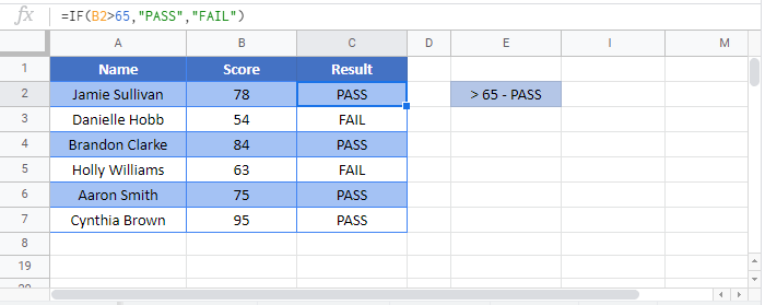
Например, предположим, что вы оцениваете оценки, полученные студентами на экзамене, и хотите знать, сдал ли студент экзамен или нет. В этом случае вы можете использовать функцию IF (ЕСЛИ), и если оценка больше 35, она вернет «Зачёт», иначе вернется «Не зачёт».

IF(logical_expression, value_if_true, value_if_false)

logical_expression — это условие, которое вы проверяете в функции. Это выражение или ссылка на ячейку, содержащую выражение, которое вернет логическое значение, то есть ИСТИНА или ЛОЖЬ.
value_if_true — значение, которое функция возвращает, если логическое_выражение — ИСТИНА.
value_if_false — (необязательный аргумент) значение, возвращаемое функцией, если логическое выражение равно FALSE. Если вы не укажете аргумент value_if_false и проверенное условие не будет выполнено, функция вернет FALSE.

Теперь давайте рассмотрим несколько примеров, чтобы понять, как использовать функцию IF в Google Таблицах в реальных сценариях.

Пример 1: проверка отдельного условия с помощью функции IF

Предположим, у вас есть оценки учащихся на экзамене, и вы хотите указать, сдал ли учащийся или не прошел (как показано ниже).

Вы можете легко узнать это, используя функцию IF в Google Таблицах.

Вот формула, которая сделает это:

=IF(B2>35,"Pass","Fail")

Она проверяет, больше ли баллов 35 или нет. Если это так, то возвращается Pass, иначе возвращается Fail.

Пример 2: проверка нескольких условий с помощью функции IF

Используя тот же пример, что и выше, если у вас есть система оценок в школе, и вы должны выставить оценку ученику на основе полученных оценок.

Например, ученик получает оценку F, если он / она набирает меньше 35, D для оценок от 35 до 50, C для оценок от 50 до 70, B для оценок от 70 до 90 и A выше 90 (как показано ниже ):

В этом случае нужно не только проверить, выше ли отметка 35, но и проверить диапазон, в котором она лежит.

Вот формула, которая даст вам результат в этом случае:

=IF(B2<35,"F",If(B2<50,"D",If(B2<70,"C",If(B2<90,"B","A"))))

Эта формула сначала проверяет, меньше ли результат 35 или нет. Если да, то она возвращает F, иначе переходит к следующему условию и так далее.

Пример 3: Расчет комиссионных с использованием функции IF в Google Таблицах

Функция Google Таблиц If позволяет выполнять вычисления в разделе значений. Хорошим примером этого является расчет комиссии по продажам для торгового представителя с помощью функции IF.

В приведенном ниже примере торговый представитель не получает комиссию, если продажи меньше 50 тысяч, получает комиссию 4%, если продажи составляют от 50 до 80 тысяч, и 10% комиссии, если продажи превышают 80 тысяч.

Вот используемая формула:

=IF(B2<50,0,IF(B2<80,B2*4%,B2*10%))

В формуле, использованной в приведенном выше примере, расчет выполняется внутри самой функции IF. Когда значение продаж находится между 50-100K, возвращается B2 * 4%, что составляет комиссию в размере 4%, основанную на стоимости продажи.

Пример 4: Использование операторов AND/OR в функции IF

В функции IF вы можете использовать операторы AND/OR для одновременной проверки нескольких условий.

Например, предположим, что у вас есть список студентов с их оценками и посещаемостью. Стипендию получают только те студенты, которые набрали более 80 баллов и посещаемость более 80%. Вы можете быстро идентифицировать таких студентов, используя условие AND в функции IF.

Вот формула, по которой будут определены студенты, имеющие право на получение стипендии.

=IF(AND(B2>80,C2>80%),"Yes",”No”)

Она работает, проверяя оба условия в функции AND. Если функция AND возвращает ИСТИНА, функция IF возвращает «Да», иначе она возвращает «Нет».

Источник

Пример использования

Синтаксис

Примечания

Похожие функции

Примеры

Функция IF (ЕСЛИ) в Google таблицах

Примеры функции IF (ЕСЛИ) в Google таблицах

Простой пример функции IF (ЕСЛИ)

Более сложный пример функции IF (ЕСЛИ)

Функция IF (ЕСЛИ) в Google таблицах — несколько условий

Функция IFS (ЕСЛИМН) в Google таблицах

IF Function Overview

How to Use the IF Function

What can IF Return?

Using IF with AND

Using IF with OR

Using IF with XOR

Using IF with NOT

Nested IF Statements

Simplifying Complex IF Statements with Helper Columns

Using Grouping to Hide Helper Columns

The IFS Function

Using IF with Conditional Formatting

Using IF in Array Formulas

IF in Google Sheets

VBA IF Statements

IF Google Sheets function explained

IF Google Sheets syntax

Google Sheets IF formula example

Nested IF Google Sheets statements for multiple logical expressions

Example of a nested IF formula Google Sheets

IF + AND/OR Google Sheets for multiple logical expressions

AND and OR Google Sheets functions explained

IF+AND Google Sheets formula example

IF+OR Google Sheets formula example

IF+AND+OR formula Google Sheets example

IFS Google Sheets function explained

IFS Google Sheets syntax

IFS Google Sheets formula example

IFS vs. multiple IF statements Google Sheets

IFS vs. nested IF statements example

IF, AND, OR, IFS formula examples in real-life use cases

Sales metrics calculated with IF and IFS formulas

Formulas for the Total Deals metric

Formulas for the Revenue metric

Formulas for the Value metric

IFS or nested IF statements in Google Sheets – which are better?

Пример 1: проверка отдельного условия с помощью функции IF

Пример 2: проверка нескольких условий с помощью функции IF

Пример 3: Расчет комиссионных с использованием функции IF в Google Таблицах

Пример 4: Использование операторов AND/OR в функции IF