
If you know the result that you want from a formula, but are not sure what input value the formula needs to get that result, use the Goal Seek feature. For example, suppose that you need to borrow some money. You know how much money you want, how long you want to take to pay off the loan, and how much you can afford to pay each month. You can use Goal Seek to determine what interest rate you will need to secure in order to meet your loan goal.
If you know the result that you want from a formula, but are not sure what input value the formula needs to get that result, use the Goal Seek feature. For example, suppose that you need to borrow some money. You know how much money you want, how long you want to take to pay off the loan, and how much you can afford to pay each month. You can use Goal Seek to determine what interest rate you will need to secure in order to meet your loan goal.
Note: Goal Seek works only with one variable input value. If you want to accept more than one input value; for example, both the loan amount and the monthly payment amount for a loan, you use the Solver add-in. For more information, see Define and solve a problem by using Solver.
Step-by-step with an example
Let’s look at the preceding example, step-by-step.
Because you want to calculate the loan interest rate needed to meet your goal, you use the PMT function. The PMT function calculates a monthly payment amount. In this example, the monthly payment amount is the goal that you seek.
Prepare the worksheet
-
Open a new, blank worksheet.
-
First, add some labels in the first column to make it easier to read the worksheet.
-
In cell A1, type Loan Amount.
-
In cell A2, type Term in Months.
-
In cell A3, type Interest Rate.
-
In cell A4, type Payment.
-
-
Next, add the values that you know.
-
In cell B1, type 100000. This is the amount that you want to borrow.
-
In cell B2, type 180. This is the number of months that you want to pay off the loan.
Note: Although you know the payment amount that you want, you do not enter it as a value, because the payment amount is a result of the formula. Instead, you add the formula to the worksheet and specify the payment value at a later step, when you use Goal Seek.
-
-
Next, add the formula for which you have a goal. For the example, use the PMT function:
-
In cell B4, type =PMT(B3/12,B2,B1). This formula calculates the payment amount. In this example, you want to pay $900 each month. You don’t enter that amount here, because you want to use Goal Seek to determine the interest rate, and Goal Seek requires that you start with a formula.
The formula refers to cells B1 and B2, which contain values that you specified in preceding steps. The formula also refers to cell B3, which is where you will specify that Goal Seek put the interest rate. The formula divides the value in B3 by 12 because you specified a monthly payment, and the PMT function assumes an annual interest rate.
Because there is no value in cell B3, Excel assumes a 0% interest rate and, using the values in the example, returns a payment of $555.56. You can ignore that value for now.
-
Use Goal Seek to determine the interest rate
-
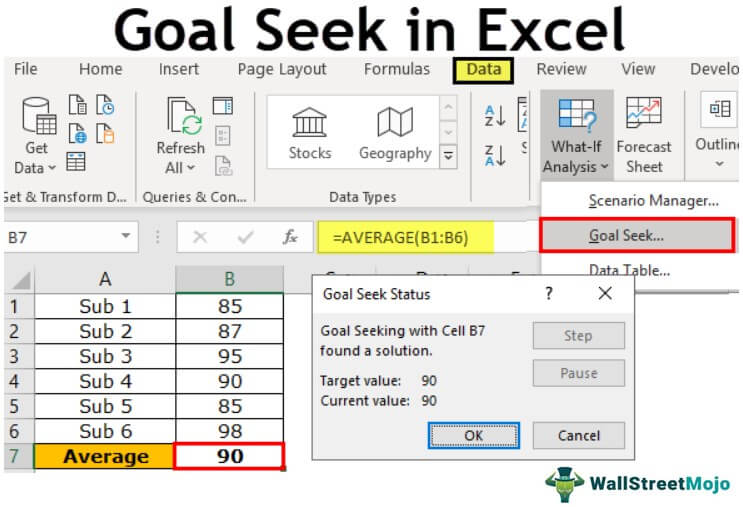
On the Data tab, in the Data Tools group, click What-If Analysis, and then click Goal Seek.
-
In the Set cell box, enter the reference for the cell that contains the formula that you want to resolve. In the example, this reference is cell B4.
-
In the To value box, type the formula result that you want. In the example, this is -900. Note that this number is negative because it represents a payment.
-
In the By changing cell box, enter the reference for the cell that contains the value that you want to adjust. In the example, this reference is cell B3.
Note: The cell that Goal Seek changes must be referenced by the formula in the cell that you specified in the Set cell box.
-
Click OK.
Goal Seek runs and produces a result, as shown in the following illustration.

Cells B1, B2, and B3 are the values for the loan amount, term length, and interest rate.
Cell B4 displays the result of the formula =PMT(B3/12,B2,B1).
-
Finally, format the target cell (B3) so that it displays the result as a percentage.
-
On the Home tab, in the Number group, click Percentage.
-
Click Increase Decimal or Decrease Decimal to set the number of decimal places.
-

If you know the result that you want from a formula, but are not sure what input value the formula needs to get that result, use the Goal Seek feature. For example, suppose that you need to borrow some money. You know how much money you want, how long you want to take to pay off the loan, and how much you can afford to pay each month. You can use Goal Seek to determine what interest rate you will need to secure in order to meet your loan goal.
Note: Goal Seek works only with one variable input value. If you want to accept more than one input value, for example, both the loan amount and the monthly payment amount for a loan, use the Solver add-in. For more information, see Define and solve a problem by using Solver.
Step-by-step with an example
Let’s look at the preceding example, step-by-step.
Because you want to calculate the loan interest rate needed to meet your goal, you use the PMT function. The PMT function calculates a monthly payment amount. In this example, the monthly payment amount is the goal that you seek.
Prepare the worksheet
-
Open a new, blank worksheet.
-
First, add some labels in the first column to make it easier to read the worksheet.
-
In cell A1, type Loan Amount.
-
In cell A2, type Term in Months.
-
In cell A3, type Interest Rate.
-
In cell A4, type Payment.
-
-
Next, add the values that you know.
-
In cell B1, type 100000. This is the amount that you want to borrow.
-
In cell B2, type 180. This is the number of months that you want to pay off the loan.
Note: Although you know the payment amount that you want, you do not enter it as a value, because the payment amount is a result of the formula. Instead, you add the formula to the worksheet and specify the payment value at a later step, when you use Goal Seek.
-
-
Next, add the formula for which you have a goal. For the example, use the PMT function:
-
In cell B4, type =PMT(B3/12,B2,B1). This formula calculates the payment amount. In this example, you want to pay $900 each month. You don’t enter that amount here, because you want to use Goal Seek to determine the interest rate, and Goal Seek requires that you start with a formula.
The formula refers to cells B1 and B2, which contain values that you specified in preceding steps. The formula also refers to cell B3, which is where you will specify that Goal Seek put the interest rate. The formula divides the value in B3 by 12 because you specified a monthly payment, and the PMT function assumes an annual interest rate.
Because there is no value in cell B3, Excel assumes a 0% interest rate and, using the values in the example, returns a payment of $555.56. You can ignore that value for now.
-
Use Goal Seek to determine the interest rate
-
Do one of the following:
In Excel 2016 for Mac: On the Data tab, click What-If Analysis, and then click Goal Seek.
In Excel for Mac 2011: On the Data tab, in the Data Tools group, click What-If Analysis, and then click Goal Seek.
-
In the Set cell box, enter the reference for the cell that contains the formula that you want to resolve. In the example, this reference is cell B4.
-
In the To value box, type the formula result that you want. In the example, this is -900. Note that this number is negative because it represents a payment.
-
In the By changing cell box, enter the reference for the cell that contains the value that you want to adjust. In the example, this reference is cell B3.
Note: The cell that Goal Seek changes must be referenced by the formula in the cell that you specified in the Set cell box.
-
Click OK.
Goal Seek runs and produces a result, as shown in the following illustration.
-
Finally, format the target cell (B3) so that it displays the result as a percentage. Follow one of these steps:
-
In Excel 2016 for Mac: On the Home tab, click Increase Decimal
or Decrease Decimal . -
In Excel for Mac 2011: On the Home tab, under Number group, click Increase Decimal
or Decrease Decimal to set the number of decimal places.
-
 or Decrease Decimal
  .
. or Decrease Decimal
  to set the number of decimal places.
What is Goal Seek in Excel?
The Goal Seek in excel is a “what-if-analysis” tool that calculates the value of the input cell (variable) with respect to the desired outcome. In other words, the tool helps answer the question, “what should be the value of the input in order to attain the given output?”
For example, the cost price of a product is $15 and the business wants to earn revenue of $50,000. The Goal Seek function can determine the number of units of the product to be sold to achieve the given target of $50,000.
The Goal Seek changes the variable (cause) to study the variations in the result (effect). It shows the impact of change in one value on the other value. This is why it is helpful in cause and effect analysis.
Goal seek function in excel is used in financial modeling and forecasting scenarios.
Table of contents
- What is Goal Seek in Excel?
- Goal Seek Parameters
- How to use Goal Seek in Excel?
- Example #1
- Example #2
- Example #3
- The Rules Governing the Parameters
- Frequently Asked Questions
- Recommended Articles
Goal Seek Parameters
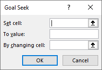
The parameters to be specified in the “Goal Seek” dialog box are stated as follows:
- Set cell–In this box, enter the cell reference of the formula to be resolved. This is the target cell or the formula cell.
- To value–In this box, enter the desired output to be achieved. This is the value of the “set cell” to be attained.
- By changing cell–In this box, enter the reference of the input cell (variable) to be adjusted. This is the cell we want to change in order to impact the “set cell.”
Note: At a given time, Goal Seek works with only one variable input. For working with multiple input values, use the solver in Excel.
How to use Goal Seek in Excel?
Example #1
You can download this Goal Seek Excel Template here – Goal Seek Excel Template
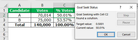
The following table shows the votes received by the two candidates, A and B, who contested in an election. In the present situation, candidate B is leading by 10,000 votes. It is given that to win the election, 50.01% votes are required.
We want to change the voting percentage (column C) of candidate A in such a way that he wins the election. Calculate the total number of votes required by candidate A to win.

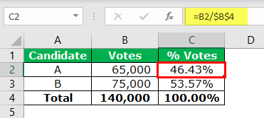
Let us calculate the present voting percentage for both the candidates. This is done by dividing the individual votes received by the total votes.
Candidate A has won 46.43% of the total votes. Therefore, he needs only 3.67% votes to win the election.
The steps to use Goal Seek in excel are stated as follows:
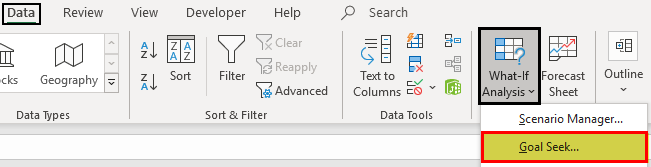
- In the Data tab, click “Goal Seek” from the “what-if-analysis” drop-down.

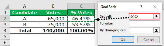
- The “Goal Seek” excel window appears as shown in the following image.

- Enter $C$2 in the “set cell” box. This is because C2 is the target cell.

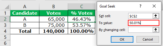
- Enter 50.01% in the “to value” box. This is the value of the “set cell” that we want to obtain. In other words, the “set cell” should change to the target value of 50.01%.

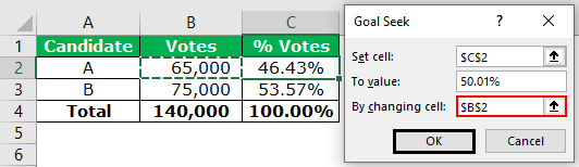
- Enter $B$2 in the “by changing cell” box. This is the cell we want to change to impact the “set cell” C2. Since all the parameters are set, click “Ok” to get the result.

- The output is shown in the following image. Candidate A should secure 70,014 votes to win the election. With 70,014 votes, the voting percentage of candidate A will become 50.01%. Click “Ok” to apply the changes.

The total number of votes and the voting percentage of candidate A has changed. Consequently, the votes and the voting percentage of candidate B also changes.
The votes of candidate B are calculated by subtracting 70,014 from 140,000. The final output is displayed in the following image. Hence, candidate A wins the election.


Example #2
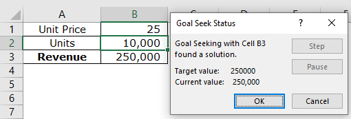
Mr. A opens a retail shop and sells goods at an average selling price of $25 per unit. To meet his operating expenses, he wants to generate monthly revenue of $250,000.
We want to calculate the quantity of the goods Mr. A should sell to earn the given revenue.
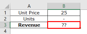
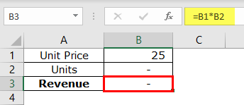
Step 1: In cell B3, apply the formula unit priceUnit Price is a measurement used for indicating the price of particular goods or services to be exchanged with customers or consumers for money. It includes fixed costs, variable costs, overheads, direct labour, and a profit margin for the organization.read more*units (B1*B2).
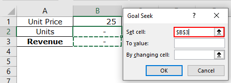
Step 2: In the Data tab, click “Goal Seek” from the “what-if-analysis” drop-down. The “Goal Seek” window appears as shown in the following image.
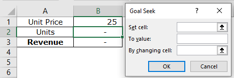
Step 3: Enter $B$3 in the “set cell” box. The target cell is the revenue cell B3.
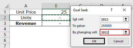
Step 4: Enter 250000 in the “to value” box. This is the value of the “set cell” to be achieved.

Step 5: Enter $B$2 in the “by changing cell.” The quantity has to be calculated in cell B2. So, this is the cell that has to be adjusted to achieve the given revenue. Click “Ok.”
Step 6: The output is displayed in the following image. Hence, Mr. A needs to sell 10,000 units of goods to generate revenue of $250,000. Click “Ok” to apply the changes.
Example #3
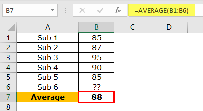
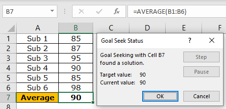
The following table shows the marks obtained (in percentage) by a student in five subjects. Her present average grade is 88%. Since there are six subjects in the class, she is yet to appear for the last examination.
The student is targeting the overall average of 90% from all the six subjects. We want to calculate the marks she should score in the remaining subject to secure the given average.
Step 1: Open the “Goal Seek” window from the Data tab.
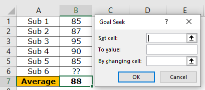
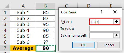
Step 2: Enter $B$7 as the “set cell.” The target cell is the average cell B7.
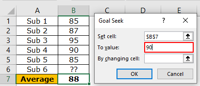
Step 3: Enter “90” in the “to value” box. This is the value we want to attain.
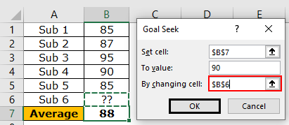
Step 4: Enter $B$6 in the “by changing cell” box. This is the value that has to be adjusted. Click “Ok.”
Step 5: The output is displayed in the following image. Hence, the student should score 98% in “subject 6” to get an overall average of 90%. Click “Ok” to apply the changes.
Likewise, the Goal Seek helps identify the exact input that should be adjusted to reach the desired result.
The Rules Governing the Parameters
- The “set cell” should always contain a formula.
- The formula of the “set cell” should depend, whether directly or indirectly, on the “by changing cell.” This is necessary to study the impact on the “set cell.”
- The “by changing cell” should not contain any special characters.
Frequently Asked Questions
Define the Goal Seek in Excel.
The Goal Seek in excel calculates the input value (variable) based on a given output. Being a what-if-analysis tool, the Goal Seek is used when there is a need to study the impact of a change in one value on the other.
The Goal Seek is used in scenario analysis, cause and effect situations, break-even model, sensitivity analysis, and so on. The parameters used in the Goal Seek excel tool are listed as follows:
• “Set cell”–This is the reference of the formula cell.
• “To value” –This is the desired or targeted value to be achieved.
• “By changing cell” –This is the cell reference of the variable to be changed for attaining the desired value.
The Goal Seek works with one input at a given time.
What is Goal Seek used for in Excel?
The Goal Seek in excel is used in the following situations:
• To calculate the input (unknown) for a given output (known)
• To analyze the impact of a change in the input (variable) on the output (set cell)
• To perform what-if-analysis, i.e., explore the various outcomes if different values are used for the input
• To return the closest value (approximate) in case a solution to the problem is not found
Note: The formula used in the Goal Seek analysis remains the same throughout. The input values entered in the “by changing cell” box are changed to study the effect on the output.
How does the Goal Seek work in Excel?
The Goal Seek does backward calculations. It begins from the output that is known and returns the exact input. This input is a requisite for reaching the given output.
The steps showing the working of Goal Seek are listed as follows:
1. Enter data in Excel on which calculations using Goal Seek are to be performed.
2. Click “Goal Seek” from the “what-if-analysis” drop-down in the Data tab.
3. Enter the parameters in the tool.
a. Type the cell reference for the input and the output.
b. Type the target value to be achieved.
4. Click “Ok” to proceed.
5. In the “Goal Seek status” box, click “Ok” to apply the changes to the worksheet.
Note: The initial values can be restored by pressing the “undo” shortcut (Ctrl+Z).
Recommended Articles
This has been a guide to Goal Seek in Excel. Here we learn how to use Goal Seek function in Excel along with step by step examples and a downloadable template. You may learn more about Excel from the following articles –
- Evaluate Formula in ExcelThe Evaluate formula in Excel is used to analyze and understand any fundamental Excel formula such as SUM, COUNT, COUNTA, and AVERAGE. For this, you may use the F9 key to break down the formula and evaluate it step by step, or you may use the “Evaluate” tool.read more
- Create a Data Table in ExcelA data table in excel is a type of what-if analysis tool that allows you to compare variables and see how they impact the result and overall data. It can be found under the data tab in the what-if analysis section.read more
- One Variable Excel Data TableOne variable data table in excel means changing one variable with multiple options and getting the results for multiple scenarios. The data inputs in one variable data table are either in a single column or across a row.read more
- Excel Scenario ManagerScenario Manager is a what-if analysis tool that works with many scenarios that are supplied to it. It uses a set of ranges that have an effect on a certain output and can be used to generate different scenarios such as bad and medium depending on the values.read more
- Excel Shortcut Paste ValuesPasting values is a common procedure that allows us to eliminate any formatting and formulas from the copied cell and paste them into the pasted cell. «Alt + E + S + V» is the shortcut key for pasting values.read more
 One of the most popular group of features in Excel are the What-If Analysis tools. In Microsoft’s words, What-If Analysis tools allow you to “try out various values for the formulas in your sheet“.
This particular Excel tutorial focuses on 1 of these What-If Analysis tools: Goal Seek.

Learning how to use Goal Seek is extremely helpful because, as I explain below, you can use Goal Seek whenever you know the resulting value that you want a particular formula to return but aren’t sure what is the precise input that is required to achieve that result.
My purpose with this Excel tutorial is to provide all the information you need to start using Goal Seek now. Therefore, in addition to introducing and explaining how you can use Goal Seek, I show how you can deal with some common challenges you may face when working with this feature.
Additionally, since one of my main focuses at Power Spreadsheets is Visual Basic for Applications, the second part of this blog post explains how you can use Goal Seek (and deal with some of the challenges arising in connection with it) with VBA.
As with all other Excel and VBA tutorials in Power Spreadsheets, this blog posts includes a detailed practical example that shows (step-by-step) how to implement everything.
You can use the following table of contents to navigate to the section that interests you the most:
Before we dive into Goal Seek, let’s start by taking a look at the…
Example For This Tutorial
This Excel VBA Goal Seek Tutorial is accompanied by an Excel workbook containing the data and macros I use in the examples below. You can get immediate free access to this example workbook by subscribing to the Power Spreadsheets Newsletter.
In this particular example, we’ll be taking a look at the exam scores obtained by a certain University student named Lisa Stephens.
Let’s assume that, on this semester, Lisa Stephens is taking a class that is graded through 3 exams. Each of the exams has exactly the same weight. Therefore, her final score is determined by averaging her scores in those 3 exams.
In order to use Excel to determine Lisa’s final score, you can set up a formula that uses the AVERAGE function. Such a formula calculates Lisa’s final score automatically once you enter her individual scores in each of the 3 exams.

Let’s assume that Lisa Stephens has already taken 2 out of the 3 exams. Her scores in these 2 exams where 77.0% and 57.0%.

Now, let’s assume that you want to carry out some scenario analysis.
One approach you can take is to enter different scores for Exam 3. Excel automatically calculates Lisa’s Final score. For example, if I enter 87.0%, Excel determines that Lisa’s Final score is 73.7%.

In such a case, the question you’re asking to Excel is: what is Lisa Stephens’ Final score if her score in Exam 3 is 87.0%?
Now, let’s assume further that Lisa Stephens needs to achieve a Final score of at least 75.0%. In such a situation, you may be interested in knowing what is the minimum score Lisa must get in Exam 3 for purposes of achieving a Final score of 75.0%.
Theoretically, you can continue with the same approach. You can plug different values in cell E6 (the score for Exam 3) until, eventually, you plug in the score that results in Lisa’s Final score being 75.0%.
This may not be the most efficient way to proceed.
What I mean is that, in such situations, you may want to take the opposite approach. This means that you may want to ask Excel a different question. Instead of asking what is Lisa’s Final score if her score in Exam 3 is #, you can ask: what is the score that Lisa Stephens must achieve in Exam 3 in order to get a Final score of 75.0%?
In the following sections, I explain how you can answer this question, and those that have a similar structure, by using the Range.GoalSeek VBA method.
Let’s start by taking a look at…
As explained at office.com:
If you know the result you want from a formula, but you aren’t sure which input value the formula needs to get that result, use the Goal Seek feature.
In other words, you can use the Excel Goal Seek tool for purposes of determining the value that you must enter in a particular cell (the Changing Cell) to get the result you want (the Goal) in another cell that depends on the Changing Cell. To a certain extent, Goal Seek is the (rough) opposite of worksheet formulas.
Goal Seek uses a single variable input value. This means that there’s only one Changing Cell.
If you’re working with more than one input (Changing) cell, the appropriate tool is usually Solver. I may cover Solver in a future tutorial. If you want to be notified by email every time that I publish new content in Power Spreadsheets, please register for our newsletter by entering your email address below.
In the words of Excel guru John Walkenbach (in the Excel 2016 Bible):
Single-cell goal seeking is a rather simple concept.
Therefore, let’s go back to the practical example I introduce above. The question we want Excel to help us answer is as follows:
What is the score that Lisa Stephens must achieve in Exam 3 in order to get a Final score of 75.0%?
At this point, the relevant table in the Excel worksheet we’re working with looks as follows:

And the question you’re asking looks something like this:

You can get Excel to provide you the value that should go in cell E6 (score in Exam 3) so that the value in cell F6 (Final score) is equal to 75.0% by following these 3 easy steps:
Step #1: Display The Goal Seek Dialog Box
To open the Goal Seek dialog box, proceed as follows:
- Step #1: Go to the Data tab of the Ribbon.
- Step #2: Click on “What-If Analysis”.
- Step #3: Once Excel displays the drop-down, click on “Goal Seek…”.

Alternatively, you can use the keyboard shortcuts “Alt + A + W + G” or “Alt + T + G”.
Once you’ve completed the 3 steps above (or entered the keyboard shortcut) Excel displays the Goal Seek dialog box.

Step #2: Provide The Relevant Information In The Goal Seek Dialog Box
As you can see in the dialog box above, the Goal Seek dialog box asks you for the following 3 inputs:
- Input #1: Set cell.
This is the dependent cell that holds the formula for which you want to seek a Goal. In this input field, you must specify a reference to a single cell that holds a formula.

- Input #2: To value.
This is the value that you want the formula in the dependent cell (which you specify in input #1 above) to return. In this input field, you must enter a hard-coded value.
- Input #3: By changing cell.
This is the Changing Cell. In other words, this is the cell whose value Excel must adjust so that the formula in the dependent cell (specified in input #1) returns the value you want (specified in input #2 above).


In the example we’re looking at, the relevant inputs are as follows:
- Input #1 (Set cell) is a reference to cell F6. This cell holds the formula that uses the AVERAGE function to calculate Lisa Stephens’ Final score.
- Input #2 (To value) is the value 75%. This is the Final score that Lisa must achieve, as explained above.
- Input #3 (By changing cell) is a reference to cell E6. This is the cell where the Exam 3 score goes.

Once you’ve provided the relevant input in the Goal Seek dialog box, you can click the OK button on the lower section of the dialog box.

Step #3: Replace Value In Changing Cell Or Restore It
After you’ve completed step #2 above, Excel displays the Goal Seek Status dialog box.
Excel uses this dialog box to inform you about the following details:
- #1: Whether Excel has been able (or not) to find a solution.
- #2: What is the target value that you entered in the Goal Seek dialog box (input #2 in the previous step #2).
- #3: What is the current value of the dependent cell for which you’re seeking a Goal (input #1 in the previous step #2).
In the example we’re using in this tutorial, this dialog box looks as follows once the goal seeking process is completed. Notice the 3 pieces of data I mention above:

Excel also displays the results it has found in the worksheet. Notice how, in the following screenshot, Excel shows that Lisa Stephens must achieve a score of 91.0% in the third exam in order to have a Final score of 75.0%.

At this point, you can click on either of 2 buttons at the bottom of the dialog box:

- OK: If you click on OK, Excel replaces the value in the Changing Cell (input #3 in step #2 above) with the value it has found through the Goal Seek process.
As I mention above, in the example we’re looking at, Excel sets the value for the Exam 3 score to be 91.0%. This is the minimum score that Lisa Stephens must achieve in order to obtain a Final score of at least 75.0%.

- Cancel: If you click the Cancel button, Excel restores the worksheet to the same state it had before you launched the Goal Seek dialog box in step #1 above.


Before we jump onto the section where I explain how you can do all of the above by using Visual Basic for Applications, let’s take a look at some…
Common Goal Seek Problems
The following are some common problems or challenges that you may encounter from time-to-time when using the Excel Goal Seek tool:
Problem #1: Goal Seek May Not Have Found A Solution
In some situations, the Goal Seek Status dialog box may inform you that Goal Seeking “may not have found a solution”.

In such situations, the value that Goal Seek sets for the Changing Cell (E6 in the screenshot above) doesn’t (usually) make sense.

Broadly speaking, you can usually classify the reasons why this happens in the following 2 groups:
Reason #1: There Is No Solution To The Goal Seek Problem
As a general rule, the cells that you specify in both (i) the Set cell and (ii) the By changing cell input fields must have a precedent-dependent relationship. More precisely, the cell you specify in the Set cell input field must be a dependent of the Changing Cell.

Excel worksheets can be very complex. In certain circumstances, it may be difficult to ensure that there’s a dependent-precedent relationship between the 2 cells that you specify in the Goal Seek dialog box.
Therefore, if Excel tells you that Goal Seeking may not have found a solution, one of the first things you should check is the logic of the worksheet. In other words, make sure that
- #1: There is a precedent-dependent relationship between the cells that you specify as input in the Goal Seek dialog box.
- #2: The Goal Seek problem actually has a solution.
Despite the above, there are situations where there’s a solution but Excel seems to be unable to find it. These cases may fall under…
Reason #2: Excel Isn’t Carrying Out Enough Iterations To Find A Solution
When you use the Goal Seek tool, Excel follows an iterative process for purposes of finding a solution. As explained by Excel authority Bill Jelen (Mr. Excel) in Excel 2016 in Depth, this basically means that Excel plugs in different values in the Changing Cell until it finds a value that solves the problem.
The following GIF shows how the Goal Seek Status dialog box looks like while Excel carries out the Goal Seeking process for this tutorial’s example. I’ve adjusted the playback speed to create the slow motion effect and make the process easier to see. Notice how the contents of the Goal Seek Status dialog box change as the process advances:

Excel has a particular setting that sets the maximum number of iterations that it makes when an iterative calculation is undertaken. This maximum number of iterations applies to the Goal Seek tool.
Therefore, if Excel doesn’t find a solution after undertaking that maximum number of iterations, it stops trying. In such cases, the Goal Seek Status dialog box informs you that Goal Seeking may not have found a solution.

In most situations, you can usually handle this challenge by implementing 1 or both of the following solutions:
Solution #1: Enter A Value In The Changing Cell That Is Closer To The Solution.
You might think this suggestion is crazy.
After all, you want Excel to tell you what is the value that should go in the Changing Cell. So:
Why would I suggest entering a value in that cell?
The logic behind this suggestion is that, if you enter a value that is closer to the solution in the Changing Cell, the number of iterations that Excel must undertake before finding a solution usually decreases. This is the case because Excel uses the current value in the Changing Cell as the base from which the iterative process begins.
Therefore, as a general rule:
The farther away the current value in the Changing Cell is from the solution, the higher the number of iterations needed to find a solution.
To see how this works in practice, let’s go back to Lisa Stephens’ test scores. Compare the following 2 GIFs and notice the difference in speed and number of iterations required. In order to make the whole process easier to follow, I’ve adjusted the motion speed of both GIFs.
- GIF #1: In this case, I leave cell E6 (Exam 3 score) empty.

- GIF #2: In this case, I set the initial value of cell E6 to be equal to 70.0% prior to carrying out the Goal Seek.


Solution #2: Increase The Maximum Number Of Iterations That Excel Undertakes.
If you implement it properly, solution #1 reduces the number of iterations that Excel requires to find a solution.
This solution #2 attacks the problem from a different perspective. It increases the number of iterations carried out by Excel before it “gives-up” and tells you that Goal Seeking may not have found a solution.
You can increase the maximum number of iterations that Excel undertakes in the following 4 easy steps:
- Step #1: Click on the File tab of the Ribbon.

- Step #2: Once you complete step #1, Excel takes you to the Backstage View. Here, click on “Options” on the lower section of the sidebar that appears on the left side of the screen.

- Step #3: Once you’ve completed the previous steps, Excel displays the Excel Options dialog. Within the Excel Options dialog box, select the Formulas tab on the left sidebar.

- Step #4: Change the maximum number of iterations by setting the value of the Maximum Iterations input field and click the OK button on the lower right corner of the Excel Options dialog box to confirm the changes.


If you’re like me and prefer using keyboard shortcuts, you can replace the steps above by the following 3 simple steps:
- Step #1: Use the keyboard shortcuts “Alt + T + O + F + (Alt + X)” or “Alt + F + T + F + (Alt + X)”. These keyboard shortcuts take you directly to the input field for Maximum Iterations.
- Step #2: Enter the new value for Maximum Iterations.
- Step #3: Press the Enter key to confirm your choice,
Problem #2: Goal Seek Isn’t Precise Enough
As explained in the Excel 2016 Bible:
Like all computer programs, Excel has limited precision.
In some circumstances, you may find that Excel returns a solution that is too far from the value that you’re expecting (or looking for).
The cause of this is, usually, related to the iterative process used by Goal Seek. The reason for this is that, in addition to having a setting for the maximum number of iterations that Excel undertakes (which I explain above), Excel also has a setting that controls the maximum change between iterations. This setting also applies to the Goal Seek tool.
The Maximum Change between iterations setting determines when Excel considers that Goal Seeking has found a solution. More precisely, once the difference between (i) the current value of the dependent cell you’re working with (specified in the Set cell input field of the Goal Seek dialog) and (ii) the target value (specified in the To value input field of the Goal Seek dialog) is smaller than the Maximum Change between iterations, Excel considers that it has found a solution.
Mathematically, Excel considers it has found a solution when the following condition is met:
| Set cell – To value | < Maximum Change between iterations
Once this condition is met, the Goal Seek tool provides you with the current value as a solution to the problem you’ve set up.
Assuming that you don’t want to change the input you’ve provided in the Set cell and To value input fields of the Goal Seek value, the item you must focus on is the Maximum Change between iterations.
More precisely, you’ll want to make the Maximum Change between iterations smaller. This forces the Goal Seek feature to provide a more accurate solution.
You can decrease the Maximum Change between iterations by following 4 simple steps:
- Step #1: Click on the File tab.

- Step #2: Click on “Options” on the lower left side of the Backstage.

- Step #3: Select the Formulas tab within the Excel Options dialog box.
- Step #4: Change (decrease) the value for Maximum Change and click on the OK button on the lower right corner of the dialog.


If you want to use keyboard shortcuts, you can change the Maximum Change between iterations in the following 3 easy steps:
- Step #1: Use the keyboard shortcuts “Alt + T + O + F + (Alt + C)” or “Alt + F + T + F + (Alt + C)” to get to the Maximum Change input field in the Excel Options dialog.
- Step #2: Enter a new value for Maximum Change.
- Step #3: Press the Enter key.
Problem #3: The Goal Seeking Problem Has Multiple Solutions
Some Goal Seek problems may have (theoretically) multiple solutions.
In the Excel 2016 Bible, John Walkenbach provides a typical example of such situation: problems involving square numbers or square roots. The reason why such problems may have multiple solutions is because any positive real number has 2 square roots. One of these square roots is positive and the other is negative.
When facing such situations, you may want to refer to my explanation above regarding how the iterative process used by the Goal Seek tool works. Of particular importance is the fact that Excel uses the current value of the Changing Cell as the base from which the iterations begin.
The consequence of this, as explained by John Walkenbach in the Excel 2016 Bible, is that:
If you use goal seeking when multiple solutions are possible, Excel gives you the solution that is closest to the current value.
Therefore, in such cases, you may want enter a value in the Changing Cell input field that is closer to the solution.
Problem #4: Goal Seek Slows Down Excel
Each Goal Seek iteration triggers the recalculation of all open workbooks.
This is something you may want to consider as you structure the Excel workbooks you use Goal Seek on. Generally, it’s preferable to have a single workbook (fast and small) open whenever you’re using the Goal Seeking tool.
Theoretically, you may be able to partially address this problem by adjusting Excel’s iteration settings. However, before modifying these settings, bear in mind the following:
- Reducing the maximum number of iterations that Excel can make may result in Excel not being able to find a solution, as I explain above.
- Increasing the maximum change between each iteration may result in Excel returning inaccurate or imprecise values, as I show above.
After reading the previous sections, you probably have a very good grasp of Excel’s Goal Seek feature. The following sections show how you can use Visual Basic for Applications to work with Goal Seek and specify several of the settings that I mention above.
Let’s start by taking a look at the most basic VBA construct you’ll be working with, the…
Range.GoalSeek Method
The main purpose of the Range.GoalSeek method is to calculate the value that is necessary to achieve a particular goal. You generally use the GoalSeek method to calculate the value that, when supplied to a particular formula, “causes the formula to return the number you want”.
The basic syntax of the Range.GoalSeek method is as follows:
expression.GoalSeek(Goal, ChangingCell)
The following are the main items of this syntax:
- expression: Placeholder for a Range object. When you’re working with the GoalSeek method, this Range object must be composed of a single cell.
- Goal: The value that you want Excel to return in the cell that you identify within the expression item above.
In other words, Goal is (as implied by its name) the goal you’re trying to achieve.
- ChangingCell: The (single) cell that Excel must change in order to achieve the Goal.
Range.GoalSeek Method Macro Example
Let’s go back to the sample Goal Seek problem that I introduce and solve manually above.
The following image shows the data we’re working with. As a reminder, our purpose is to find what is the score that Lisa Stephens must get in Exam 3 in order to achieve a Final score (average of the scores in the 3 exams) of 75.0%.

The following simple macro (Goal_Seek_Sample) uses Goal Seek to find this value:

This particular VBA Sub procedure is very simple. However, in order to make everything extremely clear, let’s take a look at each line of code.
Note that, strictly speaking, the macro has a single statement. I divide it in 3 separate lines using the line-continuation character ( _) to improve readability.
Line #1: Range(“F6”).GoalSeek
This line of VBA code calls the Range.GoalSeek method. In particular, notice how this line follows the basic syntax of the GoalSeek method that I explain above.
In this example, the Range object the GoalSeek method works with is cell F6 (Range(“F6”)) of the active worksheet. The single-cell Range object that you specify here is the one that, when using Goal Seek manually, goes in the Set cell input field of the Goal Seek dialog.

As I explain here, this simplified object reference (Range(“F6”)) assumes that you’re working with (i) the Application object, (ii) the active workbook, and (iii) the active worksheet.
Line #2: Goal:=0.75
This line sets the value of the Goal parameter of the GoalSeek method.
In the example we’re working with, this value is equal to 0.75 (75.0%).
The value that you set for this argument is the value you enter in the To value input field of the Goal Seek dialog (if carrying out the Goal Seek manually).

Line #3: ChangingCell:=Range(“E6”)
This line sets the ChangingCell parameter of the Range.GoalSeek method.
In the example we’re looking at, the specified one-cell Range object is cell E6 of the active worksheet.
This argument is the equivalent of the one you enter in the By changing cell input field of the Goal Seek dialog.

The following screenshot shows the results I obtain when executing the sample Goal_Seek_Sample macro on the data within the workbook that accompanies this tutorial.

Notice that the results are exactly the same as those obtained manually above. In other words, the sample Goal_Seek_Sample Sub procedure achieves the same goal.
Now that you have seen how to use the GoalSeek method in Excel, let’s take a look at…
How To Modify Iteration Settings With VBA: Application.MaxIterations And Application.MaxChange Properties
In the section about common Goal Seek problems above, I provide some examples of challenges that you may encounter when using Goal Seek. As I explain then, there are 2 Excel settings that determine how Excel carries out the iterative goal seeking process:
- Maximum Iterations.
- Maximum Change.
You can also manipulate both of these settings with Visual Basic for Applications. Therefore, let’s take a look at the relevant VBA properties:
Application.MaxIterations Property
The Application.MaxIterations property is a read/write property. Its main purpose is as follows:
- If you’re reading the property, it returns the maximum number of iterations that Excel can use.
- If you’re setting the property, you use it to set the maximum number of iterations that Excel can use.
The basic syntax of MaxIterations is as follows:
expression.MaxIterations
“expression”, within the above syntax, is a variable representing an Application object.
Application.MaxChange Property
Just as the Application.MaxIterations property, the Application.MaxChange property is read/write. Its main purpose is as follows:
- If you’re fetching the property’s value, it returns the maximum amount of change between iterations.
- If you’re writing the property, it sets the maximum amount of change between each iteration.
The basic syntax of the MaxChange property is substantially the same as that of MaxIterations. More precisely, the syntax of Application.MaxChange is:
expression.MaxChange
For these purposes, “expression” is a variable representing an Application object.
The sample Goal Seek problem that I use throughout this Excel tutorial is relatively simple. Therefore, I don’t encounter any of the challenges that sometimes arise due to Excel’s iteration settings.
However, to the extent that you may eventually have to deal with such situations, let’s take a look at a practical VBA code example to modify such settings:
Sample VBA Code To Modify Iteration Settings
The following sample macro (Goal_Seek_Iteration_Sample) adjusts Excel’s iteration settings prior to solving the sample Goal Seek problem that we’ve looked at throughout this blog post:

Notice that the second part of the Sub procedure is simply the statement that I explain above. This statement uses the Range.GoalSeek method to solve the sample problem.

Since I explain these 3 lines of code in a previous section, lets focus only on the first 4 lines of VBA code. These are the ones that deal with Excel’s iteration settings.
Lines #1 And #4: With Application | End With
These 2 lines open and close (respectively) a With… End With block.
The effect of using the With statement is that the series of statements within the block (lines #2 and #3 below) are executed on a single object. The single object is specified in the opening statement. In this case, that object is the Application object.
In other words, the effect of the With… End With block is that lines #2 and #3 below work on the Microsoft Excel application (the Application object).
Line #2: .MaxIterations = 100
This line of code uses the Application.MaxIterations property to set the maximum number of iterations that Excel can use to be 100. You can, obviously, use a different value depending on your purposes.
I explain how to modify this setting manually above. As shown there, using the Application.MaxIterations property is the equivalent of setting the value of Maximum Iterations within the Formulas tab of the Excel Options dialog box.

Line #3: .MaxChange = 0.001
Similar to line #2, this line of code sets an iteration-related property. In this case, the Application.MaxChange property is used to set the maximum amount of change between each iteration to be 0.001. You can set a different value if required to achieve your goals.
Using the Application.MaxChange property for these purposes is the equivalent of setting the Maximum Change value within the Formulas tab of the Excel Options dialog. I explain how to do this manually in a previous section of this Excel tutorial.

As you’d expect, executing the Goal_Seek_Iteration_Sample macro on the workbook that accompanies this tutorial achieves exactly the same result as that obtained when executing the Goal_Seek_Sample example macro above.

However, by using the sample VBA code that I provide above, you should be able to easily adjust Excel’s iteration settings in other situations where you’re dealing with more complex Goal Seeking problems.
Conclusion
After reading this Excel tutorial on Goal Seek, you probably have a very good idea of how the Goal Seek tool can help you achieve your goals. More precisely, you’ve read about:
- What is Goal Seek.
- How to use Goal Seek, both manually and with Visual Basic for Applications.
- What are some of the most common problems and challenges that you may encounter while using Goal Seek.
- How you can deal with these challenges, both manually and using VBA.
This Excel VBA Goal Seek Tutorial is accompanied by an Excel workbook containing the data and macros I use in the examples above. You can get immediate free access to this example workbook by subscribing to the Power Spreadsheets Newsletter.
Books Referenced In This Excel Tutorial
- Jelen, Bill (2015). Excel 2016 in Depth. United States of America: Pearson Education Inc.
- Walkenbach, John (2015). Excel 2016 Bible. Indianapolis, IN: John Wiley & Sons Inc.
Have you ever stared at your spreadsheet and wondered how to find the answer to a “what-if” scenario? Let’s start with the goal in mind. In this tutorial, you’ll learn how to use Goal Seek in Excel to answer these and other analysis questions. (Includes video and example spreadsheet.)
What is Goal Seek in Excel?
Goal seek is a built-in function in Microsoft Excel that allows you to see which data item in a formula affects another. You might look at these as “cause and effect” scenarios. It’s sometimes called sensitivity analysis. The “what-if” analysis tool is often used in finance or sales scenarios, such as determining a monthly payment or bonus calculations. There are other uses for it, too.
For example, you might be looking at your local election results and see:
| Decision | Votes | % of Votes |
|---|---|---|
| YES | 4478 | 63.90 * |
| NO | 2530 | 36.10 |
| Total | 7008 | 100 |
* Needs approval from 2/3 of the voters
In our example, the YES votes are a majority but shy of the required 2/3 approval to win the election. People quickly realize they were close, but which item do they change to find out how close. What would’ve made a difference?
Using Goal Seek, we can change the input value of one cell and see how the results change. This would allow you to answer these types of questions.
- How many more YES votes were needed to win the election?
- If 500 more people voted, could the YES voters have won?
The goal of each of these questions is to change one data value to see if the YES percentage went over that two-thirds mark, or 67%. Then, rather than haphazardly changing original values to see the results, Goal Seek can find the answer. It works in the background doing iterative calculations.
While you might think this feature can be used with the Excel formula bar, it can’t. There is no such thing as an Excel Goal Seek formula. Instead, there is a dedicated dialog box with defined fields.
Keyboard Shortcut: Alt + D + W + G
Time needed: 5 minutes.
This tutorial will show you how to invoke the Goal Seek dialog box and fill in the values for your “what-if” scenario. In this example, I will change the YES%.
- Create an Excel spreadsheet with your data or download the practice worksheet.
In the snapshot below, the green cells have formulas to calculate the percentage and totals.

- Click the cell you want to change.
This cell is called the “Set Cell“. In my example, it will be cell D4.
- From the Data tab, select the What if Analysis… button.
- Select Goal Seek from the drop-down menu.
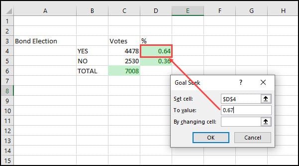
- In the Goal Seek dialog box, enter the new “what if” amount in the To value: field.
In this example, we’re asking Excel to replace the contents of cell D4, which is 0.64, with 0.67. This is the percentage needed to win the election.
- Click the cell you wish to change. Since we wanted to know the number of “Yes” votes needed, we’ll click cell C4. This is our input cell.
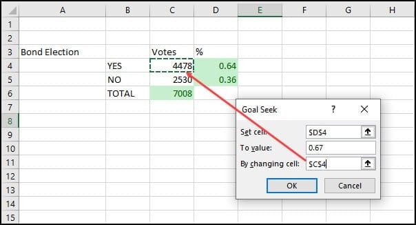
- Click the OK button. Excel will overwrite the previous cell value with the new one.

- If you wish to accept the new value, click OK. Otherwise, click Cancel.
Goal Seek Requirements
As with many simple tools, there are limitations. To start, the tool only works on desktop versions, so if you’re using the web version or on an Ipad, you’re out of luck.
Excel also requires that the Set cell be a formula cell. In my case, I have =C4/C6 to get a percent.
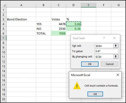
Excel only allows you to change one variable input. The other requirement is that the cell you change in Step 6 (By changing cell:) can’t contain a formula. Instead, it must be a typed value.
Approximation Issues & Formulas
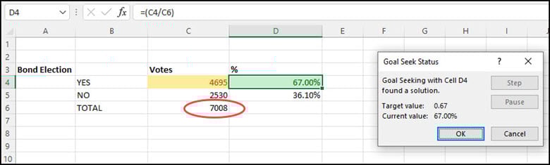
This tool is fine for many scenarios, but it presents a problem here. If you look at the latest figures, you’ll see it also increased the TOTAL vote count. Ideally, I would want to add a constraint and not have my TOTAL vote count go over the current count.
You may have noticed, that I ran into the approximation issue. Goal Seek rounded down my percentage to below 67%.
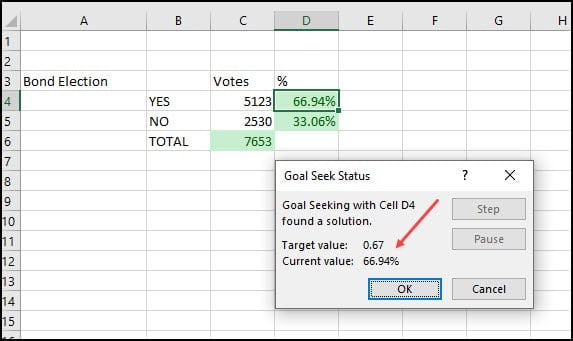
Just as I used a formula in my set cell, I also used an Excel formula cell for TOTAL in B6. This was the SUM of my YES and NO votes. Since this TOTAL cell was a formula, my TOTAL count automatically adjusted when Goal Seek changed the YES cell value.
The solution is to remove my formula and type “7008” in cell C6. This is a more desirable outcome.
While it doesn’t happen often, the tool can sometimes present puzzling results. I’ve seen reports, where some Add-on, has interfered in the calculation. If that happens to you, I would close Excel and open it in Safe Mode.
As this example shows, Goal Seek is a useful “What if” analysis tool that quickly finds the answers for different scenarios. If you’re working with complicated spreadsheets containing many different variables and formulas, then using an add-on called the Excel Solver may be a better solution. However, Goal Seek is a fast solution to lots of scenarios with items such as annual interest rates or sales goals.
Excel Goal Seek Video
Please click the image below to be taken to the video tutorial page and transcription.

Goal Seek Example Spreadsheet

Очень полезной функцией в программе Microsoft Excel является Подбор параметра. Но, далеко не каждый пользователь знает о возможностях данного инструмента. С его помощью, можно подобрать исходное значение, отталкиваясь от конечного результата, которого нужно достичь. Давайте выясним, как можно использовать функцию подбора параметра в Microsoft Excel.
Суть функции
Если упрощенно говорить о сути функции Подбор параметра, то она заключается в том, что пользователь, может вычислить необходимые исходные данные для достижения конкретного результата. Эта функция похожа на инструмент Поиск решения, но является более упрощенным вариантом. Её можно использовать только в одиночных формулах, то есть для вычисления в каждой отдельной ячейке нужно запускать всякий раз данный инструмент заново. Кроме того, функция подбора параметра может оперировать только одним вводным, и одним искомым значением, что говорит о ней, как об инструменте с ограниченным функционалом.
Применение функции на практике
Для того, чтобы понять, как работает данная функция, лучше всего объяснить её суть на практическом примере. Мы будем объяснять работу инструмента на примере программы Microsoft Excel 2010, но алгоритм действий практически идентичен и в более поздних версиях этой программы, и в версии 2007 года.
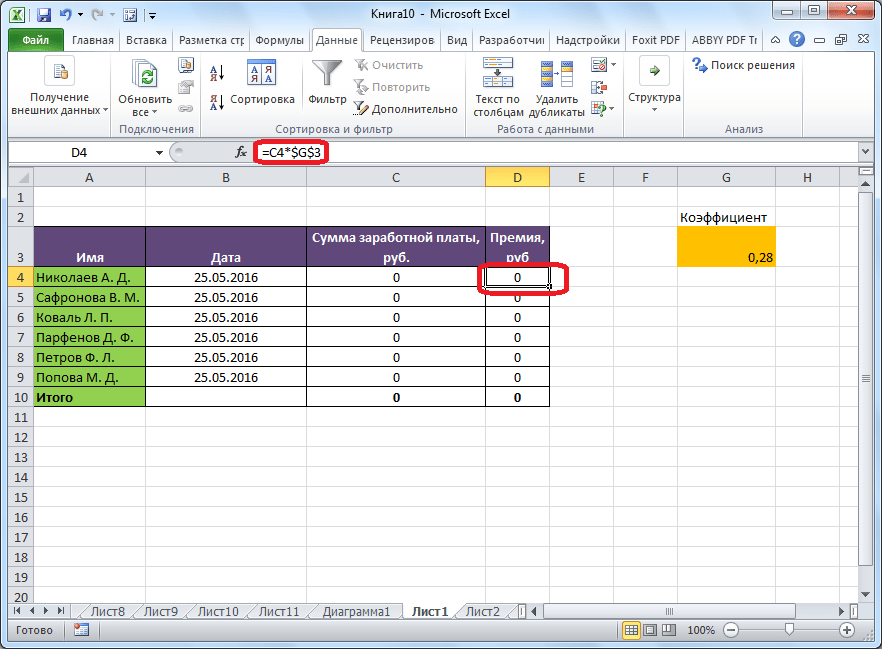
Имеем таблицу выплат заработной платы и премии работникам предприятия. Известны только премии работников. Например, премия одного из них — Николаева А. Д, составляет 6035,68 рублей. Также, известно, что премия рассчитывается путем умножения заработной платы на коэффициент 0,28. Нам предстоит найти заработную плату работников.
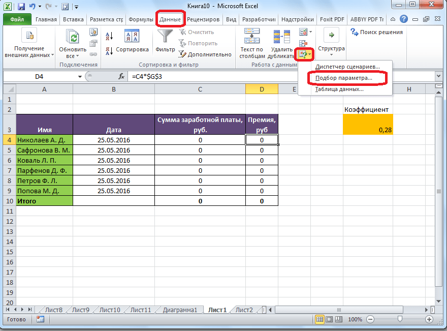
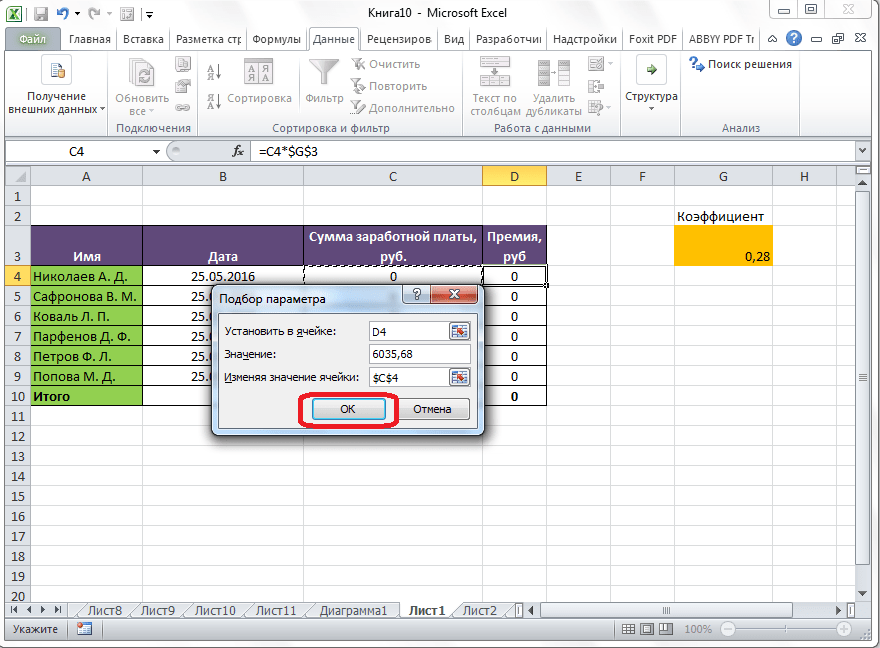
Для того, чтобы запустить функцию, находясь во вкладке «Данные», жмем на кнопку «Анализ «что если»», которая расположена в блоке инструментов «Работа с данными» на ленте. Появляется меню, в котором нужно выбрать пункт «Подбор параметра…».
После этого, открывается окно подбора параметра. В поле «Установить в ячейке» нужно указать ее адрес, содержащей известные нам конечные данные, под которые мы будем подгонять расчет. В данном случае, это ячейка, где установлена премия работника Николаева. Адрес можно указать вручную, вбив его координаты в соответствующее поле. Если вы затрудняетесь, это сделать, или считаете неудобным, то просто кликните по нужной ячейке, и адрес будет вписан в поле.
В поле «Значение» требуется указать конкретное значение премии. В нашем случае, это будет 6035,68. В поле «Изменяя значения ячейки» вписываем ее адрес, содержащей исходные данные, которые нам нужно рассчитать, то есть сумму зарплаты работника. Это можно сделать теми же способами, о которых мы говорили выше: вбить координаты вручную, или кликнуть по соответствующей ячейке.
Когда все данные окна параметров заполнены, жмем на кнопку «OK».
После этого, совершается расчет, и в ячейки вписываются подобранные значения, о чем сообщает специальное информационное окно.
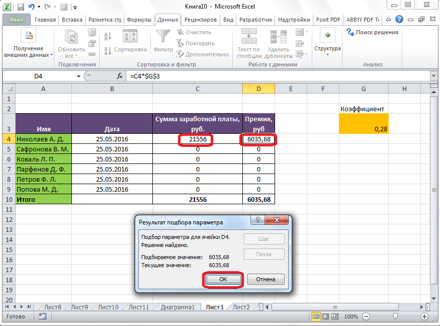
Подобную операцию можно проделать и для других строк таблицы, если известна величина премии остальных сотрудников предприятия.

Решение уравнений
Кроме того, хотя это и не является профильной возможностью данной функции, её можно использовать для решения уравнений. Правда, инструмент подбора параметра можно с успехом использовать только относительно уравнений с одним неизвестным.
Допустим, имеем уравнение: 15x+18x=46. Записываем его левую часть, как формулу, в одну из ячеек. Как и для любой формулы в Экселе, перед уравнением ставим знак «=». Но, при этом, вместо знака x устанавливаем адрес ячейки, куда будет выводиться результат искомого значения.
В нашем случае, формулу мы запишем в C2, а искомое значение будет выводиться в B2. Таким образом, запись в ячейке C2 будет иметь следующий вид: «=15*B2+18*B2».

Запускаем функцию тем же способом, как было описано выше, то есть, нажав на кнопку «Анализ «что если»» на ленте», и перейдя по пункту «Подбор параметра…».

В открывшемся окне подбора параметра, в поле «Установить в ячейке» указываем адрес, по которому мы записали уравнение (C2). В поле «Значение» вписываем число 45, так как мы помним, что уравнение выглядит следующим образом: 15x+18x=46. В поле «Изменяя значения ячейки» мы указываем адрес, куда будет выводиться значение x, то есть, собственно, решение уравнения (B2). После того, как мы ввели эти данные, жмем на кнопку «OK».

Как видим, программа Microsoft Excel успешно решила уравнение. Значение x будет равно 1,39 в периоде.

Изучив инструмент Подбор параметра, мы выяснили, что это довольно простая, но вместе с тем полезная и удобная функция для поиска неизвестного числа. Её можно использовать как для табличных вычислений, так и для решения уравнений с одним неизвестным. Вместе с тем, по функционалу она уступает более мощному инструменту Поиск решения.