
If you know the result that you want from a formula, but are not sure what input value the formula needs to get that result, use the Goal Seek feature. For example, suppose that you need to borrow some money. You know how much money you want, how long you want to take to pay off the loan, and how much you can afford to pay each month. You can use Goal Seek to determine what interest rate you will need to secure in order to meet your loan goal.
If you know the result that you want from a formula, but are not sure what input value the formula needs to get that result, use the Goal Seek feature. For example, suppose that you need to borrow some money. You know how much money you want, how long you want to take to pay off the loan, and how much you can afford to pay each month. You can use Goal Seek to determine what interest rate you will need to secure in order to meet your loan goal.
Note: Goal Seek works only with one variable input value. If you want to accept more than one input value; for example, both the loan amount and the monthly payment amount for a loan, you use the Solver add-in. For more information, see Define and solve a problem by using Solver.
Step-by-step with an example
Let’s look at the preceding example, step-by-step.
Because you want to calculate the loan interest rate needed to meet your goal, you use the PMT function. The PMT function calculates a monthly payment amount. In this example, the monthly payment amount is the goal that you seek.
Prepare the worksheet
-
Open a new, blank worksheet.
-
First, add some labels in the first column to make it easier to read the worksheet.
-
In cell A1, type Loan Amount.
-
In cell A2, type Term in Months.
-
In cell A3, type Interest Rate.
-
In cell A4, type Payment.
-
-
Next, add the values that you know.
-
In cell B1, type 100000. This is the amount that you want to borrow.
-
In cell B2, type 180. This is the number of months that you want to pay off the loan.
Note: Although you know the payment amount that you want, you do not enter it as a value, because the payment amount is a result of the formula. Instead, you add the formula to the worksheet and specify the payment value at a later step, when you use Goal Seek.
-
-
Next, add the formula for which you have a goal. For the example, use the PMT function:
-
In cell B4, type =PMT(B3/12,B2,B1). This formula calculates the payment amount. In this example, you want to pay $900 each month. You don’t enter that amount here, because you want to use Goal Seek to determine the interest rate, and Goal Seek requires that you start with a formula.
The formula refers to cells B1 and B2, which contain values that you specified in preceding steps. The formula also refers to cell B3, which is where you will specify that Goal Seek put the interest rate. The formula divides the value in B3 by 12 because you specified a monthly payment, and the PMT function assumes an annual interest rate.
Because there is no value in cell B3, Excel assumes a 0% interest rate and, using the values in the example, returns a payment of $555.56. You can ignore that value for now.
-
Use Goal Seek to determine the interest rate
-
On the Data tab, in the Data Tools group, click What-If Analysis, and then click Goal Seek.
-
In the Set cell box, enter the reference for the cell that contains the formula that you want to resolve. In the example, this reference is cell B4.
-
In the To value box, type the formula result that you want. In the example, this is -900. Note that this number is negative because it represents a payment.
-
In the By changing cell box, enter the reference for the cell that contains the value that you want to adjust. In the example, this reference is cell B3.
Note: The cell that Goal Seek changes must be referenced by the formula in the cell that you specified in the Set cell box.
-
Click OK.
Goal Seek runs and produces a result, as shown in the following illustration.

Cells B1, B2, and B3 are the values for the loan amount, term length, and interest rate.
Cell B4 displays the result of the formula =PMT(B3/12,B2,B1).
-
Finally, format the target cell (B3) so that it displays the result as a percentage.
-
On the Home tab, in the Number group, click Percentage.
-
Click Increase Decimal or Decrease Decimal to set the number of decimal places.
-

If you know the result that you want from a formula, but are not sure what input value the formula needs to get that result, use the Goal Seek feature. For example, suppose that you need to borrow some money. You know how much money you want, how long you want to take to pay off the loan, and how much you can afford to pay each month. You can use Goal Seek to determine what interest rate you will need to secure in order to meet your loan goal.
Note: Goal Seek works only with one variable input value. If you want to accept more than one input value, for example, both the loan amount and the monthly payment amount for a loan, use the Solver add-in. For more information, see Define and solve a problem by using Solver.
Step-by-step with an example
Let’s look at the preceding example, step-by-step.
Because you want to calculate the loan interest rate needed to meet your goal, you use the PMT function. The PMT function calculates a monthly payment amount. In this example, the monthly payment amount is the goal that you seek.
Prepare the worksheet
-
Open a new, blank worksheet.
-
First, add some labels in the first column to make it easier to read the worksheet.
-
In cell A1, type Loan Amount.
-
In cell A2, type Term in Months.
-
In cell A3, type Interest Rate.
-
In cell A4, type Payment.
-
-
Next, add the values that you know.
-
In cell B1, type 100000. This is the amount that you want to borrow.
-
In cell B2, type 180. This is the number of months that you want to pay off the loan.
Note: Although you know the payment amount that you want, you do not enter it as a value, because the payment amount is a result of the formula. Instead, you add the formula to the worksheet and specify the payment value at a later step, when you use Goal Seek.
-
-
Next, add the formula for which you have a goal. For the example, use the PMT function:
-
In cell B4, type =PMT(B3/12,B2,B1). This formula calculates the payment amount. In this example, you want to pay $900 each month. You don’t enter that amount here, because you want to use Goal Seek to determine the interest rate, and Goal Seek requires that you start with a formula.
The formula refers to cells B1 and B2, which contain values that you specified in preceding steps. The formula also refers to cell B3, which is where you will specify that Goal Seek put the interest rate. The formula divides the value in B3 by 12 because you specified a monthly payment, and the PMT function assumes an annual interest rate.
Because there is no value in cell B3, Excel assumes a 0% interest rate and, using the values in the example, returns a payment of $555.56. You can ignore that value for now.
-
Use Goal Seek to determine the interest rate
-
Do one of the following:
In Excel 2016 for Mac: On the Data tab, click What-If Analysis, and then click Goal Seek.
In Excel for Mac 2011: On the Data tab, in the Data Tools group, click What-If Analysis, and then click Goal Seek.
-
In the Set cell box, enter the reference for the cell that contains the formula that you want to resolve. In the example, this reference is cell B4.
-
In the To value box, type the formula result that you want. In the example, this is -900. Note that this number is negative because it represents a payment.
-
In the By changing cell box, enter the reference for the cell that contains the value that you want to adjust. In the example, this reference is cell B3.
Note: The cell that Goal Seek changes must be referenced by the formula in the cell that you specified in the Set cell box.
-
Click OK.
Goal Seek runs and produces a result, as shown in the following illustration.
-
Finally, format the target cell (B3) so that it displays the result as a percentage. Follow one of these steps:
-
In Excel 2016 for Mac: On the Home tab, click Increase Decimal
or Decrease Decimal . -
In Excel for Mac 2011: On the Home tab, under Number group, click Increase Decimal
or Decrease Decimal to set the number of decimal places.
-
 or Decrease Decimal
  .
. or Decrease Decimal
  to set the number of decimal places.
Очень полезной функцией в программе Microsoft Excel является Подбор параметра. Но, далеко не каждый пользователь знает о возможностях данного инструмента. С его помощью, можно подобрать исходное значение, отталкиваясь от конечного результата, которого нужно достичь. Давайте выясним, как можно использовать функцию подбора параметра в Microsoft Excel.
Суть функции
Если упрощенно говорить о сути функции Подбор параметра, то она заключается в том, что пользователь, может вычислить необходимые исходные данные для достижения конкретного результата. Эта функция похожа на инструмент Поиск решения, но является более упрощенным вариантом. Её можно использовать только в одиночных формулах, то есть для вычисления в каждой отдельной ячейке нужно запускать всякий раз данный инструмент заново. Кроме того, функция подбора параметра может оперировать только одним вводным, и одним искомым значением, что говорит о ней, как об инструменте с ограниченным функционалом.
Применение функции на практике
Для того, чтобы понять, как работает данная функция, лучше всего объяснить её суть на практическом примере. Мы будем объяснять работу инструмента на примере программы Microsoft Excel 2010, но алгоритм действий практически идентичен и в более поздних версиях этой программы, и в версии 2007 года.
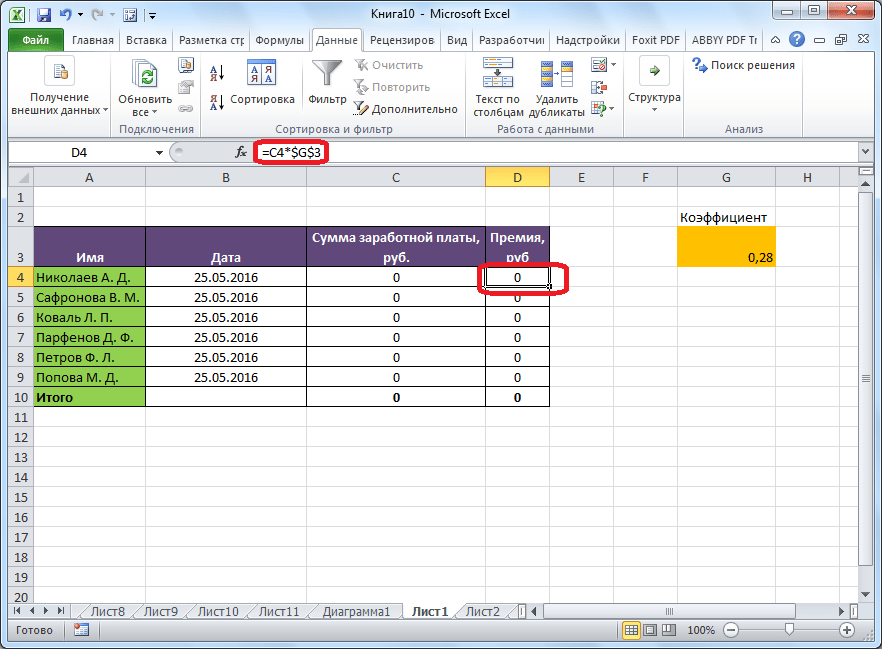
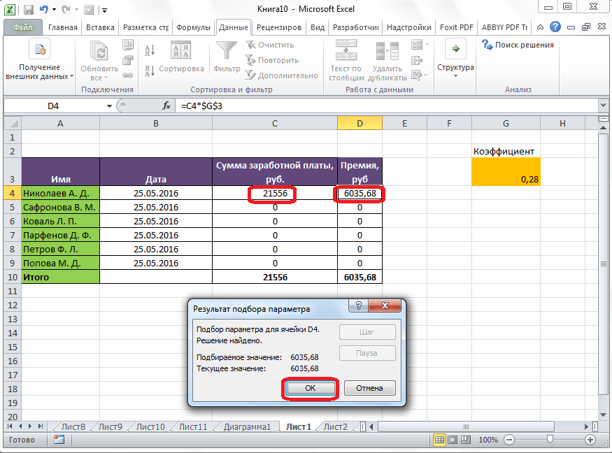
Имеем таблицу выплат заработной платы и премии работникам предприятия. Известны только премии работников. Например, премия одного из них — Николаева А. Д, составляет 6035,68 рублей. Также, известно, что премия рассчитывается путем умножения заработной платы на коэффициент 0,28. Нам предстоит найти заработную плату работников.
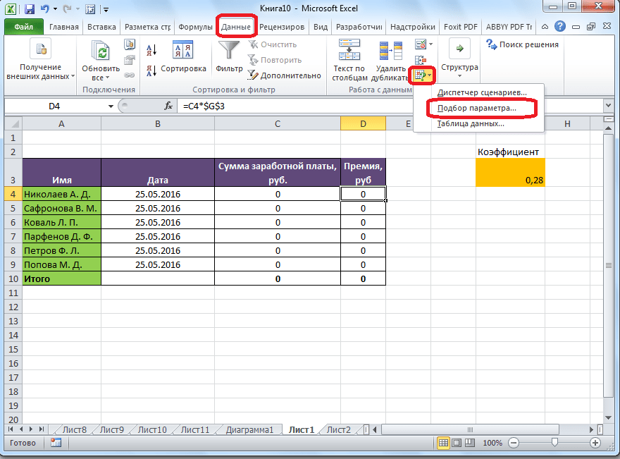
Для того, чтобы запустить функцию, находясь во вкладке «Данные», жмем на кнопку «Анализ «что если»», которая расположена в блоке инструментов «Работа с данными» на ленте. Появляется меню, в котором нужно выбрать пункт «Подбор параметра…».
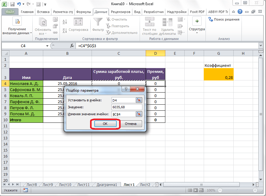
После этого, открывается окно подбора параметра. В поле «Установить в ячейке» нужно указать ее адрес, содержащей известные нам конечные данные, под которые мы будем подгонять расчет. В данном случае, это ячейка, где установлена премия работника Николаева. Адрес можно указать вручную, вбив его координаты в соответствующее поле. Если вы затрудняетесь, это сделать, или считаете неудобным, то просто кликните по нужной ячейке, и адрес будет вписан в поле.
В поле «Значение» требуется указать конкретное значение премии. В нашем случае, это будет 6035,68. В поле «Изменяя значения ячейки» вписываем ее адрес, содержащей исходные данные, которые нам нужно рассчитать, то есть сумму зарплаты работника. Это можно сделать теми же способами, о которых мы говорили выше: вбить координаты вручную, или кликнуть по соответствующей ячейке.
Когда все данные окна параметров заполнены, жмем на кнопку «OK».
После этого, совершается расчет, и в ячейки вписываются подобранные значения, о чем сообщает специальное информационное окно.
Подобную операцию можно проделать и для других строк таблицы, если известна величина премии остальных сотрудников предприятия.

Решение уравнений
Кроме того, хотя это и не является профильной возможностью данной функции, её можно использовать для решения уравнений. Правда, инструмент подбора параметра можно с успехом использовать только относительно уравнений с одним неизвестным.
Допустим, имеем уравнение: 15x+18x=46. Записываем его левую часть, как формулу, в одну из ячеек. Как и для любой формулы в Экселе, перед уравнением ставим знак «=». Но, при этом, вместо знака x устанавливаем адрес ячейки, куда будет выводиться результат искомого значения.
В нашем случае, формулу мы запишем в C2, а искомое значение будет выводиться в B2. Таким образом, запись в ячейке C2 будет иметь следующий вид: «=15*B2+18*B2».

Запускаем функцию тем же способом, как было описано выше, то есть, нажав на кнопку «Анализ «что если»» на ленте», и перейдя по пункту «Подбор параметра…».

В открывшемся окне подбора параметра, в поле «Установить в ячейке» указываем адрес, по которому мы записали уравнение (C2). В поле «Значение» вписываем число 45, так как мы помним, что уравнение выглядит следующим образом: 15x+18x=46. В поле «Изменяя значения ячейки» мы указываем адрес, куда будет выводиться значение x, то есть, собственно, решение уравнения (B2). После того, как мы ввели эти данные, жмем на кнопку «OK».

Как видим, программа Microsoft Excel успешно решила уравнение. Значение x будет равно 1,39 в периоде.

Изучив инструмент Подбор параметра, мы выяснили, что это довольно простая, но вместе с тем полезная и удобная функция для поиска неизвестного числа. Её можно использовать как для табличных вычислений, так и для решения уравнений с одним неизвестным. Вместе с тем, по функционалу она уступает более мощному инструменту Поиск решения.
A what-if analysis tool used to find the value of an assumption based on the desired output
What is the Goal Seek Excel Tool?
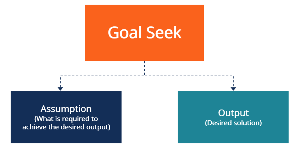
The Goal Seek[1] Excel tool is a form of what-if analysis that tells us what value an assumption needs to be in order to reach a desired output or result. It is a form of reverse engineering, where the user starts with the outcome and answer that they want and Excel works backward to find out what’s required. It is commonly used in financial modeling and other types of financial analysis.
Learn more in CFI’s Advanced Excel Formulas Course.
How to Use the Goal Seek Excel Tool (Example)
Follow this step-by-step guide on how to use Goal Seek to understand the cause and effect relationships between inputs and outputs in an Excel model:
Step #1
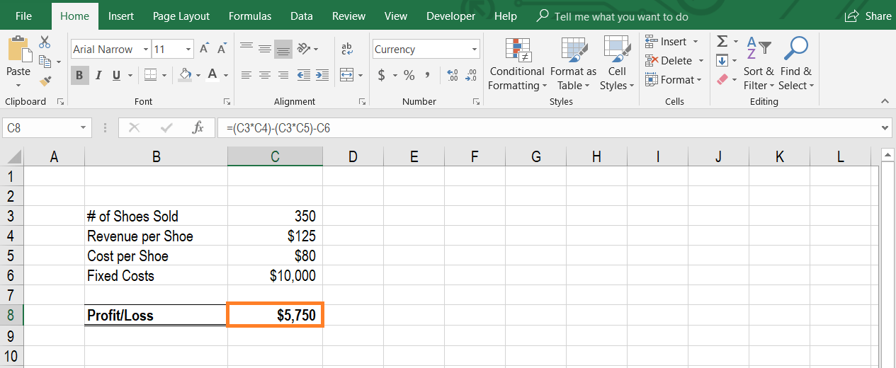
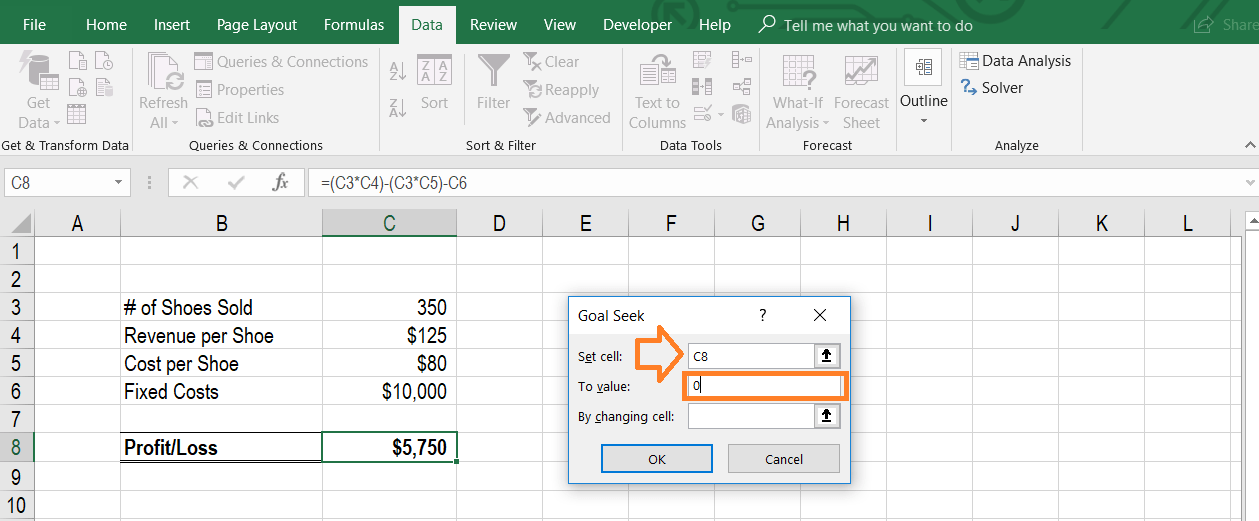
Navigate to the cell that contains the output or result you want to analyze. In this case, we have a simple model that examines how much profit/loss a shoe retailer makes depending on how many shoes they sell. We want to see how many shoes they need to sell to break even (generate exactly zero profit/loss). To run this test, we put the cursor in cell C8.
Step #2
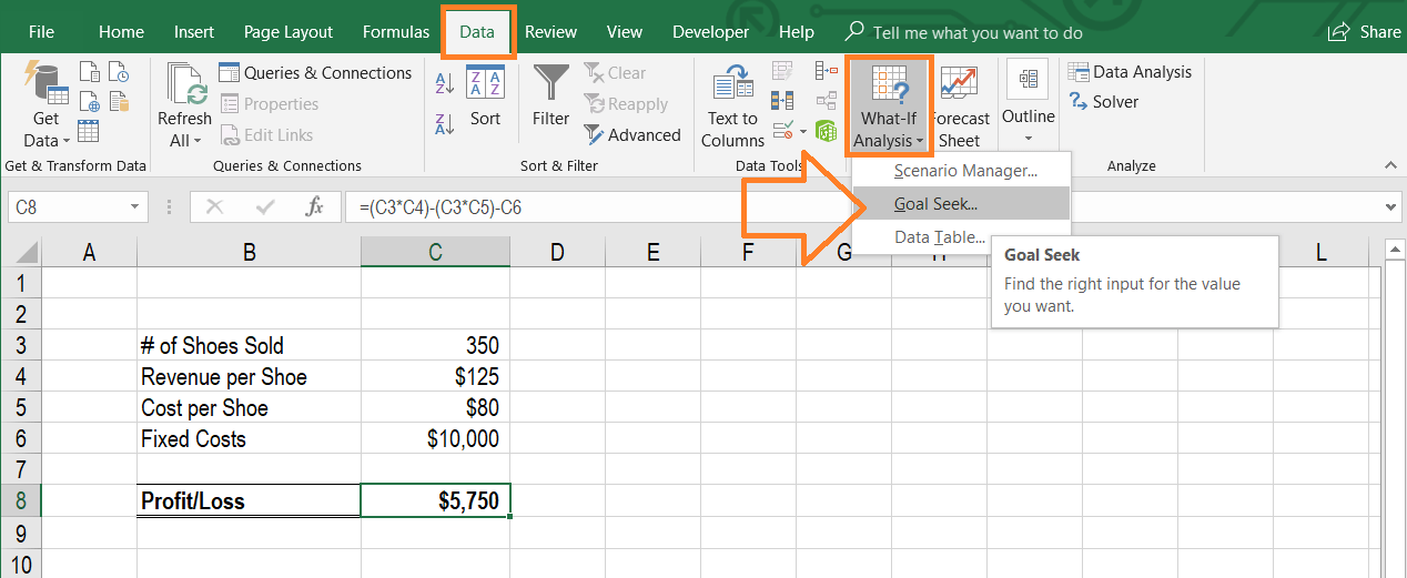
Open Goal Seek by accessing the Data section of the ribbon, then select What-If Analysis and then click Goal Seek. The keyboard shortcut on Windows is Alt, A, W, G. When this is completed, the Goal Seek Excel dialogue box will appear.
Step #3
When the Goal Seek Excel dialogue box appears, link the cell that you want to set the value of and then enter the value you want it to be set to. In this case, we want to change the profit/loss value to zero. It means linking the Set Cell to C8 and the To Value to 0.
Step #4
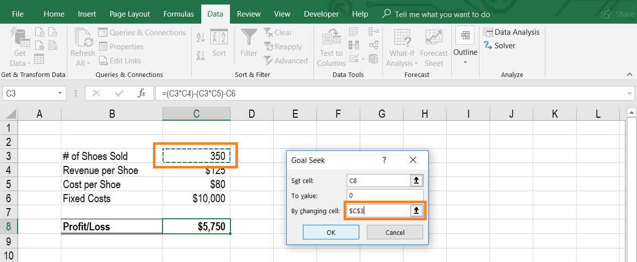
Link to the cell that you want Excel to change in order to generate the solution. Since we want to know how many shoes need to be sold in order to break even, we link the By Changing Cell to be C3. Then press OK.
Step #5
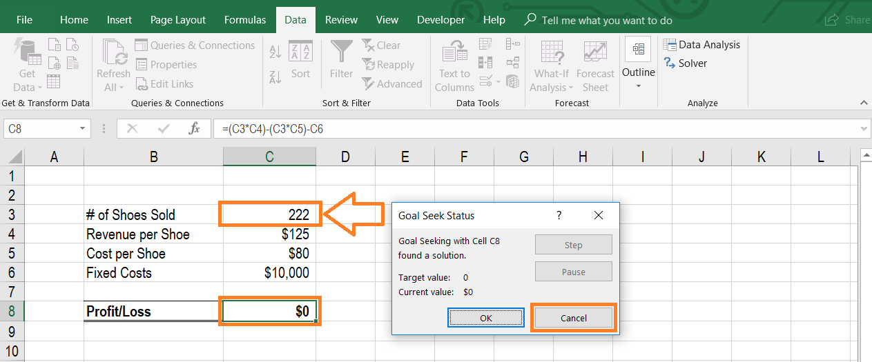
At this point, the solution will be displayed in the By Changing Cell and the Set Value Cell. In this case, we see that 222 shoes need to be sold (cell C3) to break-even with zero profit (cell C8).
If you wish to leave the results of the test in the spreadsheet, press OK. Note, this will change your model to now have the new values in it. If you simply wanted to take note of the solution, but return to your original numbers, press Cancel (this is the most common way to use Goal Seek).
Why Use the Goal Seek Excel Function?
There are many reasons to use the Goal Seek Excel function, especially when performing financial modeling and analysis.
Common reasons include:
- Break-even analysis
- Scenario analysis
- Sensitivity analysis
- Understanding cause and effect
- Answering specific questions (e.g., how many shoes do we need to sell to earn $2,500 in profit?)
- Stress testing a model
Video Explanation of Goal Seek
Below is a short video that will show you exactly how to use this function in your spreadsheets. Watch the demonstration and start using the function on your own.
Additional Resources
Thank you for reading CFI’s guide to the Goal Seek Excel function, how to use it, and why it matters. To continue learning and advancing your career as a financial analyst, you will find these additional CFI resources helpful.
- Advanced Excel Formulas
- Excel Modeling Best Practices
- Scenario Analysis
- Valuation Modeling in Excel
- See all Excel resources
Article Sources
- Goal Seek
Got the output for a formula but don’t know the input? Back-solving with Goal Seek might be just what you need.

Excel’s What-If Analysis allows you to see how changing a cell can affect a formula’s output. You can use Excel’s tools for this purpose to calculate the effect of changing the value of a cell in a formula.
Excel has three types of What-If Analysis tools: Scenario Manager, Goal Seek, and Data Table. With Goal Seek, you can determine what input you need to convert the formula backward to a certain output.
The Goal Seek feature in Excel is trial and error, so if it does not produce what you want, then Excel works on improving that value until it does.
What Are Excel Goal Seek Formulas?
Goal Seek in Excel essentially breaks down into three major components:
- Set cell: The cell you want to use as your goal.
- To value: The value you want as your goal.
- By changing cell: The cell you would like to change to reach your goal value.
With these three settings set, Excel will attempt to improve the value in the cell you set in By changing cell until the cell you set in Set cell reaches the value you determined in To value.
If all that sounds confusing, the examples below will give you a good idea of how Goal Seek works.
Goal Seek Example 1
For instance, let’s say you have two cells (A & B) and a third cell that calculates the average of these two.
Now suppose you have a static value for A, and you wish to raise the average level by changing the value for B. By using Goal Seek, you can calculate what value of B will produce the average you want.
How to Use Goal Seek in Excel
- In Excel, click cell C1.
- In the formula bar, enter the following code:
=AVERAGE(A1:B1)This formula will have Excel calculate the average of the values in cells A1 and B1 and output that in cell C1. You can make sure your formula works by inputting numbers in A1 and B1. C1 should show their average.
- For this example, change the value of the A1 cell to 16.
- Select cell C1, and then from the ribbon, go to the Data tab.
- Under the Data tab, select What-If Analysis and then Goal Seek. This will bring up the Goal Seek window.
- In the Goal Seek window, set the Set cell to C1. This will be your goal cell. Having highlighted C1 before opening the Goal Seek window will automatically set it in Set cell.
- In To value, insert the goal value you want. For this example, we want our average to be 26, so the goal value will be 26 as well.
- Finally, in the By changing cell, select the cell you want to change to reach the goal. In this example, this will be cell B2.
- Click OK to have Goal Seek work its magic.
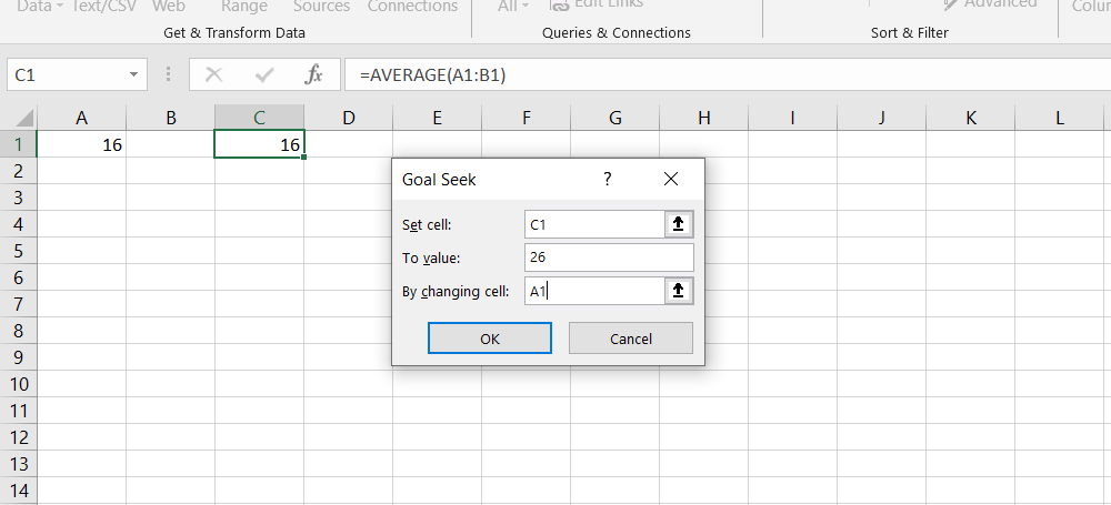
Once you click OK, a dialogue will appear informing you that Goal Seek has found a solution.
The value of cell A1 will change to the solution, and this will overwrite the previous data. It’s a good idea to run Goal Seek on a copy of your datasheet to avoid losing your original data.
Goal Seek Example 2
Goal Seek can be useful when you utilize it in real-life scenarios. However, to use Goal Seek to its full potential, you need to have a proper formula in place, to begin with.
For this example, let’s take a small banking case. Suppose that you have a bank account that gives you a 4% annual interest on the money you have in your account.
Using What-If Analysis and Goal Seek, you can calculate how much money you need to have in your account to get a certain amount of monthly interest payment.
For this example, let’s say we want to get $350 every month from interest payments. Here’s how you can calculate that:
- In cell A1 type Balance.
- In cell A2 type Annual Rate.
- In cell A4 type Monthly Profit.
- In cell B2 type 4%.
- Select cell B4 and in the formula bar, enter the formula below:
=B1*B2/12The monthly profit will equal the account balance multiplied by the annual rate and then divided by the number of months in a year, 12 months.
- Go to the Data tab, click on What-If Analysis, and then select Goal Seek.
- In the Goal Seek window, type B4 in Set cell.
- Type 350 in the To value cell. (This is the monthly profit you want to get)
- Type B1 in By changing cell. (This will change the balance to a value that will yield $350 monthly)
- Click OK. The Goal Seek Status dialogue will pop up.
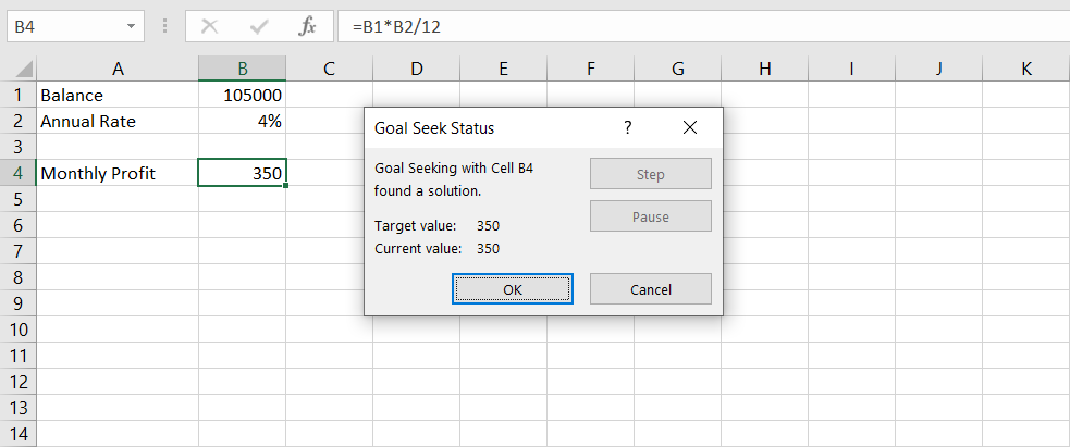
In the Goal Seeking Status dialog, you’ll see that Goal Seeking has found a solution in cell B4. In cell B1, you can see the solution, which should be 105,000.
Goal Seek Requirements
With Goal Seek, you can see that it can change only one cell to reach the goal value. This means that Goal Seek cannot solve and reach a solution if it has more than one variable.
In Excel, you can still solve for more than one variable, but you’ll need to use another tool called the Solver. You can read more about Excel’s Solver by reading our article on How To Use Excel’s Solver.
Goal Seek Limitations
A Goal Seek formula uses the trial-and-improvement process to reach the optimal value, which can pose some problems when the formula produces an undefined value. Here’s how you can test it yourself:
- In cell A1, type 3.
- Select cell C1, then in the formula bar enter the formula below:
=1/(A1-5)This formula will divide one by A1-5, and if A1-5 happens to be 0, the result will be an undefined value.
- Go to the Data tab, click What-If Analysis and then select Goal Seek.
- In Set cell, type C1.
- In To value, type 1.
- Finally, in By changing cell type A1. (This will change the A1 value to reach 1 in C1)
- Click OK.
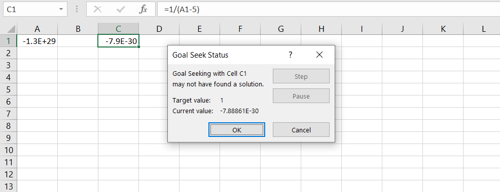
The Goal Seek Status dialogue box will tell you that it may not have found a solution, and you can double-check that the A1 value is way off.
Now, the solution to this Goal Seek would be to simply have 6 in A1. This will give 1/1, which equals 1. But at one point during the trial and improvement process, Excel tries 5 in A1, which gives 1/0, which is undefined, killing the process.
A way around this Goal Seek problem is to have a different starting value, one that can evade the undefined in the trial and improvement process.
As an example, if you change A1 to any number greater than 5 and then repeat the same steps to Goal Seek for 1, you should get the correct result.
Make the Calculations More Efficient With Goal Seek
What-If Analysis and Goal Seek can speed up your calculations with your formulas by a great measure. Learning the right formulas is another important step toward becoming an excel master.

Функция поиска цели в Excel позволяет вам отвечать на вопросы «что, если», используя данные Excel. Вот как это использовать.
Инструмент Goal Seek — это встроенная функция Excel, которая позволяет быстро ответить на важный вопрос — что, если? Вы можете узнать желаемый результат из формулы Excel, но не переменные, которые помогут вам в этом.
Поиск цели пытается помочь вам, находя правильную переменную, необходимую для достижения определенной цели. Это позволяет анализировать данные Excel, в которых некоторые переменные просто неизвестны, пока вы не воспользуетесь поиском цели. Вот как это использовать.
Эта функция доступна в версиях Microsoft Excel начиная с 2010 года, и приведенные ниже инструкции должны оставаться одинаковыми для всех версий.
Сколько продаж вам нужно, чтобы продукт достиг цели по продажам?
Вы можете решить это вручную, но вскоре это может стать сложным для более сложных запросов. Вместо этого вы можете использовать функцию поиска цели в Microsoft Excel, чтобы обдумать вопрос и найти целевой ответ.
Ведь математическая формула — это просто вопрос с ответом.
Этот тип анализа «что, если» требует, чтобы у вас было целевое значение, которого вы хотите достичь, а также текущее значение в ячейке, которое Excel может изменить, чтобы попытаться достичь целевого значения.
Например, для нашего примера дохода от продукта вам нужно указать количество продаж в ячейке. Затем вы можете использовать Поиск цели, используя целевой доход от продукта в качестве целевого значения, чтобы определить количество продаж, которое вам потребуется.
Затем Excel изменит значение (в данном случае, цель продаж), чтобы достичь целевого значения. Затем вы увидите предварительный просмотр результата — затем вы можете применить изменения к вашему листу или отменить их.
Как использовать поиск цели в Excel
Чтобы использовать инструмент поиска цели, откройте электронную таблицу Excel и нажмите Данные вкладка на панели ленты.
в Прогноз раздел Данные нажмите вкладку Что, если анализ кнопка. Появится раскрывающееся меню — нажмите Поиск цели вариант начать.
Поиск цели В окне есть три значения, которые вам нужно установить.
Установить ячейку это ячейка, содержащая вашу математическую формулу — вопрос без правильного ответа (в настоящее время). Используя наш пример продаж продукта, это будет формула цели продаж (1), который в настоящее время составляет 2500 долларов США.
в Ценить, оценивать поле, установите целевое значение. Для нашего примера продажи продукта это будет целевой доход (например, 10 000 долларов США).
Наконец, определите ячейку, содержащую изменяющуюся переменную в Меняя челL коробка (2). Для нашего примера это будет содержать текущее количество продаж. В настоящее время 100 продаж — это нужно изменить, чтобы достичь увеличенного целевого значения.
Поиск цели изменит это число (100 продаж), чтобы достичь целевого значения, установленного в Ценить, оценивать коробка.
нажмите ОК Нажмите кнопку, чтобы начать анализ поиска. Если поиск цели найдет подходящий ответ, который соответствует целевому значению, он отобразится в Статус поиска цели коробка.
В этом примере первоначальное число 100 продаж было увеличено до 400 продаж, чтобы достичь целевого значения в 10 000 долларов.
Если вы довольны ответом, который находит Поиск цели, нажмите ОК кнопка. В противном случае нажмите Отмена— это закроет окно «Поиск цели» и восстановит исходные значения.
Лучший анализ данных Excel
Использование функции поиска цели в Excel — отличный вариант, если вы упускаете некоторые части из математического вопроса. Однако существуют альтернативы поиску целей, в том числе надстройка Excel Solver.
Когда у вас есть данные, вы можете использовать функцию CONCATENATE в Excel, чтобы использовать ваши данные и представлять их для лучшего анализа данных в Excel. Однако, если вы новичок в Excel, вам нужно знать некоторые общие советы по Excel.