
Excel IF AND OR functions on their own aren’t very exciting, but mix them up with the IF Statement and you’ve got yourself a formula that’s much more powerful.
In this tutorial we’re going to take a look at the basics of the AND and OR functions and then put them to work with an IF Statement. If you aren’t familiar with IF Statements, click here to read that tutorial first.
IF Formula Builder
Our IF Formula Builder does the hard work of creating IF formulas.
You just need to enter a few pieces of information, and the workbook creates the formula for you.
AND Function
The AND function belongs to the logic family of formulas, along with IF, OR and a few others. It’s useful when you have multiple conditions that must be met.
In Excel language on its own the AND formula reads like this:
=AND(logical1,[logical2]....)
Now to translate into English:
=AND(is condition 1 true, AND condition 2 true (add more conditions if you want)
OR Function
The OR function is useful when you are happy if one, OR another condition is met.
In Excel language on its own the OR formula reads like this:
=OR(logical1,[logical2]....)
Now to translate into English:
=OR(is condition 1 true, OR condition 2 true (add more conditions if you want)
See, I did say they weren’t very exciting, but let’s mix them up with IF and put AND and OR to work.
IF AND Formula
First let’s set the scene of our challenge for the IF, AND formula:
In our spreadsheet below we want to calculate a bonus to pay the children’s TV personalities listed. The rules, as devised by my 4 year old son, are:
1) If the TV personality is Popular AND
2) If they earn less than $100k per year they get a 10% bonus (my 4 year old will write them an IOU, he’s good for it though).

In cell D2 we will enter our IF AND formula as follows:
In English first
=IF(Spider Man is Popular, AND he earns <$100k), calculate his salary x 10%, if not put "Nil" in the cell)
Now in Excel’s language:
=IF(AND(B2="Yes",C2<100),C2x$H$1,"Nil")
You’ll notice that the two conditions are typed in first, and then the outcomes are entered. You can have more than two conditions; in fact you can have up to 30 by simply separating each condition with a comma (see warning below about going overboard with this though).
IF OR Formula
Again let’s set the scene of our challenge for the IF, OR formula:
The revised rules, as devised by my 4 year old son, are:
1) If the TV personality is Popular OR
2) If they earn less than $100k per year they get a 10% bonus.

In cell D2 we will enter our IF OR formula as follows:
In English first
=IF(Spider Man is Popular, OR he earns <$100k), calculate his salary x 10%, if not put “Nil” in the cell)
Now in Excel’s language:
=IF(OR(B2="Yes",C2<100),C2x$H$1,"Nil")
Notice how a subtle change from the AND function to the OR function has a significant impact on the bonus figure.
Just like the AND function, you can have up to 30 OR conditions nested in the one formula, again just separate each condition with a comma.
Try other operators
You can set your conditions to test for specific text, as I have done in this example with B2=»Yes», just put the text you want to check between inverted comas “ ”.
Alternatively you can test for a number and because the AND and OR functions belong to the logic family, you can employ different tests other than the less than (<) operator used in the examples above.
Other operators you could use are:
- = Equal to
- > Greater Than
- <= Less than or equal to
- >= Greater than or equal to
- <> Less than or greater than
Warning: Don’t go overboard with nesting IF, AND, and OR’s, as it will be painful to decipher if you or someone else ever needs to update the formula in months or years to come.
Note: These formulas work in all versions of Excel, however versions pre Excel 2007 are limited to 7 nested IF’s.
Download the Workbook
Enter your email address below to download the sample workbook.
By submitting your email address you agree that we can email you our Excel newsletter.
Excel IF AND OR Practice Questions
IF AND Formula Practice
In the embedded Excel workbook below insert a formula (in the grey cells in column E), that returns the text ‘Yes’, when a product SKU should be reordered, based on the following criteria:
- If Stock on hand is less than 20,000 AND
- Demand level is ‘High’
If the above conditions are met, return ‘Yes’, otherwise, return ‘No’.
Tips for working with the embedded workbook:
- Use arrow keys to move around the worksheet when you can’t click on the cells with your mouse
- Use shortcut keys CTRL+C to copy and CTRL+V to paste
- Don’t forget to absolute cell references where applicable
- Do not enter anything in column F
- Double click to edit a cell
- Refresh the page to reset the embedded workbook
IF OR Formula Practice
In the embedded Excel workbook below insert a formula (in the grey cells in column E) that calculates the bonus due for each salesperson. A $500 bonus is paid if a salesperson meets either target in cells C24 and C25, otherwise they earn $0 bonus.
Want More Excel Formulas
Why not visit our list of Excel formulas. You’ll find a huge range all explained in plain English, plus PivotTables and other Excel tools and tricks. Enjoy 🙂
![]()
April 30, 2012 / Updated: October 24, 2021 / Lena Shore
Filed under: Tutorials
This tip is going to be mostly helpful to people who working with databases. But, if you work with Excel and find yourself needing to deal with repetitive formatting, you might also appreciate the technique.
When working with CSV files you may need to add quotes to either side of a cell’s contents in order to upload them properly to your database. You can easily find yourself working with an Excel file from a workmate that needs to be formatted.
You got this:

But really need this:

This can be a big damn deal if you have hundreds of fields. No one wants to add this by hand. Fortunately, the solution is a snap! It all has to do with applying specific formatting to your cells.
- Highlight the cells you want to add the quotes.
- Go to Format –> Cells –> Custom
- Copy/Paste the following into the Type field: ”@”
- Click “okay”
- Be happy you didn’t do it all by hand.
NOTE: It’s always a good idea to open your file in a text editor to double-check your CSV export. Sometimes you need to do a little find/replace action to get your file picture perfect.

Lena is a full-time freelancer and nerd that specializes in web development, graphic design, and illustration. She enjoys building things, learning new things, pursuing creative endeavors, and giving free advice.
Skip to content
![]()
Microsoft quietly replaced the comfortable Text Import Wizard from Excel and replaced it with the “Get & Transform” tools. The “Get & Transform” tools offer a lot of options and are very powerful. Unfortunately, they are quite complicated to use. Here is what you should now.
In a hurry? Click on “File” –> “Options” –> “Data” and set the corresponding checkmarks for reactivating the “Text Import Wizard” in Excel. Start the text import by clicking on “Data” –>”Get Data” –> “Legacy Wizards” –> “From Text (Legacy)”.
Introduction
In Excel 365 (only) 2016 (since version 1704) the “Text Import Wizard” was removed. It was replaced by the powerful “Get & Transform” tools. The “Get & Transform” tools also provide a function to import text and CSV files into Excel.
You have the following two options:
- Luckily, the comfortably “Text Import Wizard” still exists. You can re-activate and use it for importing text and csv files into Excel.
- Use the import function of the “Get & Transform” tools.
Restore the “Text Import Wizard”
The good news: You can easily restore the “Text Import Wizard”. Unfortunately, the option for re-activating them is hidden.
Follow these steps:
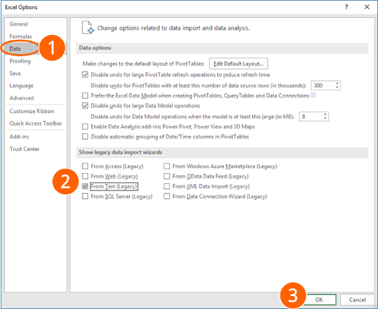
- Click on File and then on “Options”. Go to “Data” on the left-hand side.
- In the lower section of the window you can select the wizard you’d like to restore. For only importing text- or csv-files, select “From Text (Legacy)”. Feel free to also activate the corresponding wizard for importing Access files, files from web, from SQL servers and so on.
- Confirm with OK.
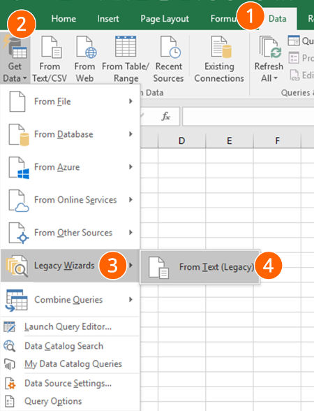
Now, you can find the so-called “Legacy Wizards” in the “Get Data” drop-down menu. In order to use them, follow these steps:
- Go to the “Data” ribbon.
- Click on “Get Data” on the left-hand side.
- Next, go to “Legacy Wizards”.
- Click on “From Text (Legacy)”.
How to use the “Text Import Wizard”
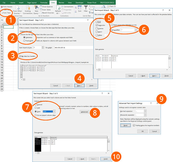
The steps for using the “Text Import Wizard” in Excel are shown in the screenshots.
- Go to the “Data” ribbon and click on “From Text”. If you have a recent Excel version and there is no button called “From Text” (but instead “From Text/CSV”), click on “Get Data”, then on “Legacy Wizards” and then on “From Text (Legacy)”. Please refer to the paragraph above if this option is missing.
- Select how you want to define the columns: Either with a character as a separator or with a fixed width.
- If the first row contains headers, check the corresponding box.
- Continue with “Next >”.
- Select the delimiter. This is the character dividing the data into columns, for example “Tab”, “Semicolon” or “Comma”.
- Usually text fields use quotation marks marking the beginning and end of a text field.
- For each column, you can choose the data format. For dates, you could define the order of days, months and years.
- Click on “Advanced”…
- …for defining decimals and thousands separators.
- Finalize the import by clicking on “Finish”.
Import text and csv files with the “Get & Transform” tools
Importing text files in Excel with the “Get & Transform” tools requires many steps. Please refer to the numbers on the screenshots:
- Click on “From Text/CSV” on the “Data” ribbon in order to start the import process.
- Choose the delimiter (e.g. semi-colon, comma etc.). Here you can also switch to “Fixed Width”. If you want to separate your import data with the “Fixed Width” option, you have to type the numbers of characters, after which you want to data to be divided.
- For further options (e.g. switching thousands- and decimal separators) click on “Edit”.
- If you data is not represented correctly, delete the automatically created step “Changed Type”.
- Change the date format: Right-click on a column that contains a date. Alternatively click on the small “ABC” symbol in the top left corner of the column heading.
- Move the mouse to “Change Type”.
- Click on “Using Locale…”.
- Select “Date”.
- Select the locale format for dates. In this example, the German date format is used.
- Confirm with OK. Repeat the steps 5 to 10 for each date column.
Recommendation: Select several date columns at the same time by pressing and holding the Ctrl key while selecting the columns. - Change the decimal and thousand separators: Right-click again on a column with decimal numbers.
- Move the mouse to “Change Type”.
- Click on “Using Local…”.
- Choose “Decimal Number”.
- Select the local number format. Please refer to this article for a list of local number formats.
- Confirm with “OK”.
- Last step: Insert the data into a worksheet. In order to achieve this, click on “Close & Load” in the top-left corner.

Henrik Schiffner is a freelance business consultant and software developer. He lives and works in Hamburg, Germany. Besides being an Excel enthusiast he loves photography and sports.
We use cookies on our website to give you the most relevant experience by remembering your preferences and repeat visits. By clicking “Accept”, you consent to the use of ALL the cookies.
.
Note: Video of solution at bottom of post.
A client of mine recently ran into an issue I hadn’t seen before. When she would click a formula cell and drag down to calculate it across multiple rows, it only copied the value. The formulas were correct, but the value being shown was from the original cell:
Somehow, sheet calculation had been set to manual. To fix this issue:
- Click on “Formulas” from the ribbon menu

- Expand “Calculation options”

- Change “Manual” to automatic


All of your calculations should now be done correctly.
Additional troubleshooting
If you’re still having an issue with drag-to-fill, make sure your advanced options (File –> Options –> Advanced) have “Enable fill handle…” checked.
You might also run into drag-to-fill issues if you’re filtering. Try removing all filters and dragging again.
We use the IF statement in Excel to test one condition and return one value if the condition is met and another if the condition is not met.
However, we use multiple or nested IF statements when evaluating numerous conditions in a specific order to return different results.
This tutorial shows four examples of using nested IF statements in Excel and gives five alternatives to using multiple IF statements in Excel.
General Syntax of Nested IF Statements (Multiple IF Statements)
The general syntax for nested IF statements is as follows:
=IF(Condition1, Value_if_true1, IF(Condition2, Value_if_true2, IF(Condition3, Value_if_true3, Value_if_false)))
This formula tests the first condition; if true, it returns the first value.
If the first condition is false, the formula moves to the second condition and returns the second value if it’s true.
Each subsequent IF function is incorporated into the value_if_false argument of the previous IF function.
This process continues until all conditions have been evaluated, and the formula returns the final value if none of the conditions is true.
The maximum number of nested IF statements allowed in Excel is 64.
Now, look at the following four examples of how to use nested IF statements in Excel.
Example #1: Use Multiple IF Statements to Assign Letter Grades Based on Numeric Scores
Let’s consider the following dataset showing some students’ scores on a Math test.

We want to use nested IF statements to assign student letter grades based on their scores.
We use the following steps:
- Select cell C2 and type in the below formula:
=IF(B2>=90,"A",IF(B2>=80,"B",IF(B2>=70,"C",IF(B2>=60,"D","F"))))

- Click Enter in the cell to get the result of the formula in the cell.
- Copy the formula for the rest of the cells in the column
The assigned letter grades appear in column C.

Explanation of the formula
=IF(B2>=90,”A”,IF(B2>=80,”B”,IF(B2>=70,”C”,IF(B2>=60,”D”,”F”))))
This formula evaluates the value in cell B2 and assigns an “A” if the value is 90 or greater, a “B” if the value is between 80 and 89, a “C” if the value is between 70 and 79, a “D” if the value is between 60 and 69, and an “F” if the value is less than 60.
Notice that it can be challenging to keep track of which parentheses go with which arguments in nested IF functions.
Therefore, as we enter the formula, Excel uses different colors for the parentheses at each level of the nested IF functions to make it easier to see which parts of the formula belong together.

Also read: How to use Excel If Statement with Multiple Conditions Range
Example #2: Use Multiple IF Statements to Calculate Commission Based on Sales Volume
Here’s the dataset showing the sales of specific salespeople in a particular month.

We want to use multiple IF statements to calculate the tiered commission for the salespeople based on their sales volume.
We proceed as follows:
- Select cell C2 and enter the following formula:
=IF(B2>=40000, B2*0.14,IF(B2>=20000,B2*0.12,IF(B2>=10000,B2*0.105,IF(B2>0,B2*0.08,0))))

- Press the Enter key to get the result of the formula.
- Double-click or drag the Fill Handle to copy the formula down the column.
The commission for each salesperson is displayed in column D.

Explanation of the formula
=IF(B2>=40000, B2*0.14,IF(B2>=20000,B2*0.12,IF(B2>=10000,B2*0.105,IF(B2>0,B2*0.08,0))))
This formula evaluates the value in cell B2 and then does the following:
- If the value in cell B2 is greater than or equal to 40,000, the figure is multiplied by 14% (0.14).
- If the figure in cell B2 is less than 40,000 but greater than or equal to 20,000, the value is multiplied by 12% (0.12).
- If the number in cell B2 is less than 20,000 but greater than or equal to 10,000, the figure is multiplied by 10.5% (0.105).
- If the value in cell B2 is less than 10,000 but greater than 0 (zero), the number is multiplied by 8% (0.08).
- If the value in cell B2 is 0 (zero), 0 (zero) is returned.
Example #3: Use Multiple IF Statements to Assign Sales Performance Rating Based On Sales Target Achievement
The following is a dataset showing regional sales data of a specific technology company in a particular year.

We want to use multiple IF statements to assign a sales performance rating to each region based on their sales target achievement.
We use the following steps:
- Select cell C2 and type in the below formula:
=IF(B2>500000, "Excellent", IF(B2>400000, "Good", IF(B2>275000, "Average", "Poor")))

- Click Enter on the Formula bar.
- Drag or double-click the Fill Handle to copy the formula down the column.
The performance ratings of the regions are shown in column C.

Explanation of the formula
=IF(B2>500000, “Excellent”, IF(B2>400000, “Good”, IF(B2>275000, “Average”, “Poor”)))
In this formula, if the sales target in cell B2 is greater than 500,000, the formula returns “Excellent.”
If it’s between 400,000 and 500,000, the formula returns “Good.”
If it’s between 275,000 and 400,000, the formula returns “Average.” And if it’s below 275,000, the formula returns “Poor.”
Example #4: Use Multiple IF Statements in Excel to Check For Errors and Return Error Messages
Suppose we have the following dataset of students’ English test scores. Some scores are less than 0 or greater than 100, and there are no scores in some cases.

We want to use nested IF statements to check for scores in column B and display error messages in column C if there are no scores or the scores are less than 0 or greater than 100.
If the score in column B is valid, we want the formula to return an empty string in column C.
Here are the steps to follow:
- Select cell C2 and enter the following formula:
=IF(OR(B2<0,B2>100),"Score out of range",IF(ISBLANK(B2),"Invalid score",""))

- Click Enter on the Formula bar.
- Drag the Fill Handle to copy the formula down the column.
The error messages are shown in column C.

Explanation of the formula
=IF(OR(B2<0,B2>100),”Score out of range”,IF(ISBLANK(B2),”Invalid score”,””))
This formula uses the OR function to check if the score in cell B2 is less than 0 or greater than 100, and if it is, it returns the error message “Score out of range.”
The formula also uses the ISBLANK function to check if cell B2 is blank, and if it is, it returns the error message “Invalid score.”
If there is no error, the formula returns an empty string, meaning no message is displayed in column B.
Alternatives to Using Multiple IF Statements in Excel
Formulas using nested IF statements can become difficult to read and manage if we have more than a few conditions to test.
In addition, if we exceed the maximum allowed limit of 64 nested IF statements, we will get an error message.
Fortunately, Excel offers alternative ways to use instead of nested IF functions, especially when we need to test more than a few conditions.
We present the alternative ways in this tutorial.
Alternative #1: Use the IFS Function
The IFS function tests whether one or more conditions are met and returns a value corresponding to the first TRUE condition.
Before the release of the IFS function in 2018 as part of the Excel 365 update, the only way to test multiple conditions and return a corresponding value in Excel was to use nested IF statements.
However, multiple IF statements have the downside of resulting in unwieldy formulas that are difficult to read and maintain.
In some situations, the IFS function is designed to replace the need for multiple IF functions.
The syntax of the IFS function is more straightforward and easier to read than nested IF statements, and it can handle up to 127 conditions.
Here’s an example:
Let’s consider the following dataset showing some students’ scores on a Math test.

We want to use the IFS function to assign letter grades to the students based on their scores.
We use the following steps:
- Select cell C2 and type in the below formula:
=IFS(B2>=90, "A", B2>=80, "B", B2>=70, "C", B2>=60, "D", B2<60, "F")

- Click Enter on the Formula bar.
- Drag or double-click the Fill Handle to copy the formula down the column.
The student’s letter grades are shown in column C.

Explanation of the formula
=IFS(B2>=90, “A”, B2>=80, “B”, B2>=70, “C”, B2>=60, “D”, B2<60, “F”)
This formula tests the score in cell B2 against each condition and returns the corresponding grade letter when the condition is true.
Limitation of IFS Function
The IFS function in Excel is designed to simplify complex nested IF statements.
However, there are situations where the IFS function may not be able to replace nested IF functions completely.
One such situation is when you must calculate or operate based on a condition or set of conditions.
While the IFS function can return a value or text string based on a condition, it cannot perform calculations or operations on that value like nested IF statements.
Another situation where the IFS function may be less useful is when you need to test for a range of conditions rather than just a specific set.
This is because the IFS function requires you to specify each condition and corresponding result separately, which can become cumbersome if you have many conditions to test—in contrast, nested IF statements allow you to test for a range of conditions using logical operators like AND and OR.
The IFS function is a powerful tool for simplifying complex logical tests in Excel.
However, there may be situations where nested IF statements are more appropriate for your needs.
We recommend that you consider both options and choose the one that best fits the specific requirements of your task.
Alternative #2: Use Nested IF Functions
We can use multiple IFS functions in a formula if we have more than one condition to test.
For example, let’s say we have the following dataset of student names and scores on a Physics test in columns A and B.

We want to assign a letter grade to each score and include a pass or fail designation based on whether the score is above or below 75.
Here are the steps to use:
- Select cell C2 and enter the following formula
=IFS(B2>=90,"A",B2>=80,"B",B2>=70,"C",B2>=60,"D",B2<60,"F")&" "&IFS(B2>=75,"Pass",B2<75,"Fail")

- Click Enter on the Formula bar.
- Drag or double-click the Fill Handle to copy the formula down the column.
The letter grade and designation of the student scores are displayed in column C.

Explanation of the formula
=IFS(B2>=90,”A”,B2>=80,”B”,B2>=70,”C”,B2>=60,”D”,B2<60,”F”)&” “&IFS(B2>=75,”Pass”,B2<75,”Fail”)
This formula uses the first IFS function to assign a letter grade based on the score in column A and the second IFS function to give a pass/fail designation based on the score in column A.
The two IFS functions are combined using the ampersand (&) operator to create a single text string that displays each score’s letter grade and pass/fail designation.
Alternative #3: Use the Combination of CHOOSE and XMATCH Functions
The CHOOSE function selects a value or action from a value list based on an index number.
The XMATCH function locates and returns the relative position of an item in an array. We can combine these functions in a formula instead of nested IF functions.
Here’s an example:
Suppose we have the following dataset showing some students’ scores and letter grades on a Biology test.

We want to use a formula combining the CHOOSE and XMATCH functions to assign corresponding grade points in column D to each letter grade.
We use the following steps:
- Select cell D2 and type in the below formula:
=CHOOSE(XMATCH(C2,{"F","E","D","C","B","A"},0),0,1,2,3,4,5)

- Click Enter on the Formula bar.
- Drag or double-click the Fill Handle to copy the formula down the column.
The grade points for each student are displayed in column D.

Explanation of the formula
=CHOOSE(XMATCH(C2,{“F”,”E”,”D”,”C”,”B”,”A”},0),0,1,2,3,4,5)
This formula applies the XMATCH function to find the position of the letter grade in the array {“F”,”E”,”D”,”C”,”B”,”A”}, and then uses the CHOOSE function to return the corresponding grade points.
Alternative #4: Use the VLOOKUP Function
The VLOOKUP function looks for a value in the leftmost column of a table and then returns a value in the same row from a specified column.
We can use the VLOOKUP function instead of nested IF functions in Excel.
The following is an example of using the VLOOKUP function instead of nested IF functions in Excel:
Suppose we have the following dataset showing some students’ scores and letter grades on a Biology test.

We want to use the VLOOKUP function to assign grade points to each student’s letter grade in column D.
We use the steps below:
- Create a table that lists the grades and their corresponding grade points in cell range F1:G7.

- In cell D2, type the following formula:
=VLOOKUP(C2,$F$2:$G$7,2,FALSE)
Note: Use the dollar signs to lock down the cell range F2:G7.

- Click Enter on the Formula bar.
- Drag or double-click the Fill Handle to copy the formula down the column.
The grade points for each student appear in column D.

Explanation of the formula
=VLOOKUP(C2,$F$2:$G$7,2,FALSE)
This formula uses the VLOOKUP function to look up the grade in cell C2 in the table in F2:G7 and return the corresponding grade point in the second column (i.e., column G).
The “FALSE” argument ensures that an exact match is required.
Alternative #5: Use a User-Defined Function
If you need to test more than a few conditions, consider creating a User Defined Function in VBA that can handle many conditions.
Here’s an example of using VBA code to replace nested IF functions in Excel:
Suppose we have the following dataset showing the sales of specific salespeople in a particular month.

We want to use a User Defined Function to calculate the commission for each salesperson based on the following rates:
- If the total sales are less than $10,000, the commission rate is 8%.
- If the total sales are equal to or greater than $10,000 but less than $20,000, the commission rate is 10.5%.
- If the total sales are equal to or greater than $20,000 but less than $40,000, the commission rate is 12%.
- If the sales are equal to or greater than $40,000, the commission rate is 14%
We use the following steps:
- Open the worksheet containing the sales dataset.
- Press Alt + F11 to launch the Visual Basic Editor.
- Click Insert on the menu bar and choose Module to insert a new module.

- Enter the following VBA code.
'Code developed by Steve Scott from https://spreadsheetplanet.com
Function COMMISSION(Sales As Double) As Double
    Const Rate1 = 0.08
    Const Rate2 = 0.105
    Const Rate3 = 0.12
    Const Rate4 = 0.14

'Calculate sales commissions

    Select Case Sales
        Case 0 To 9999.99: COMMISSION = Sales * Rate1
        Case 10000 To 19999.99: COMMISSION = Sales * Rate2
        Case 20000 To 39999.99: COMMISSION = Sales * Rate3
        Case Is >= 40000: COMMISSION = Sales * Rate4
    End Select

End Function
- Save the function procedure and the workbook as a Macro-Enabled Workbook.
- Press Alt + F11 to switch to the active worksheet with the sales dataset.
- Select cell C2 and enter the following formula:
=COMMISSION(B2)

- Click Enter on the Formula bar.
- Drag or double-click the Fill Handle to copy the formula down the column.
The commission for each salesperson is displayed in column C.

This VBA function takes the sales amount as an argument and returns the corresponding commission.
The User-Defined Function is a much simpler and easier-to-read solution than using nested IF functions.
This tutorial showed four examples of using nested IF statements in Excel and gave five alternatives to using multiple IF statements in Excel. We hope you found the tutorial helpful.
Other Excel tutorials you may find useful:
- Excel Logical Test Using Multiple If Statements in Excel [AND/OR]
- How to Compare Two Columns in Excel (using VLOOKUP & IF)
- Using IF Function with Dates in Excel (Easy Examples)
- COUNTIF Greater Than Zero in Excel
- BETWEEN Formula in Excel (Using IF Function) – Examples
- Count Cells Less than a Value in Excel (COUNTIF Less)