Getting sheet name in excel - Word и Excel - помощь в работе с программами

When working with Excel spreadsheets, sometimes you may have a need to get the name of the worksheet.

While you can always manually enter the sheet name, it won’t update in case the sheet name is changed.

So if you want to get the sheet name, so that it automatically updates when the name is changed, you can use a simple formula in Excel.

In this tutorial, I will show you how to get the sheet name in Excel using a simple formula.

Get Sheet Name Using the CELL Function

CELL function in Excel allows you to quickly get information about the cell in which the function is used.

This function also allows us to get the entire file name as a result of the formula.

Suppose I have an Excel workbook with the sheet name ‘Sales Data’

Below is the formula that I have used in any cells in the ‘Sales Data’ worksheet:

=CELL("filename"))

CELL formula to get workbook name and address

As you can see, it gave me the whole address of the file in which I am using this formula.

But I needed only the sheet name, not the whole file address,

Well, to get the sheet name only, we will have to use this formula along with some other text formulas, so that it can extract only the sheet name.

Below is the formula that will give you only the sheet name when you use it in any cell in that sheet:

=RIGHT(CELL("filename"),LEN(CELL("filename"))-FIND("]",CELL("filename")))

The above formula will give us the sheet name in all scenarios. And the best part is that it would automatically update in case you change the sheet name or the file name.

Note that the CELL formula only works if you have saved the workbook. If you haven’t, then it would return a blank (as it has no idea what the workbook path is)

Wondering how this formula works? Let me explain!

The CELL formula gives us the whole workbook address along with the sheet name at the end.

One rule it would always follow is to have the sheet name after the square bracket (]).

Knowing this, we can find out the position of the square bracket, and then extract everything after it (which would be the sheet name)

And that’s exactly what this formula does.

The FIND part of the formula looks for ‘]’ and return it’s position (which is a number that denotes the number of characters after which the square bracket is found)

We use this position of the square bracket within the RIGHT formula to extract everything after that square bracket

One major issue with the CELL formula is that it’s dynamic. So if you use it in Sheet1 and then go to Sheet2, the formula in Sheet1 would update and show you the name as Sheet2 (despite the formula being on Sheet1). This happens as the CELL formula considers the cell in the active sheet and gives the name for that sheet, no matter where it is in the workbook. A workaround would be to hit the F9 key when you want to update the CELL formula in the active sheet. This will force a recalculation.

Alternative Formula to Get Sheet Name (MID formula)

There are many different ways to do the same thing in Excel. And in this case, there is another formula that works just as well.

Instead of the RIGHT function, it uses the MID function.

Below is the formula:

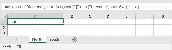
=MID(CELL("filename"),FIND("]",CELL("filename"))+1,255)

This formula works similarly to the RIGHT formula, where it first finds the position of the square bracket (using the FIND function).

It then uses the MID function to extract everything after the square bracket.

Fetching Sheet Name and Adding Text to it

If you’re building a dashboard, you may want to not just get the name of the worksheet, but also append a text before or after it.

For example, if you have a sheet name 2021, you may want to get the result as ‘Summary of 2021’ (and not just the sheet name).

This can easily be done by combining the formula we saw above with the text we want before it using the ampersand operator.

Below is the formula that will add the text ‘Summary of ‘ before the sheet name:

="Summary of "&RIGHT(CELL("filename"),LEN(CELL("filename"))-FIND("]",CELL("filename")))

Formula to append text before the sheet name in Excel

The ampersand operator (&) simply combines the text before the formula with the result of the formula. You can also use the CONCAT or CONCATENATE function instead of an ampersand.

Similarly, if you want to add any text after the formula, you can use the same ampersand logic (i.e., have the ampersand after the formula followed by the text that you want to append).

So these are two simple formulas that you can use to get the sheet name in Excel.

I hope you found this tutorial useful.

Other Excel tutorials you may also like:

How to Rename a Sheet in Excel (4 Easy Ways + Shortcut)
How to Insert New Worksheet in Excel (Easy Shortcuts)
How to Unhide Sheets in Excel (All In One Go)
How to Sort Worksheets in Excel using VBA (alphabetically)
Combine Data From Multiple Worksheets into a Single Worksheet in Excel
How to Compare Two Excel Sheets
How to Group Worksheets in Excel

Источник

In this example, the goal is to return the name of the current worksheet (i.e. tab) in the current workbook with a formula. This is a simple problem in the latest version of Excel, which provides the TEXTAFTER function. In older versions of Excel, you can use an alternative formula based on the MID and FIND functions. Both formula options rely on the CELL function to get a full path to the current workbook. Read below for a full explanation.

Workbook path

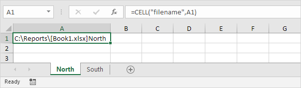
The first step in this problem is to get the workbook path, which includes the workbook and worksheet name. This can be done with the CELL function like this:

CELL("filename",A1)

With the info_type argument set to «filename», and reference set to cell A1 in the current worksheet, the result from CELL is a full path as a text string like this:

"C:pathtofolder[workbook.xlsx]sheetname"

Notice the sheet name begins after the closing square bracket («]»). The problem now becomes how to extract the sheet name from the path? The best way to do this depends on your Excel version. Use the TEXTAFTER function if available. Otherwise, use the MID and FIND functions as explained below.

TEXTAFTER function

In Excel 365, the easiest option is to use the TEXTAFTER function with the CELL function like this:

=TEXTAFTER(CELL("filename",A1),"]")

The CELL function returns the full path to the current workbook as explained above, and this text string is delivered to TEXTAFTER as the text argument. Delimiter is set to «]» in order to retrieve only text that occurs after the closing square bracket («]»). In the example shown, the final result is «September» the name of the current worksheet in the workbook shown.

MID + FIND function

In older versions of Excel that do not offer the TEXTAFTER function, you can use the MID function with the FIND function to extract the sheet name:

=MID(CELL("filename",A1),FIND("]",CELL("filename",A1))+1,255)

The core of this formula is the MID function, which is used to extract text starting at a specific position in a text string. Working from the inside out, the first CELL function returns the full path to the current workbook to the MID function as the text argument:

CELL("filename",A1) // get full path

We then need to tell MID where to start extracting text. To do this, we use the FIND function with a second call to the CELL function to locate the «]» character. We want MID to start extracting text after the «]» character, so we use the FIND function to get the position, then add 1:

FIND("]",CELL("filename",A1))+1 // get start number

The result from the above snippet is returned to the MID function as start_num. For the num_chars argument, we hard-code the number 255*. The MID function doesn’t care if the number of characters requested is larger than the length of the remaining text, it simply extracts all remaining text. The final result is «September» the name of the current worksheet in the workbook shown.

*Note: In Excel user interface, you can’t name a worksheet longer than 31 characters, but the file format itself permits worksheet names up to 255 characters, so this ensures the entire name is retrieved.

Источник

Содержание

Get Sheet Name
Insert Sheet Name In Cell: Easy! 3 Methods to Return the Worksheet Name
Method 1: Insert the sheet name using built-in Excel functions
How to Get the Current Sheet Name
Example
Generic Formula
What It Does
How It Works
Excel Formula – Get Worksheet Name
Get Worksheet Name – Excel Formula
The CELL Function:
The FIND Function:
The MID Function
Get Sheet Name in VBA
Examples of using the SHEET and SHEETS functions in Excel formulas
SHEET and SHEETS functions in Excel: description of arguments and syntax
How to get sheet name by formula in Excel
Examples of using the SHEET function and SHEETS
Processing information about the sheets of the book on the formula Excel

Get Sheet Name

To return the sheet name in a cell, use CELL, FIND and MID in Excel. There’s no built-in function in Excel that can get the sheet name.

1. The CELL function below returns the complete path, workbook name and current worksheet name.

Note: instead of using A1, you can refer to any cell on the first worksheet to get the name of this worksheet.

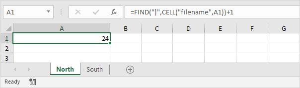
2. Use the FIND function to find the position of the right bracket. Add 1 to return the start position of the sheet name.

3. To extract a substring, starting in the middle of a string, use the MID function. First argument (formula from step 1). Second argument (formula from step 2). Third argument (31).

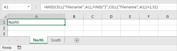
Explanation: the MID function shown above starts at position 24 and extracts 31 characters (maximum length of a worksheet name).

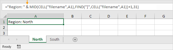
4. You may want to add text to the name of the sheet. Simply use the ampersand (&) operator as shown below.

5. To get the name of the second worksheet, simply refer to any cell on the second worksheet.

Pro tip: use Excel VBA to display the sheet names of all Excel files in a directory. You can find detailed instructions here.

Источник

Insert Sheet Name In Cell: Easy! 3 Methods to Return the Worksheet Name

Often, you need to insert and work with the sheet name in an Excel sheet, for example if you are working with the ‘INDIRECT’-formula. Or, if you want to dynamically change headlines depending on the sheet name. If you don’t want to type the sheet name manually – which is very unstable – there are three ways to get a sheet name

Before we start: If you just have to insert the sheet name for a small amount of worksheets, please consider doing it manually. It usually is the fastest way.

Method 1: Insert the sheet name using built-in Excel functions

The easiest way is to copy the following function and paste it into your Excel cell:

This formula obtains the filename “=CELL(“filename”,A1)” and separates it after the character “]”. If you want to get the name of another Excel sheet, you have to change the cell reference from “A1” to any cell of the other worksheet. And depending on your version and language of Excel, you might have to translate the function names and maybe replace “,” by “;”.

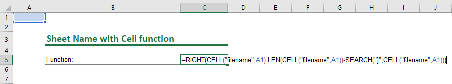Insert a sheet name with the cell function.

The big advantages of this method is that it doesn’t require any programming in VBA or a third-party Excel add-in.

On the downside, please note the following comments:

If you open a new file and paste this function, it won’t work before saving it.
The cell function is volatile. That means, it always calculates no matter if you’ve changed anything. This is a disadvantage for large Excel files where the performance of calculation is crucial.
Also, the cell function doesn’t translate to other languages. If your Excel is set to German, Spanish etc., you have to replace the “filename” part with the respective word in your language.

Do you want to boost your productivity in Excel?

Get the Professor Excel ribbon!

Add more than 120 great features to Excel!

Источник

How to Get the Current Sheet Name

Example

Generic Formula

filename – This is a system defined input for the CELL function.

What It Does

This formula will return the sheet name of the current sheet.

How It Works

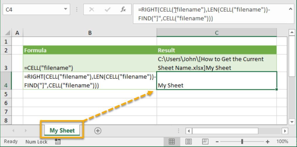
CELL(“filename”) will return the full file path of the current workbook (let’s call this the FilePath) which includes the folder path, workbook name and the current sheet name. In our example FilePath is C:UsersJohn[How to Get the Current Sheet Name.xlsx]My Sheet.

FIND(“]”,FilePath) will return the location of the “]” character before the sheet name (let’s call this the Location). In our example FIND(“]”,FilePath) returns the value 132 since “]” is the 132nd character in the FilePath text string.

LEN(FilePath) will return the total character length of the FilePath text string (let’s call this the TotalLength). In our example LEN(FilePath) returns the value 140 since there are 140 characters in the text string.

We can now get the length of the sheet name by subtracting TotalLength-Location. In our example the sheet name length is 140-132=8 characters.

RIGHT(FilePath,TotalLength-Location) will then return the right most 8 characters of the FilePath, which gives us the sheet name. In our example this is My Sheet.

Источник

Excel Formula – Get Worksheet Name

Download the example workbook

Use this Excel formula to get the worksheet name

Get Worksheet Name – Excel Formula

To calculate the worksheet name in one Excel Formula, use the following formula:

Notice in the image above this formula returns sheet names GetWorksheetName and Sheet3.

This code may look intimidating at first, but it’s less confusing if you split it out into separate formulas:

Excel Functions – Worksheet Name

The CELL Function:

The Cell Function returns information about a cell. Use the criteria “filename” to return the file location, name, and current sheet.

The FIND Function:

The CELL Function returns [workbook.xlsx]sheet , but we only want the sheet name, so we need to extract it from the result. First though, we need to use the FIND Function to identify the location of the sheet name from the result.

The MID Function

Next, we will extract the desired text using the MID Function with the result of the FIND Function (+1) as the start_num.

Why did choose 999 for the num_characters input in the MID Function? 999 is a large number that will return all remaining characters. You could have chosen any other significantly large number instead.

Get Sheet Name in VBA

If you want to use VBA instead of an Excel Formula, you have many options. This is just one example:

Enter the current worksheet name in cell A1 using VBA.

Источник

Examples of using the SHEET and SHEETS functions in Excel formulas

SHEET function in Excel returns a numeric value corresponding to the sheet number referenced by the link passed to the function as a parameter.

SHEET and SHEETS functions in Excel: description of arguments and syntax

SHEETS function in Excel returns a numeric value that corresponds to the number of sheets referenced.

Both functions are useful for use in documents containing a large number of sheets.
A sheet in Excel is a table of all the cells that are displayed on the screen and are outside of it (a total of 1,048,576 rows and 16,384 columns). When sending a sheet to print, it can be divided into several pages. Therefore, the terms “sheet” and “page” should not be confused.
The number of sheets in the book is limited only by the amount of PC RAM.

Function has only 1 argument in its syntax and is optional for: =SHEET( value ).

value is an optional function argument that contains text data with the name of the sheet or a link for which you want to set the sheet number. If this parameter is not specified, the function will return the number of the sheet in one of the cells of which it was written.

When the sheet works, all sheets that are visible, hidden and very hidden are taken into account. Exceptions are dialogs, macros, and diagrams.
If the function argument is a text value that does not match the name of any of the sheets contained in the book, the error #NA will be returned.
If an invalid value was passed as an argument to the function, the result of its calculation will be the error #REF!.
Within the object model (the hierarchy of objects in VBA, in which Application is the main object and Workbook, WorkSheet, etc., are child objects), the SHEET function is not available because it contains a similar function.

The function has the following syntax: =SHEETS( reference ).

reference — an object of reference type for which you want to determine the number of sheets. This argument is optional. If this parameter is not specified, the function will return the number of sheets contained in the book where it was written.

This function counts the number of all hidden, very hidden and visible sheets, with the exception of charts, macros and dialogs.
If an invalid reference was passed as a parameter, the result of the calculation is the error code #REF!.
This function is not available in the object model due to the presence of a similar function there.

How to get sheet name by formula in Excel

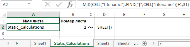
Example 1. In carrying out the calculated work the student used the Excel program, in which he created a book of several sheets. For his own convenience, the student decided to display in the cells A2 and B2 of each sheet data on the name of the sheet and its serial number, respectively. For this, he used the following formulas:

Description of arguments for the MID function:

=CELL(«filename») is a function that returns text in which the MID function searches for a specified number of characters. In this case, the value “C:UserssoulpDesktop[Workbook.xlsx] Static_Calculations” will return, where after the “]” symbol is the required text — the name.
=FIND(«]»,CELL(«filename»))+1 is a function that returns the position number of the character «]», one is added so that the MID function does not take into account the character].
31 — the maximum number of characters in the name.

=SHEET() — this function without parameter returns the number of the current sheet. As a result of its calculation, we get the number of sheets in the current book.

Examples of using the SHEET function and SHEETS

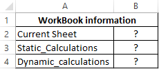
Example 2. The Excel workbook contains several sheets. It is necessary:

Return the current sheet number.
Return the sheet number with the name «Static_calculations».
Return the number of the sheet «Dynamic_calculations», if its cell A3 contains the value 0.

Enter the data in the table:

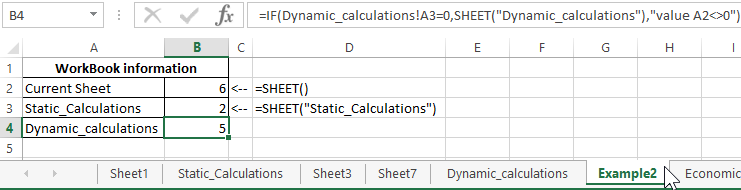
Next, we write the formulas for all 4 conditions:

For condition # 1, use the following formula: =SHEET()
For condition # 2, enter the formula: =SHEET(«Static_calculations»)
For condition number 3 we write the formula:

0″)’ >

The IF function checks whether the value stored in the A3 cell of the Dynamic_ calculations is equal to zero or null.

As a result, we get:

Processing information about the sheets of the book on the formula Excel

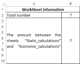
Example 3. To determine the contains several sheets. It is necessary to determine the total number of sheets, as well as the number contained between the “Static_calculations” and “Economic_calculations”.

The source table is:

The total number of sheets is calculated by the formula:

To determine the number contained between these two sheets, we write the formula:

Static_calculations: Economic_calculations!A2 — A reference to cell A2 of the range of sheets between «Static_calculations» and «Economic_calculations» including these sheets.
To get the desired value, 2 was subtracted.

As a result, we get the following:

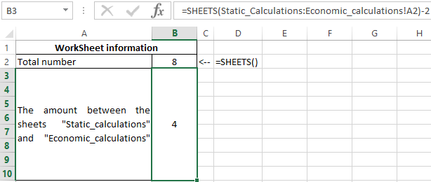
The formula displays detailed information on the data on the sheets in a certain range of their location in the Excel workbook.

Источник

Home / Excel Formulas / How to Get Sheet Name in Excel

In Excel, there is no direct function to get the sheet name of the active sheet.

Now the solution to this problem is to create a formula using multiple functions or to use a custom function created using the VBA.

In this tutorial, you will learn both methods with examples.

Use a Formula to Get the Worksheet Name

To create a formula to get the worksheet name we need to use CELLS, FIND, and MID function. Following is the function where you can get the sheet name.

=MID(CELL("filename"),FIND("]",CELL("filename"))+1,LEN(CELL("filename")))

You enter the above formula in any of the cells in the worksheet for which you want to have the sheet name. Now let’s understand this formula, and to understand this we need to break it up into four parts.

In the first part, we have a CELL function that returns the address of the workbook along with the current sheet’s name.

And, following is the address that we got from the cell function. Here you can see you have the sheet name at the end of the address, and you need to get the sheet name from it.

Now in the second part, we have the FIND function that uses the cell function to get the address and find the position of the character that you have exactly one position ahead of the sheet name.

And once you get the position number of “]”, you need to add 1 into it to get the position of the first character of the sheet name.

Now in the third part, you have the LEN and CELL functions to count of the characters in the entire path.

Now at this point, we have the address path, the position of the first character of the sheet name, and the count characters that we have in the address path.

And in the fourth part, by using the MID function you have got the sheet name in the result.

Create a User-Defined Function to Get Sheet Name

Getting a sheet name by a UDF is the easiest way. You don’t need to create a complex formula, but a simple code like the following.

Function mySheetName()
mySheetName = ActiveSheet.Name
End Function

Now let’s learn how we can use this code to extract the current worksheet’s name in a cell. Use the following steps:

First, go to the Developer tab and click on Visual Basic.
Now in the Visual Basic Editor, go to the Insert option and click on the Module to Insert a Module.
After that, go to the code window and paste the above code there.
In the end, close the visual basic editor and come back to the worksheet.

Now, select any of the cells in the worksheet for which you want to get the name and enter the following function there.

You can learn more about creating a custom function from this tutorial.

Источник

I have searched the excel function documentation and general MSDN search but have been unable to find a way to return the sheet name without VBA.

Is there a way to get the sheet name in an excel formula without needing to resort to VBA?

pnuts

58k11 gold badges85 silver badges137 bronze badges

asked Feb 1, 2015 at 17:27

Not very good with excel, but I found these here

=MID(CELL("filename",A1),FIND("]",CELL("filename",A1))+1,256)

and A1 can be any non-error cell in the sheet.
For the full path and name of the sheet, use

=CELL("filename",A1)

answered Feb 1, 2015 at 17:31

TravisTravis

1,2641 gold badge16 silver badges33 bronze badges

Here’s a reasonably short one that has a couple added benefits:

Does a reverse lookup (most other answers go wrong direction) by using the often ignored REPT function.
A1 seems like a poor choice as there’s a considerably higher chance it errors compared to… $FZZ$999999.
Don’t forget to absolute. Copying and pasting some of the other examples could error due to referential changes.

The ? is intentional as that shouldn’t be in the file path.

=SUBSTITUTE(RIGHT(SUBSTITUTE(CELL("Filename",$FZZ$999999), 
"]",REPT("?", 999)), 999),"?","")

answered Jun 20, 2019 at 0:38

pgSystemTesterpgSystemTester

8,7802 gold badges22 silver badges49 bronze badges

The below will isolate the sheet name:

=RIGHT(CELL("filename"),LEN(CELL("filename"))-FIND("]",CELL("filename")))

eli-k

10.7k11 gold badges43 silver badges44 bronze badges

answered Aug 8, 2016 at 3:52

For recent versions of Excel, the formula syntax is:

=MID(CELL("filename";A1);FIND("]";CELL("filename";A1))+1;255)

Wizhi

6,3684 gold badges24 silver badges47 bronze badges

answered Oct 17, 2018 at 10:59

OrbitOrbit

2121 silver badge7 bronze badges

None of the formulas given in other answers supports the case if there is character ] in filepath.

The formula below is more complex, but it can handle such cases properly:

 =MID(CELL("filename",A1),FIND("]",CELL("filename",A1),FIND("?",SUBSTITUTE(CELL("filename",A1),"","?",LEN(CELL("filename",A1))-LEN(SUBSTITUTE(CELL("filename",A1),"","")))))+1,LEN(CELL("filename",A1)))

answered Apr 19, 2019 at 1:47

mielkmielk

3,88012 silver badges19 bronze badges

I had a module already open so I made a custom function:

Public Function Sheetname (ByRef acell as Range) as string
Sheetname = acell.Parent.Name 
End Function

eli-k

10.7k11 gold badges43 silver badges44 bronze badges

answered Dec 21, 2017 at 15:00

Had a square bracket ‘]’ in the file name, so needed to modify the above formula as per the following to find the last occurrence of the square bracket.
Verified that this works for 0,1 or more square brackets in the file name / path.

=RIGHT(CELL("filename"),LEN(CELL("filename")) - FIND("]]]",SUBSTITUTE(CELL("filename"),"]","]]]",LEN(CELL("filename"))-LEN(SUBSTITUTE(CELL("filename"),"]","")))))

Replaces all square brackets using the substitute function, then compares the length of the result with the length of the file name to identify the number of square brackets in the file name.
Uses the number of occurrences of square brackets to substitute the last square bracket with 3 sequential square brackets ‘]]]’
Uses the Find function to identify the location of the 3 square brackets in the string
Subtracts the location of the 3 square brackets from the length of the full path
Uses the result to get the right most characters (being the sheet name)

Previous comment above about saving the workbook first is also a key, as you’ll otherwise receive the #Value! result.

answered Jun 14, 2019 at 2:27

JokeyJokey

313 bronze badges

The below works for me and is simpler (to me at least) than other solutions, while still handling a square bracket in the file name:

=MID(CELL("filename", A1),6+SEARCH(".xlsx]",CELL("filename", A1)),32)

This assumes it is an «xlsx» file and that the filename will not contain «.xlsx]» in addition to the xlsx suffix, which in my case is an assumption that is safe enough to make.

If you wanted to handle both «.xlsx» and «.xls» file names, you could use:

=MID(SUBSTITUTE(CELL("filename", A1),".xls]",".xlsx]"),6+SEARCH(".xlsx]",SUBSTITUTE(CELL("filename", A1),".xls]",".xlsx]")),32)

answered Dec 26, 2020 at 21:19

mwagmwag

3,36929 silver badges36 bronze badges

I’m pretty sure you could have Googled this. I just did, and here is the very first thing that came up for me.

In Excel it is possible to use the CELL function/formula and the MID and FIND to return the name of an Excel Worksheet in a Workbook. The formula below shows us how;

=MID(CELL("filename",A1),FIND("]",CELL("filename",A1))+1,256)

Where A1 is any non error cell on the Worksheet. If you want the full path of the Excel Workbook, simply use;

=CELL("filename",A1)

The only catch is that you have to save the file for this to work!

answered Feb 8, 2017 at 21:42

ASHASH

20.2k18 gold badges80 silver badges183 bronze badges

Источник