
Excel for Microsoft 365 Excel for Microsoft 365 for Mac Excel for the web Excel 2021 Excel 2021 for Mac Excel 2019 Excel 2019 for Mac Excel 2016 Excel 2016 for Mac Excel 2013 Excel 2010 Excel 2007 Excel for Mac 2011 Excel Starter 2010 More…Less
Use Excel’s DATE function when you need to take three separate values and combine them to form a date.
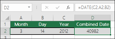
The DATE function returns the sequential serial number that represents a particular date.
Syntax: DATE(year,month,day)
The DATE function syntax has the following arguments:
-
Year Required. The value of the year argument can include one to four digits. Excel interprets the year argument according to the date system your computer is using. By default, Microsoft Excel for Windows uses the 1900 date system, which means the first date is January 1, 1900.
Tip: Use four digits for the year argument to prevent unwanted results. For example, «07» could mean «1907» or «2007.» Four digit years prevent confusion.
-
If year is between 0 (zero) and 1899 (inclusive), Excel adds that value to 1900 to calculate the year. For example, DATE(108,1,2) returns January 2, 2008 (1900+108).
-
If year is between 1900 and 9999 (inclusive), Excel uses that value as the year. For example, DATE(2008,1,2) returns January 2, 2008.
-
If year is less than 0 or is 10000 or greater, Excel returns the #NUM! error value.
-
-
Month Required. A positive or negative integer representing the month of the year from 1 to 12 (January to December).
-
If month is greater than 12, month adds that number of months to the first month in the year specified. For example, DATE(2008,14,2) returns the serial number representing February 2, 2009.
-
If month is less than 1, month subtracts the magnitude of that number of months, plus 1, from the first month in the year specified. For example, DATE(2008,-3,2) returns the serial number representing September 2, 2007.
-
-
Day Required. A positive or negative integer representing the day of the month from 1 to 31.
-
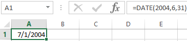
If day is greater than the number of days in the month specified, day adds that number of days to the first day in the month. For example, DATE(2008,1,35) returns the serial number representing February 4, 2008.
-
If day is less than 1, day subtracts the magnitude that number of days, plus one, from the first day of the month specified. For example, DATE(2008,1,-15) returns the serial number representing December 16, 2007.
-
Note: Excel stores dates as sequential serial numbers so that they can be used in calculations. January 1, 1900 is serial number 1, and January 1, 2008 is serial number 39448 because it is 39,447 days after January 1, 1900. You will need to change the number format (Format Cells) in order to display a proper date.
Syntax: DATE(year,month,day)
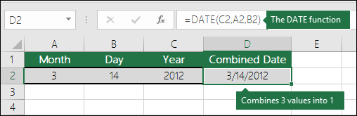
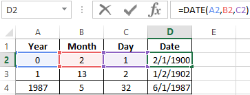
For example: =DATE(C2,A2,B2) combines the year from cell C2, the month from cell A2, and the day from cell B2 and puts them into one cell as a date. The example below shows the final result in cell D2.
Need to insert dates without a formula? No problem. You can insert the current date and time in a cell, or you can insert a date that gets updated. You can also fill data automatically in worksheet cells.
-
Right-click the cell(s) you want to change. On a Mac, Ctrl-click the cells.
-
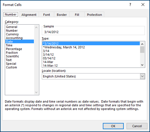
On the Home tab click Format > Format Cells or press Ctrl+1 (Command+1 on a Mac).
-
3. Choose the Locale (location) and Date format you want.
-
For more information on formatting dates, see Format a date the way you want.

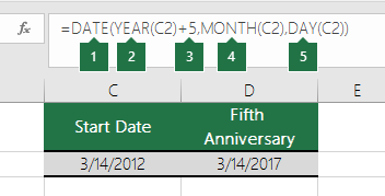
You can use the DATE function to create a date that is based on another cell’s date. For example, you can use the YEAR, MONTH, and DAY functions to create an anniversary date that’s based on another cell. Let’s say an employee’s first day at work is 10/1/2016; the DATE function can be used to establish his fifth year anniversary date:
-
The DATE function creates a date.
=DATE(YEAR(C2)+5,MONTH(C2),DAY(C2))
-
The YEAR function looks at cell C2 and extracts «2012».
-
Then, «+5» adds 5 years, and establishes «2017» as the anniversary year in cell D2.
-
The MONTH function extracts the «3» from C2. This establishes «3» as the month in cell D2.
-
The DAY function extracts «14» from C2. This establishes «14» as the day in cell D2.
If you open a file that came from another program, Excel will try to recognize dates within the data. But sometimes the dates aren’t recognizable. This is may be because the numbers don’t resemble a typical date, or because the data is formatted as text. If this is the case, you can use the DATE function to convert the information into dates. For example, in the following illustration, cell C2 contains a date that is in the format: YYYYMMDD. It is also formatted as text. To convert it into a date, the DATE function was used in conjunction with the LEFT, MID, and RIGHT functions.

-
The DATE function creates a date.
=DATE(LEFT(C2,4),MID(C2,5,2),RIGHT(C2,2))
-
The LEFT function looks at cell C2 and takes the first 4 characters from the left. This establishes “2014” as the year of the converted date in cell D2.
-
The MID function looks at cell C2. It starts at the 5th character, and then takes 2 characters to the right. This establishes “03” as the month of the converted date in cell D2. Because the formatting of D2 set to Date, the “0” isn’t included in the final result.
-
The RIGHT function looks at cell C2 and takes the first 2 characters starting from the very right and moving left. This establishes “14” as the day of the date in D2.
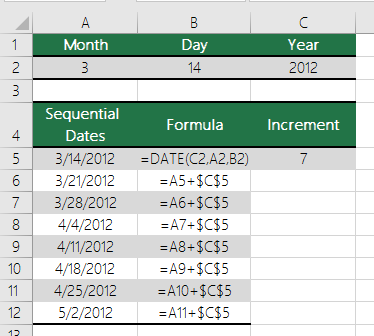
To increase or decrease a date by a certain number of days, simply add or subtract the number of days to the value or cell reference containing the date.
In the example below, cell A5 contains the date that we want to increase and decrease by 7 days (the value in C5).
See Also
Add or subtract dates
Insert the current date and time in a cell
Fill data automatically in worksheet cells
YEAR function
MONTH function
DAY function
TODAY function
DATEVALUE function
Date and time functions (reference)
All Excel functions (by category)
All Excel functions (alphabetical)
Need more help?
Want more options?
Explore subscription benefits, browse training courses, learn how to secure your device, and more.
Communities help you ask and answer questions, give feedback, and hear from experts with rich knowledge.
The current date and time is a very common piece of data needed in a lot of Excel solutions.
The great news is there a lot of ways to get this information into Excel.
In this post, we’re going to look at 5 ways to get either the current date or current time into our workbook.
Video Tutorial
Keyboard Shortcuts
Excel has two great keyboard shortcuts we can use to get either the date or time.
These are both quick and easy ways to enter the current date or time into our Excel workbooks.
The dates and times created will be current when they are entered, but they are static and won’t update.
Current Date Keyboard Shortcut
Pressing Ctrl + ; will enter the current date into the active cell.
This shortcut also works while in edit mode and will allow us to insert a hardcoded date into our formulas.
Current Time Keyboard Shortcut
Pressing Ctrl + Shift + ; will enter the current time into the active cell
This shortcut also works while in edit mode and will allow us to insert a hardcoded date into our formulas.
Functions
Excel has two functions that will give us the date and time.
These are volatile functions, which means any change in the Excel workbook will cause them to recalculate. We will also be able to force them to recalculate by pressing the F9 key.
This means the date and time will always update to the current date and time.
TODAY Function
= TODAY()This is a very simple function and has no arguments.
It will return the current date based on the user’s PC settings.
This means if we include this function in a workbook and send it to someone else in a different time zone, their results could be different.
NOW Function
= NOW()This is also a simple function with no arguments.
It will return the current date and time based on the user’s PC date and time setting.
Again, someone in a different time zone will get different results.
Power Query
In Power Query, we only have one function to get both the current date and current time. We can then use other commands to get either the date or time from the date-time.
We first need to add a new column for our date-time. Go to the Add Column tab and create a Custom Column.
= DateTime.LocalNow()In the Custom Column dialog box.
- Give the new column a name like Current DateTime.
- Enter the DateTime.LocalNow function in the formula section.
- Press the OK button.
Extract the Date
Now that we have our date-time column, we can extract the date from it.
We can select the date-time column ➜ go to the Add Column tab ➜ select the Date command ➜ then choose Date Only.
= Table.AddColumn(#"Added Custom", "Date", each DateTime.Date([Current DateTime]), type date)This will generate a new column containing only the current date. Power query will automatically generate the above M code with the DateTime.Date function to get only the date.
Extract the Time
We can also extract the time from our date-time column.
We can select the date-time column ➜ go to the Add Column tab ➜ select the Time command ➜ then choose Time Only.
= Table.AddColumn(#"Added Custom", "Time", each DateTime.Time([Current DateTime]), type time)This will generate a new column containing only the current time. Power query will automatically generate the above M code with the DateTime.Time function to get only the time.
Power Pivot
With power pivot, there are two ways to get the current date or time. We can create a calculated column or a measure.
To use power pivot, we need to add our data to the data model first.
- Select the data.
- Go to the Power Pivot tab.
- Choose the Add to Data Model command.
Power Pivot Calculated Column
A calculated column will perform the calculation for each row of data in our original data set. This means we can use the calculated column as a new field for our Rows or Columns area in our pivot tables.
= TODAY()= NOW()It turns out Power Pivot has the exact same TODAY and NOW functions as Excel!
We can then add a new calculated column inside the power pivot add in.
- Double click on the Add Column and give the new column a name. Then select any cell in the column and enter the TODAY function and press Enter.
- Go to the Home tab ➜ Change the Data Type to Date ➜ Change the Format to any of the date formats available.
We can do the exact same to add our NOW function to get the time and then format the column with a time format.
Power Pivot Measure
Another option with power pivot is to create a measure. Measures are calculations that aggregate to a single value and can be used in the Values area of a pivot table.
Again, we can use the same TODAY and NOW functions for our measures.
Add a new measure.
- Go to the Power Pivot tab.
- Select the Measures command.
- Select New Measure.
This will open up the Measure dialog box where we can define our measure calculation.
- Give the new measure a name.
- Add the TODAY or NOW function to the formula area.
- Select a Date Category.
- Select either a date or time format option.
- Press the OK button.
Now we can add our new measure into the Values area of our pivot table.
Power Automate
If you’re adding or updating data in Excel through some automated process via Power Automate, then you might want to add a timestamp indicating when the data was added or last updated.
We can definitely add the current date or time into Excel from Power Automate.
We will need to use an expression to get either the current date or time. Power Automate expressions for the current time will result in a time in UTC which will then need to be converted into the desired timezone.
= convertFromUtc(utcNow(),'Eastern Standard Time','yyyy-MM-dd')This expression will get the current date in the EST timezone. You can find a list of all the timezone’s here.
= convertFromUtc(utcNow(),'Eastern Standard Time','hh:mm:ss')This expression will get the current time in the EST timezone.
Conclusions
Like most things in Excel, there are many ways to get the current date and time in Excel.
Some are static like the keyboard shortcuts. They will never update after entering them, but this may be exactly what we need.
The other methods are dynamic but need to be recalculated or refreshed.
Do you have any other methods? Let me know in the comments!
About the Author
John is a Microsoft MVP and qualified actuary with over 15 years of experience. He has worked in a variety of industries, including insurance, ad tech, and most recently Power Platform consulting. He is a keen problem solver and has a passion for using technology to make businesses more efficient.
Sample Files
1. DATE Function
DATE function returns a valid date based on the day, month, and year you input. In simple words, you need to specify all the components of the date and it will create a date out of that.
Syntax
DATE(year,month,day)
Arguments
- year: A number to use as the year.
- month: A number to use as the month.
- day: A number to use as a day.
Example
In the below example, we have used cell references to specify the year, month, and day to create a date.

You can also insert arguments directly into the function to create a date as you can see in the below example.

And in the below example, we have used different types of arguments to see the result returned by the function.

2. DATEVALUE Function
DATEVALUE function returns a date after converting a text (which represents a date) into an actual date. In simple words, it converts a date into an actual date which is formatted as text.
Syntax
DATEVAUE(date_text)
Arguments
- date_text: The date which is stored as a text and you want to convert that text into an actual date.
Example
In the below example, we have inserted a date directly into the function by using double quotation marks. If you skip adding these quotation marks it will return a #NAME? error in the result.

In the below example, all the dates on the left side are in textual format.
- A simple textual date that we have converted into a valid date.
- A date with all three components (Year, Month, or Day) in numbers.
- If there is no year in the textual date, it will take the current year as the year.
- And if you have a month name is in alphabets and no year, it will take the current year as a year.
- If you don’t have the day in your textual date it will take 1 as the day number.

3. DAY Function
DAY function returns the day number from a valid date. As you know, in Excel, a date is a combination of day, month, and year, DAY function gets the day from the date and ignores the rest of the part.
Syntax
DAY(serial_number)
Arguments
- serial_number: A valid serial number of the date from which you want to extract the day number.
Example
In the below example, we have used the DAY to simply get the day from a date.

And in the below example, we have used DAY with TODAY to create a dynamic formula that returns the current day number and it will update every time you open your worksheet or when you recalculate your worksheet.

5. DAYS Function
DAYS function returns the difference between two dates. It takes a start date and an end date and then returns the difference between them in days. This function was introduced in Excel 2013 so not available in prior versions.
Syntax
DAYS(end_date,start_date)
Arguments
- start_date: It is a valid date from where you want to start the days’ calculation.
- end_date: It is a valid date from where you want to end the days’ calculation.
Example
In the below example, we have referred the cell A1 as the start date and B1 as the end date and we have 9 days in the result.
Note: You can also use the subtract operator to get the difference between two dates.

In the below example, we have directly inserted two dates into the function to get the difference between them.

6. EDATE Function
EDATE function returns a date after adding a specified number of months to it. In simple words, you can add (with a positive number) or subtract (with a negative number) months from a date.
Syntax
EDATE(start_date,months)
Arguments
- start_date: The date from which you want to start the calculation.
- months: The number of months to calculate the future or the past date.
Example
Here we have used EDATE with different types of arguments.
- In the first example, we have used 5 as a several months and it has added exactly 5 months on 1-Jan-2016 and returned 01-June-2016.
- In the second example, we have used -1 month and it has given 31-Dec-2016, a date which is exactly 1 month back from 31-Jan-2016.
- In the third example, we have inserted a date directly into the function.

7. EOMONTH Function
EOMONTH function returns the end of the month date which is the number of months in the future or the past. You can use a positive number for a future date and a negative number for the past month’s date.
Syntax
EOMONTH(start_date,months)
Arguments
- start_date: A valid date from where you want to start your calculation.
- months: The number of months you want to calculate before and after the start date.
Example
In the below example, we have used EOMONTH with different types of arguments:

- We have mentioned 01-Jan-2016 as the start date and 5 months for getting a future date. As June is exactly 5 months after January, it has returned 30-Jun-2016 in the result.
- As I have already mentioned, EOMMONTH is smart enough to evaluate the total number of days in a month.
- If you mention a negative number, it simply returns a past date which is the number of months back you have mentioned.
- In the fourth example, we have used a date that is in text format and it has returned the date without returning any errors.
8. MONTH Function
MONTH function returns the month number (ranging from 0 to 12) from a valid date. As you know, in Excel, a date is a combination of day, month, and year, MONTH gets the month from the date and ignores the rest of the part.
Syntax
MONTH(serial_number)
Arguments
- serial_number: A valid date from which you want to get the month number.
Example
In the below example, we have used a MONTH in three different ways:

- In the FIRST example, we have simply used date and it has returned the 5 in the result which is the month number of MAY.
- In the SECOND example, we have supplied the date directly in the function.
- In the THIRD example, we have used the TODAY function to get the current date and MONTH has returned the month number from it.
9. NETWORKDAYS Function
NETWORKDAYS function returns the count of days between the start date and end date. In simple words, with NETWORKDAYS you can calculate the difference between two dates, after excluding Saturdays and Sundays, and holidays (which you specify).
Syntax
NETWORKDAYS(start_date,end_date,holidays)
Arguments
- start_date: A valid date from where you want to start your calculation.
- end_date: A valid date up to which you want to calculate working days.
- [holidays]: A valid date that represents a holiday between the start date and end date. You can refer to a cell, range of cells, or an array containing dates.
Example
In the below example, we have specified 10-Jan-2015 as a start date and 20-Feb-2015 as an end date.

We have 41 days between these two dates, out of which 11 days are weekends. After deducting those 11 days it has returned 30 working days.
Now in the below example with the same start and end dates, we have specified a holiday and, after deducting 11 days of the weekend and 1 holiday it has returned 29 working days.

Again with the same start and end dates, we have used a range of three cells for holidays to deduct from the calculation and, after deducting 11 weekend days and 3 holidays which I have mentioned It has returned 27 working days.

10. NETWORKDAYS.INTL Function
NETWORKDAYS.INTL Function returns the count of days between the start date and end date. Unlike NETWORKDAYS, NETWORKDAYS.INTL lets you specify which days you want to exclude from the calculation.
Syntax
NETWORKDAYS.INTL(start_date,end_date,weekend,holidays)
Arguments
- start_date: A valid date from where you want to start your calculation.
- end_date: A valid date up to which you want to calculate working days.
- [weekend]: A number represents to exclude weekends from the calculation.
- [holidays]: A list of dates that represents the holidays you want to exclude from the calculation.
Example
In the below example, we have used 01-Jan-2015 as a start date and 20-Jan-2015 as an end date. And we have specified 1 to take Sunday – Saturday as the weekend. The function has returned 14 days after excluding 6 weekend days.

Below, we have used the same dates. And I have used 11 in for weekend days which means it will only consider Sunday as a weekend. Along with that, we have also used 10-Jan-2015 as a holiday.

We have 3 Sundays between both dates and a holiday. After excluding all these days the function has returned 16 days in the result. Here in the below example, we have used range to specify holidays. If you have more than one date for the holidays you can refer to an entire range.

Quick Tip: If you want to create a dynamic range for holidays, you can use a table for that. If you want to choose custom days to count as working days or weekends, you can use the below format in the weekend argument.

Here, 0 represents a working day and 1 represents a non-working day. And, seven numbers represent 7 days of the week.
11. TODAY Function
The TODAY function returns the current date and time as per the system’s date and time. The date and time returned by the NOW function update continuously whenever you update anything in the worksheet.
Syntax
TODAY()
Arguments
- In the TODAY function, there is no argument, all you need to do is enter it in the cell and hit enter, but be careful as TODAY is a volatile function which updates its value every time you update your worksheet calculations.
Example
In the below example, we have used TODAY with other functions to get the current month number, current year, and current day.

12. WEEKDAY Function
WEEKDAY function returns a day number (ranging from 0 to 7) of the week from a date. In simple words, the WEEKDAY function takes a date and returns the day number of that date’s day.
Syntax
WEEKDAY (serial_number, [return_type])
Arguments
- serial_number: A valid date from which you want to get the week number.
- [return_type]: A number that represents the day of the week to start the week.
Example
In the below example, we have used a WEEKDAY with TODAY to get a dynamic weekday. It will give you the weekday whenever the current date changes. You can use this method in your dashboards to trigger some values which need to change when weekday change.

In the below example, we have used WEEKDAY with IF to create a formula that first checks the weekday of date and return “Weekday” or “Weekend” basis on the value return from WEEKDAY.

13. WEEKNUM Function
WEEKNUM function returns the week number of a date. In simple words, WEEKNUM returns the week number of dates that you specify ranging from 1 to 54.
Syntax
WEEKNUM(serial_number,return_type)
Arguments
- serial_number: A date for which you want to get the week number.
- [return_type]: A number to specify the starting day of the first week of the year. You have two systems to specify the starting date of the week.
Example
In the below example, we have used TODAY with WEEKNUM to get the week number of the current date. It will update the week number automatically every time the date changes.

In the below example, we have added the text “Week-” with the week number for a meaningful result.

14. YEAR Function
YEAR Function returns the year number from a valid date. As you know, in Excel a date is a combination of day, month, and year, and the YEAR function gets the year from the date and ignores the rest of the part.
Syntax
YEAR(date)
Arguments
- date: A date from which you want to get the year.
Example
In the below example, we have used the year function to get the year number from the dates. You can use this function where you have dates in your data and you only need the year number.

And in the below example, we have used today function to get the year number from the current date. It will always update the year whenever you recalculate your worksheet.

The DATE function creates a date using individual year, month, and day arguments. Each argument is provided as a number, and the result is a serial number that represents a valid Excel date. Apply a date number format to display the output from the DATE function as a date.
In general, the DATE function is the safest way to create a date in an Excel formula, because year, month, and day values are numeric and unambiguous, in contrast to text representations of dates which can be misinterpreted.
Note: to move an existing date forward or backward in time, see the EDATE and EOMONTH.
Example #1 — hard-coded numbers
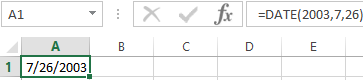
For example, you can use the DATE function to create the dates January 1, 1999, and June 1, 2010 with the following syntax:
=DATE(1999,1,1) // returns Jan 1, 1999
=DATE(2010,6,1) // returns Jun 1, 2010
Example #2 — cell reference
The DATE function is useful for assembling dates that need to change dynamically based on other inputs in a worksheet. For example, with 2018 in cell A1, the formula below returns the date April 15, 2018:
=DATE(A1,4,15) // Apr 15, 2018
If A1 is then changed to 2019, the DATE function will return a date for April 15, 2019.
Example #3 — with SUMIFS, COUNTIFS
The DATE function can be used to supply dates as inputs to other functions like SUMIFS or COUNTIFS, since you can easily assemble a date using year, month, and day values that come from a cell reference or formula result. For example, to count dates greater than January 1, 2019 in a worksheet where A1, B1, and C1 contain year, month, and day values (respectively), you can use a formula like this:
=COUNTIF(range,">"&DATE(A1,B1,C1))
The result of COUNTIF will update dynamically when A1, B1, or C1 are changed.
Example #4 — first day of current year
To return the first day of the current year, you can use the DATE function like this:
=DATE(YEAR(TODAY()),1,1) // first of year
This is an example of nesting. The TODAY function returns the current date to the YEAR function. The YEAR function extracts the year and returns the result to the DATE function as the year argument. The month and day arguments are hard-coded as 1. The result is the first day of the current year, a date like «January 1, 2021».
Note: the DATE function actually returns a serial number and not a formatted date. In Excel’s date system, dates are serial numbers. January 1, 1900 is number 1 and later dates are larger numbers. To display date values in a human-readable date format, apply the number format of your choice.
Notes
- The DATE function returns a serial number that corresponds to an Excel date.
- Excel dates begin in the year 1900. If year is between zero and 1900, Excel will add 1900.
- The DATE function accepts numeric input only and will return #VALUE if given text.
For work with dates in Excel, in the category «Date and time» is defined in the functions section. Let`s consider the most prevalent functions in this category.
How Excel Processes Time
The Excel program «perceives» the date and time as an ordinary number. The spreadsheet converts to such number, equating the day to unity. As a result, the time value represents a fraction of unity. For example, 12. 00 — is 0. 5.
The date value to the spreadsheet converts to a number which equal to the number of days from January 1, 1900 (so the developers decided) to the specified date. For example, when converting the date 13. 04. 1987, the number is 31880. That is, from 1. 01. 1900 passed 31. 880 days.
This principle underlies in the basis of the calculations of the time data. To find the number of days between two dates, it`s enough to take an earlier period from a later time one.
The example of DATE function
You need to describe of the date value with compiling it with individual elements of numbers.
There is the syntax: year; month, day.
All arguments are required. They can be specified by numbers or by reference to cells with the corresponding numeric data: for the year — from 1900 to 9999; for the month — from 1 to 12; for the day — from 1 to 31.
If you point a larger number for the «Day» argument (than the number of days in the pointed month), you receive the extra days, will be passed to the next month. For example, specifying 32 days for December, we will receive as a result on January 1.
The example of using the function:
Let’s set more days for June:
Examples of using the cell references as arguments:
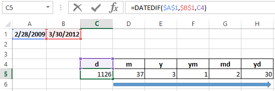
The DATEDIF function in Excel
It returns the difference between two dates.
The arguments:
- start date;
- final date;
- the code indicating to the units of counting (days, months, years, etc.).
The methods of measuring intervals between the given dates:
- to display the result in days — «d»;
- in months – «m»;
- in years – «y»;
- in months without years – «ym»;
- in days without months and years – «md»;
- in days without years – «yd».
In some versions of Excel, if you use the last two arguments («md», «yd»), the function may give an error. It is better to use to alternative formulas.
The examples of the operation the DATEDIF function:
In Excel 2007 version, this function is not in the directory, but it works. But you need to check the results are better, because there are flaws possible.
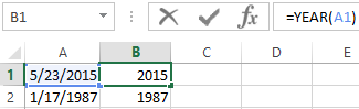
The YEAR function in Excel
It returns the year as an integer number (from 1900 to 9999), what corresponds to the specified date. There is only one argument must be entered in the structure of the function – is the date in a numerical format. The argument must be entered using the DATE function or represents to the result of evaluating other formulas.
The example of using the YEAR function:
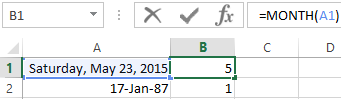
The MONTH function in Excel: the example
It returns the month as an integer number (from 1 to 12) for a date is specified in a numeric format. The argument – is the date of the month that you want to show in a numerical format. The dates in the text format this function does not handle correctly.
The examples of using the MONTH function:
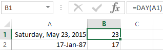
The examples of DAY, WEEKDAY and functions WEEKNUM in Excel
It returns the day as an integer number (from 1 to 31) for a date specified in a numeric format. The argument – it is the date of the day you want to find in a numerical format.
For returning of the weekday ordinal of the specified date, you can apply the function WEEKDAY:
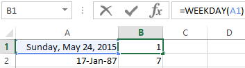
By default, the function considers Sunday the 1-st day of the week.
To display of the ordinal number of the week for the pointed date, you should use the WEEKNUM function:
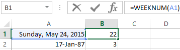
The date of 24. 05. 2015 is 22 week in a year. The week starts on Sunday (by default).
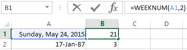
As the second argument the figure 2 is specified. Therefore, the formula considers that the week starts on Monday (the 2-d day of the week).
Download all examples functions for working with dates
For indicating of the current date, the function TODAY (no arguments) is used. To display the current time and date, the function NOW() is used.