
Microsoft Excel is a great tool, but sometimes the spreadsheet files we get to work with aren’t ideal. One example is a file with a data column, maybe a street address, that you’d really like to pull apart. In this tutorial, I’ll show how to extract text from a cell in Excel using some powerful, but simple text functions. (Includes practice workbook.)
What’s an Excel Substring?
Before we have Excel extract text from string, we need to define some things. Some programming languages have dedicated substring functions. Excel does something similar using Text functions. They have their own category.

When we speak of a substring, we mean a part or subset of the Excel cell’s content. For example, if the cell contained 1001 Drake Ave., any of these items could be a substring:
- 1001
- Drake Ave.
- 100
- rake
A Common Problem
Many membership databases or mailing lists are set up with defined fields for First Name, Last Name, Street, City, State, and Zip. This format works fine if you’re creating a mailing label as the post office relies on zip code sorting. And sometimes you can luck out and parse first and last names using Excel’s Convert Text to Columns Wizard.
But what if you need to do door-to-door canvassing to check on neighbors or to inform people about an upcoming ballot measure?
If you open this type of list in Excel and sort it on the Street column, you get a numerically sorted list. As you can see in the example below, the Drake Ave records are not together.
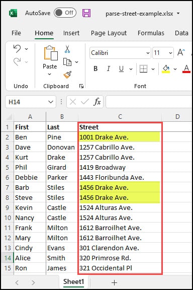
Ideally, you want to sort the list so the Drake Ave. entries are together. There are several ways to do this in Excel, but one way is to create two columns from the Street column.
The first column reflects the street number substring, and the second the street name substring. You can then resort the list based on the street name and street number.
Visually Building the Nested Formula
For the first example, we’ll nest some Excel functions such as LEFT and FIND. As we progress, we’ll add several sets of parentheses. By nested, I mean we’ll use one function (FIND) as an argument for another function such as LEFT or RIGHT.
Let’s start with =FIND(" ",C2). In plain text, our function syntax is asking Excel to look in reference cell C2 for a blank space which is represented by the ” “. In the picture below, I added a starting position of “1“, but this is an optional parameter and Excel starts at 1 by default. Excel found the blank space in position 5 which shows in cell D2.

To make the formula easier, I’ll remove the optional starting parameter of 1 since Excel starts there anyway.
Now, let’s add the LEFT function so that our formula reads =LEFT(C2,(FIND(" ",C2))). In this instance, we’re again using cell C2, but the LEFT function is going to grab the cell contents in C2 from position 1 to position 5 where the Excel FIND function found the blank space.

However, there is a minor issue. While you can’t see it, there is a trailing space in D2. Using the LEN function we can see cell D2 has 5 characters. You may remember this handy function from our tutorial on how to check character count in Excel.

The solution is to subtract 1 or use the TRIM function which I referenced in how to separate names in Excel. For simplicity, I’ll use the -1. While the visual results are the same, you can see the character count dropped by 1.

- Import your data into Microsoft Excel or use the sample spreadsheet in the Resources section.
- In cell D1, type Nbr.
- In cell E1, type Street Name
- In cell D2, type the following Excel formula
=LEFT(C2,(FIND(" ",C2)-1)) - Press Enter. The value 1001 should show in D2.
The next part involves copying this formula to the rest of the entries. However, we need to reference the correct street cell and not use C2 for the remaining rows.
- Click cell D2 to select the beginning of our range.
- Move your mouse to the lower right corner.

- Double-click the + cursor in the lower right. This will copy your formula down the column.
In column D, you should see the extracted street numbers.
We’ll now create a similar nested formula to capture the street address using the RIGHT function. This time, we will grab the contents to the right of the first space from the Street column.
- In cell E2, type the following formula
=RIGHT(C2,LEN(C2)-FIND(" ",C2)) - Press Enter. E2 should show as Drake Ave.
- Click cell E2 to select the beginning of our range.
- Move your mouse to the lower right corner.
- Double-click the + cursor in the lower right. This will copy your formula down the column.
Columns D and E should contain the parsed contents from your original street address.
Your spreadsheet should look similar to the one below.

Clean Up the Spreadsheet and Change Cell Format
The spreadsheet now has your split fields, but you should clean up the formulas. My suggestion would be to convert the LEFT and RIGHT formulas to their respective values. We did an earlier tutorial on how to copy formula values in Excel to values.
After you convert the Nbr column, you probably want to change the format type to a number.
- Click column D.
- Right-click and select Format cells...
- On the Format Cells dialog box, select Number.
- Set Decimal places to 0.
- Click OK.
Although our example extracted text from an Excel cell containing street information, you can use the same process to parse other entries. For example, Step 1 above is really parsing everything but the first word because it is searching for a blank space. You can alter the formula to find different values, such as a comma or an @ sign.
Excel Practice File
Hand-picked Excel Tutorials
Our Comment Policy.
We welcome your comments and questions about this lesson. We don’t welcome spam. Our readers get a lot of value out of the comments and answers on our lessons and spam hurts that experience. Our spam filter is pretty good at stopping bots from posting spam, and our admins are quick to delete spam that does get through. We know that bots don’t read messages like this, but there are people out there who manually post spam. I repeat — we delete all spam, and if we see repeated posts from a given IP address, we’ll block the IP address. So don’t waste your time, or ours. One other point to note — if you post a link in your comment, it will automatically be deleted.
Add a comment to this lesson
.
Comments on this lesson
Bringing only selected data forward
I have a job costing calculator and i only want to bring text forward to a front sheet in the workbook to summarize the selections. For example: the calculator lists several items offered, I want to bring only the items selected to a front page for a summary of the items selected to that specific job. So if there are 100 items that could be chosen, and only 5 are selected, I want to have a table that shows those 5 items only. AND the items are text not numerical value.
SO the job costing page may have : Window Removal and a cell to populate a number [number of windows to be removed] if that cell has a value greater than 0 i want the text «window removal» brought to another table for summary…I have tried IF functions and am not getting desired result…please help. Thanks
.
Extract number
I would like to extract the number out of column G (Description of goods) into column H (serial numbers) can you assist with a formula
.
Useful tips
Thanks 5 minutes were really 5 minutes and managed to extract data i wanted. Good work.
.
Extracting Numbers From a String
I am trying to separate the numbers from a string of text that contains numbers. The following is a sample string:
C4-14-3-6-21
I’d like to get the numbers into individual cells (except for the C4 part of the string which never changes). 14 is the year and will always be two digits. 3 will eventually become 2 digits long and then 3 and finally 4. The 6 will probably never be more than 2 digits long and the 21 can go 5 or 6 digits long. So far, I was able to create the following formulas that isolated the year (14) and the 3 (next number to the right):
=0+MID(A1,4,FIND(«-«,A1,4)-4)
=0+MID(A1,7,FIND(«-«,A1,7)-7)
It seems to work for the 14 and 3 slots. I haven’t been successful extracting the 6 and 21 (after testing different number of digits). Can you help me get these formulas right to extract all of the numbers?
.
LEFT
In the last exemple «=RIGHT(A1,LEN(A1)-FIND(«.»,A1))» how to do it to get just the names instead of the numbers? Because if you use «=LEFT(A1,LEN(A1)-FIND(«.»,A1))» it give all sting.
Thanks
.
Extract Text from a Cell in Excel
Hi there,
I am trying to extract the set of numbers before the first «~»
My attempt using Formula=RIGHT(A1,LEN(A1)-FIND(«.»,A1)) returned a «0»
3932730~20~17074~S2930248~1~14~S~A-07-02-08~~1
517398~1~17074~S2930248~1~27~S~A-04-07-02
345219~1~17074~S2930248~1~5~S~A-03-01-04
239068~1~17074~S2930248~1~33~S~A-06-05-03
3935400~1~17074~S2930248~1~17~S~A-07-02-03
345219~20~17074~S2930248~1~5~S~A-03-01-04~~1
1742393~1~17074~S2930248~1~36~S~B-16-04-07
Can you please help with this? Kind regards,
Brian
.
Brian,
Brian,
Try using =Left(A1,FIND(«~»,A1)-1)
.
Use Find/Replace
I Know I am very late, but just use replace option with text to find as «~*» and replace with null «»
.
Hello I’m trying to separate
Hello I’m trying to separate specific parts of text from a set of addresses. For example:
800 E DIMOND BLVD STE 127
800 E DIMOND BLVD SUITE 127
320 W 5TH AVE
3048 MOUNTAIN VIEW DR BLDG 119
2120 US HIGHWAY 92 W
On this text I would like to separate the last two parts which are «ste» and «127» to a separate column, the thing is that some addresses don’t have «ste» instead they have «suite» » building», etc. Is there any way that would be possible?
.
Moe,
Moe,
I’m sure it is possible, but I’m not the expert that could tell you how to do it. I’m sorry. I posted my original question to extract a single number from a string of numbers separated by hyphens. Try posting your question as a new string. Good luck.
Regards,
Lubo
.
leaving instead of extracting last octet
I am trying to get only the last octet of an ip address that is in a cell. Instead of using text to columns is there a way to leave only the last octet?
.
no result from Mid command
Col A B C D E F G
Invoice Status Cd State Acct Company Code Invoice Number Invoice Date Contract Number ARN
CO TX S580 65336 1/13/2014 NREC_TX_185584_CTL =MID(F2,9,6)
Using the MID formula listed under the ARN field, I am getting no result whatsoever. Excel 2007 file type .xlxs. What I want is in the ARN column G the number 185584.
.
minor update
dang, it didn’t save my spaces betweent the column numbers. Col F has the Contract Number.
.
extract lot number
6006 — Silicone Tip Capsule Polisher 23gX7mm bend Lot#: 04146016 Loc.: 5
5003AF — Irrigating Cystotome 25gX16mm (5/8″) formed Lot#: 12146050 Loc.: 84-86
Retrobulbar Needle 23gX1 1/2″ (Atkinson Point) Lot#: 01156001
3 different rows, what I need: «Lot#: xxxxxxxx» or just the 5th digit in the lot #, in these rows it would be «6» (if you look at my attachment, Column L & M work for must but since the location [Loc] has a different number of digits, notice cell M3 cuts off some of the Lot #.
TYIA
.
Extracting three different parts of a cell
I need to extract three different parts in the below string of text. I need to extract flavors loved to return «Fruits, Fruits & Cream, Dessert» (it can include quotations in the text. Flavors hated «Tobacco, discovery», then Nicotine level «Low (6mg)
{«flavors_loved»:[«Fruits»,»Fruits & Cream»,»Dessert»],»flavors_hated»:»Tobacco»,»discovery»:»Expand Range»,»nicotine_level»:[«Low (6mg)»]}
.
How to extract numbers within square brackets
Hi,
I have a spreadsheet contains several thousand of records.
These records (column A) contains text strings at and numbers within a square brackets at many various lengths.
What I would like to achieve is how extract just the numbers within the square brackets of column A into a new column. Examples of records as follow;
«Bangalore Street» Beams Road [4069]
«Clifton Hill» O/B Ipswich Road FS Beaudesert Rd [10386]
«HOMEBASE» [3368]
Could someone assist me.
Thanks in advance
.
This is a bit messy, but it
This is a bit messy, but it works.
=mid(A1,find(«[«,A1)+1,find(«]»,A1)-find(«[«,A1)-1)
.
Thanks so much Cionn.
Thanks so much Cionn.
I’ve performed search & replace the open square bracket replaced with symbol then did find formular similar to yours and it works the same way as yours. Thanks for responding to my call for help. Cheers
.
Sorting problem
Below is a sample cell value within my spreadsheet (it’s voting history- general election, primary election). I want to be able to sort using this column. The sorting would be, for example, all persons with a GE14 and a GE12 and a PE11. And various combinations like that. How could I accomplish that?
GE14GE13PE13GE12GE08GE04GE01GE00GE97
.
More information please …
Hi Matt
Can you be more specific about what you want to achieve? You say you want to sort, but I don’t have enough information to decide where, say, someone with GE14, G13 and PE11 might be ranked compared to someone with GE14, GE13 but not PE11.
Also, can you provide a couple of additional samples, and decode the formula? For example, it looks like this is a person who voted in the General Election in 2014, 2013, 2012, 2008, 2004, 2001, 2000 and 1997, and in a Primary Election in 2013. What I can’t tell is whether these are the only years in which elections were held, or if there was, say, a GE every year, but this person didn’t vote in every one of them.
Thanks.
David
.
Hi David. Thanks for the
Hi David. Thanks for the help. The value in this column is that person’s individual voting history. I’m not interested in ranking them. I only want to parcel out those people who, say, voted in GE14, GE12, and GE10. If all three of those values don’t appear in this cell, then (for present sorting purposes) I’m not interested in that person. So I’m wondering what formula I would use. Some sort of if(and(search…As you’ve probably guessed, I’m a novice exceller. Tks for any guidance you can provide.
.
Finding numbers
Hi,
I am a stock markets professional and have an excel file with hundreds of records in the following sample formats:
NIFTY JUN 8500 CE
BANKNIFTY JUL 18800 PE
STAR AUG 1300 CE
INDUSINDBK JAN 900 CE
JPASSOCIAT AUG 10 PE
What I want to do is just extract the numbers out of these cells and use it in a separate formula. I would be grateful if somebody could help me with this.
Regards,
Vikas.
.
Extracting $ amount from a cell
Hello —
Here is an example where all I want to extract is the $4,532.50. I have several like this but not one is the same. I am just looking in that cell for the actual dollar amount and that is it. Is there a formula for that? And it can be in anywhere from $x.xx to $xxx,xxx.xx. Thanks for your assistance.
Archive Hans Wegner Table (DS) AX 2364 $4,532.50 080315 #202061,86 3520
.
Pulling text from the end of a string to a new column
Pulling text from the end of a string to a new column, with different length prefixes. I really need some help here 
I need to get the size indicator of the end of the Sku into the next column
The M, XL, L and S
How can I do this because they are different lengths?
.
This formula is almost what I need to do.
Hello,
This formula is what I need, but I need to see another step. In my case I do have » : » and I need to grab everything as the last » : «
Example:
MY Part number: Susp IP:Torsion bars:911:1-SAW911F19
I need to grab the last part of the number just this part 1-SAW911F19
This formula almost gets me what I need =RIGHT(A1,LEN(A1)-FIND(«:»,A1)) but it get me everything after the first » : «
Thank you for your help.
VH
.
Very percise and satisfying
Very percise and satisfying answer. Thank you so much, you are very helpful.
.
Same Problem here
Did you solve your problem? Mine is very similar.
rumo-log-RUMO3
bmfbovespa-BVMF3
vale-VALE5
itausa-ITSA4
banco-do-brasil-BBAS3
itau-unibanco-ITUB4
guarapes-GUAR4
braskem-BRKM5
estacio-participacoes-ESTC3
br-malls-par-BRML3
brasilagro-AGRO3
cosan-ltd-CZLT33
unicasa-UCAS3
grendene-GRND3
alupar-ALUP11
fii-cshg-jhsf-HGJH11
fii-bc-fund-BRCR11
portobello-PTBL3
mills-MILS3
cielo-CIEL3
I’m trying to get only the last caps words. This formula =RIGHT(B3;LEN(B3)-FIND(«-«;B3)) works great with data with only 2 words, but the rest bring me stuff that I dont need
.
Found it
This worked for me! =TRIM(RIGHT(SUBSTITUTE(E2,»-«,REPT(» «,100)),100))
Hope it works for you too!
.
pulling text of different lengths
I am trying to pull the model of a product (text and numerical) from the beginning of each cell into another column for total product model analysis. Some models have one word, some have 3-4 words plus a number.
example:
Big River P 700c, 555, 0
Spy Hill 7.3 P 27.5, L3, 0
Glass Creek Pro Carbon Q, 29, 0
I would like to extract:
Big River
Spy Hill 7.3
Glass Creek Pro Carbon
See attached for actual data
.
Extracting
ip address 10.10.10.10
ip address 10.10.10.11
ip address 10.10.10.12
.
.
How can we extract only: 10.10.10.10 and 10.10.10.11 and so on?
.
string with unequal characters with 2 delimiters
My data is of different lengths, and the only constant is that the part I want to remove is always the last 11 characters. Alternatively, the data I want to retrieve is up to but not including the second underscore: Here is a sample:
R5510BU010_MAIN_926030_PDF
R5510BU010_MAIN_926028_PDF
R5510BU021_ALL_925732_PDF
R5510BU021_REGULAR_926026_PDF
R5510BU010_MAIN_925736_PDF
R5510BU021_REGULAR_925734_PDF
R5510BU010_MAIN_925738_PDF
R5510BU021_ALL_926024_PDF
R5510BU021_REGULAR_925468_PDF
R5510BU010_MAIN_925470_PDF
R5510BU010_MAIN_925472_PDF
What I am trying to do is retrieve everything up to but not including the second underscore. I can’t use left because the fields are unequal lengths, and when I use right, it returns the stuff I’m trying to remove.
Is there a better way?
Thanks
.
Addendum to above question
Sorry, I forgot to add:
I tried this formula: =LEFT(G2,LEN(G2)-FIND(«_»,G2)) and it returned:
R5510BU010_MAIN
R5510BU010_MAIN
R5510BU021_ALL
R5510BU021_REGULAR
R5510BU010_MAIN
R5510BU021_REGULAR
R5510BU010_MAIN
R5510BU021_ALL
R5510BU021_REGULAR
R5510BU010_MAIN
R5510BU010_MAIN
This looks great, but when I copied to down to the rest of the cells I got this:
R09801_ZJDE0002_926264_PDF returned R09801_ZJDE0002_926
R09801_ZJDE0002_925803_PDF returned R09801_ZJDE0002_925
R09801_ZJDE0002_925801_PDF returned R09801_ZJDE0002_925
R09801_ZJDE0002_925805_PDF returned R09801_ZJDE0002_925
R09801_ZJDE0002_925807_PDF returned R09801_ZJDE0002_925
R09801_ZJDE0002_925809_PDF returned R09801_ZJDE0002_925
R09801_ZJDE0002_925811_PDF returned R09801_ZJDE0002_925
R09801_ZJDE0002_926290_PDF returned R09801_ZJDE0002_926
Why did it seem to understand in the first selection but not the second?
Thanks
.
Ease of access to specific issues in 5 minute lessons
Thank you very much for putting up 5 minute lessons. They work better than excel help menu and the explanations are far more comprehensive & useful. I use 5 minute lesson as my excel help menu.
.
Extract text from a cell
I have a situation where I need to extract some or all of the DATA in a cell.
I am an options trader and at the end of the day i would like to know the underlying stock symbol for the option which will help easily filter and sort the trades.
stock symbols normally range between 1 and 4 letters
GDX
GDX 160708P28
GDX 160708P28
BBRY 160916C9
SLV 160805C19.5
SLV
=LEFT(B11,FIND(» «,B11))
This works fine for the option chain, but if its just the stock»SLV» it returns an error
The values im looking for are listed below
GDX
GDX
GDX
BBRY
SLV
SLV
Thanks for your help
.
Extracting Multiple info from a string of text
The below contains info found in a cell separated by commas. I’d to separate each of the info grouped by commas and put into different cells. At the moment I can only extract only the first set «PKL70080P» using =LEFT(A65,FIND(«,»,A65)-1). The rest I’m not sure how to do that.
PKL70080P,»Tbitha 318* x .02 LB OPT»,TPLin,5/12/2011,19,81,96,82,91,81,85,98,94,95,92,98,80,N/A,»»
Thanks!
.
Extracting ‘Sub ID’
I am trying to extract a 32 alphanumeric subscription ID out of the Forecast Comments column. Forecast comments are essentially notes exported from our CRM system. The majority of the sales reps have «Sub ID[space]» prior to the IS, so I tried =RIGHT(J2,LEN(J2)-FIND(«Sub ID «,J2)) but I got an error. Also I don’t want all the notes that are in the cell AFTER the Sub ID.
.
i was lost in hope and faith
i was lost in hope and faith when i was unable to get into my account that i save all my document and file ,but thanks to cyberhelp company who help me get into my account and get everything back for me with no stress just give them some info and everything is done within 5hours really amazing to work with them ,thats why im so proud to recommend they to people to use them and they will never disappoint you ,,contact them on ( cyberhelp027 @ …gmail .com ) and you thanks me later
or text them on +160 64413481 or What Sapp +1 7863616429
.
Extracting Data from one cell to copy in another
Hi,
I am trying to find a way of extracting only part of a cells contents if it contains certain characteristics. So in cell C2 I have a long bank narrative which may contain a policy number. They number always begin with the same 2 letters for example AB followed by 7 numbers.
How can I get excel to check C2 and if it contains anything which begins AB followed by 7 numbers it will copy the policy number to cell G2? The policy number could be anywhere in the text so it needs to be able to go through the whole cell content.
Thanks for any help you can give
.
.
.
.
Here are 5 quick formulas for you to extract text from cells in Excel.
Have you ever had a problem where you need to get a specific word from a string in another cell? This type of work is referred to as Data Manipulation, and is a very important skills to learn for anyone using MS Excel. (This can help a lot when creating Pivot Tables!)
Code language: JavaScript (javascript)
=LEFT(A1,(FIND(" ",A1,1)-1))
Note: if you need a comma or some other character instead of a space, replace the ” “ part with the character you need wrapped in double quotes.
Extract text before first comma
=LEFT(A1,(FIND(“,”,A1,1)-1))
Extract text before first ???
=LEFT(A1,(FIND(“???”,A1,1)-1))
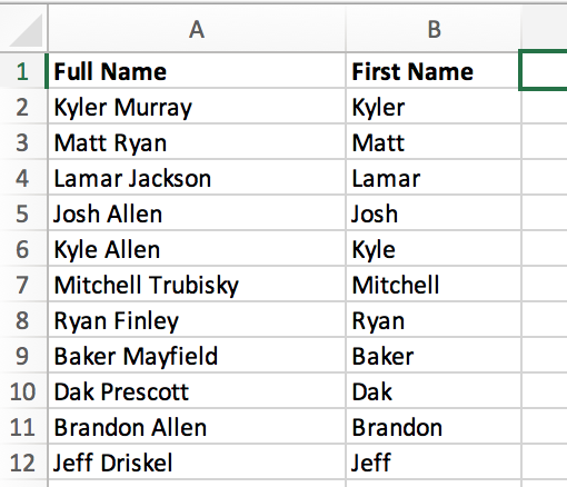
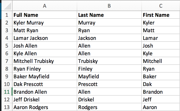
This formula will extract the all the text from cell A1 that occurs before the first space. A great example of this is when you need to extract the first names from a column of full names.
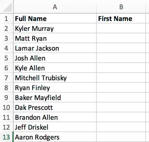
We start with a list of Full Names in Column A, and we want to extract all the First Names to be in Column B.
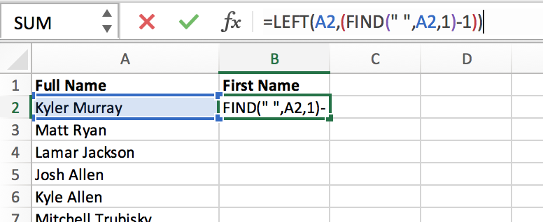
- Select cell B2
- In the function bar, type the formula =LEFT(A2,(FIND(” “,A2,1)-1))
- Press the [Enter] or [Return] key
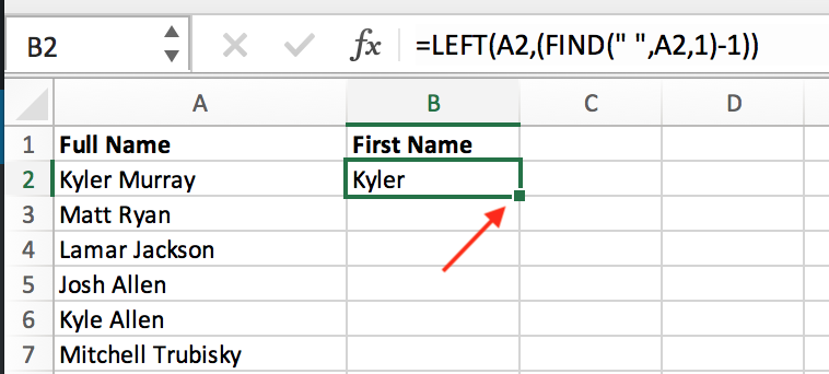
To apply the formula to the entire column, place your cursor in the lower right corner of the cell until you see the little + symbol.
Then just double click, and watch the magic!
Code language: JavaScript (javascript)
=MID(A2,FIND(" ",A2)+1,LEN(A2))
Note: if you need a comma or some other character instead of a space, replace the ” “ part with the character you need wrapped in double quotes.
Extract text after first comma
=MID(A2,FIND(“,”,A2)+1,LEN(A2))
Extract text after first ???
=MID(A2,FIND(“???”,A2)+1,LEN(A2))
This formula will extract the ALL the text from cell A1 that occurs after the first space. A great example of this is when you need to extract the last names from a column of full names.
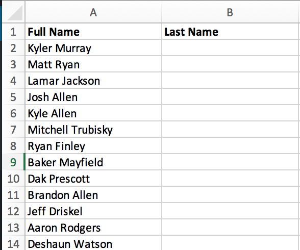
We start with a list of Full Names in Column A, and we want to extract all the Last Names to be in Column B.
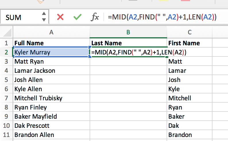
- Select cell B2
- In the function bar, type the formula =MID(A2,FIND(” “,A2)+1,LEN(A2))
- Press the [Enter] or [Return] key
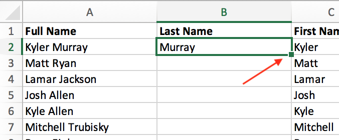
To apply the formula to the entire column, place your cursor in the lower right corner of the cell until you see the little + symbol.
Then just double click, and watch the magic!
Code language: JavaScript (javascript)
=LEFT(A2, SEARCH(" ", A2, SEARCH(" ", A2) + 1))
That complex formula above will get ALL the text from cell A2 that occurs before the second space.
If you need to get a specific word from a string with commas instead, then just replace ” “ with “,”. Like this formula below:
Code language: JavaScript (javascript)
=LEFT(A2, SEARCH(",", A2, SEARCH(",", A2) + 1))
Note: the code above will include the trailing comma. If you need to strip off the last comma, then use this instead:
Code language: JavaScript (javascript)
=LEFT(A2, SEARCH(",", A2, SEARCH(",", A2) + 1)-1)
Pro Tip: Once you have the formula entered in properly, you can very quickly apply it to the entire column: (scroll up to the previous sections for “How To” screenshots)
- Move cursor to bottom right hand corner of cell (with formula already entered)
- When you see the little + symbol, double click
Code language: JavaScript (javascript)
=RIGHT(A2, LEN(A2) - (SEARCH(" ", A2, SEARCH(" ", A2) + 1)))
The code above will extract ALL text after the second space from cell A2.
If you need to get a specific word from a string with commas instead, then just replace ” ” with “,”. Like this formula below:
Code language: JavaScript (javascript)
=RIGHT(A2, LEN(A2) - (SEARCH(",", A2, SEARCH(",", A2) + 1)))
Pro Tip: Once you have the formula entered in properly, you can very quickly apply it to the entire column: (scroll up to the previous sections for “How To” screenshots)
- Move cursor to bottom right hand corner of cell (with formula already entered)
- When you see the little + symbol, double click
Code language: JavaScript (javascript)
=MID(A2,FIND(" ",A2)+1,FIND(" ",A2,FIND(" ",A2)+1)-FIND(" ",A2))
The code above will extract the string in A2 that is between two spaces. This is ideal when you have a Full Name column (firstName MiddleName lastName) and need to extract only the middle name.
If you need to extract a string from a comma delimited cell, then you could use this formula instead:
Code language: JavaScript (javascript)
=MID(A2,FIND(",",A2)+1,FIND(",",A2,FIND(",",A2)+1)-FIND(",",A2)-1)
Pro Tip: Once you have the formula entered in properly, you can very quickly apply it to the entire column: (scroll up to the previous sections for “How To” screenshots)
- Move cursor to bottom right hand corner of cell (with formula already entered)
- When you see the little + symbol, double click
Anything I missed?
Leave a comment below if there’s anything you wanted to see but didn’t. If you found this article useful, bookmark it for future reference. (And don’t forget to share it with your friends, social media, etc.)
If you want more useful Excel tips coming to your inbox (I promise not to spam you!) then you should signup for the free newsletter!
[sibwp_form id=2]
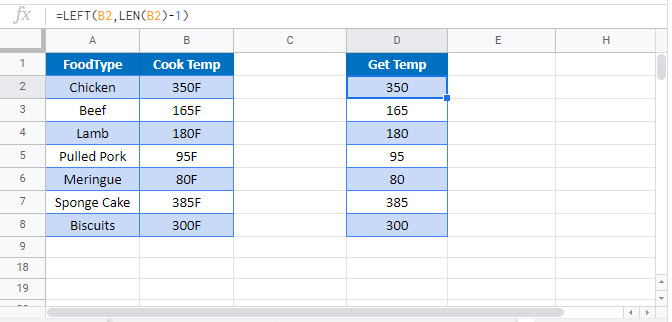
This tutorial will demonstrate how to extract text from a cell in Excel and Google Sheets.
Extract Text from Left
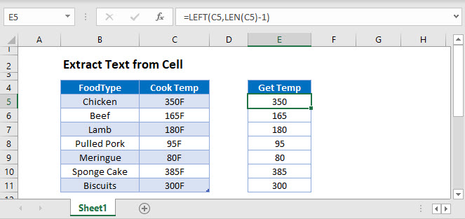
You can extract text from the left side of a cell in Excel by using the LEFT Function. Simply supply the text, and enter the number of characters to return.
However, this will only extract a fixed number of characters. You can see above some cook temperatures are correct extracted (ex. 300), but some are not (ex. 95F). To create a dynamic formula that will work in all scenarios are we can use the LEN Function, combined with the LEFT Function.
LEN Function – Count Characters in a Cell
Use the LEN Function to count the number of characters in the cell:
=LEN(C3)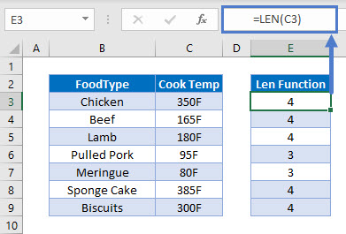
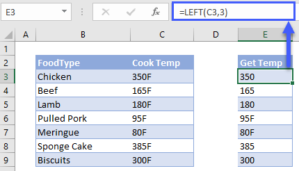
LEFT Function – Show Characters from the Left
Then, create a new LEFT Function that extracts a number of characters determined by the LEN Function created above.
=LEFT(C3, E3-1)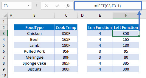
Combining these functions looks like this:
=LEFT(C3,LEN(C3)-1)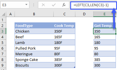
RIGHT and LEN Functions
Similarly, we can also extract characters from the right of a cell by using the RIGHT Function to return a certain number of characters from the right.
=RIGHT(C3,LEN(C3)-n)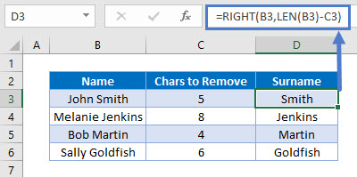
MID and SEARCH Functions
In the next section, we will use the SEARCH and MID functions to extract characters from the middle of a text string.
=MID(B3,SEARCH(" ",B3)+1,999)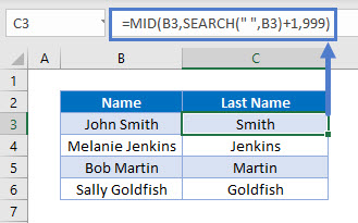
SEARCH Function
First, we use the SEARCH Function to find the position of the space (” “) between the first and last names.
=SEARCH(" ", B3)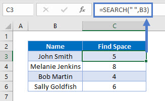
MID Function
Next, we use the MID Function to return all the characters after the space.
- We need to add 1 to the result of the previous formula so that we return the first character after the space.
- We use the large number 999 to return all characters.
=MID(B3, C3+1, 999)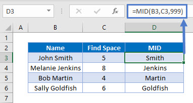
Combining these 2 functions gives us the original formula for the last name.
=MID(B3, SEARCH(B3, " ")+1, 999)
Extract Text Before or After a Specific Character
You can also use the LEFT, RIGHT, LEN and SEARCH functions to extract the text before or after a specific character. In this case we will separate first and last names.
Extract Text Before Character
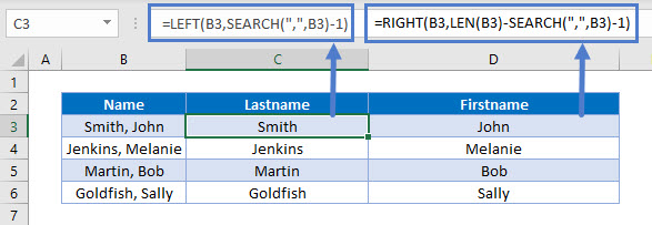
First, we can use the SEARCH Function to find the position of the comma in the text string.
=SEARCH(",", B3)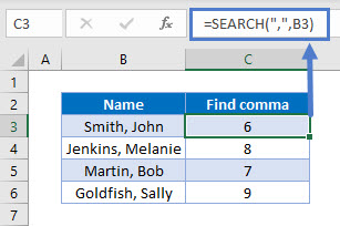
Next, we can use the LEFT function to extract the text before the position of the comma.
- We need to subtract 1 from the position of the comma so not to include the comma in our result.
=LEFT(B3, SEARCH(",",B3)-1)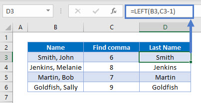
Combining these 2 functions gives us the original formula for the last name.
Extract Text After Character
=RIGHT(B3,LEN(B3)-SEARCH(",",B3)-1)
In addition to using the SEARCH function once again, we also use the LEN function in conjunction with the RIGHT function to get extract text after a specific character.
The LEN Function is to get the length of the text in B3, while the SEARCH function is once again used to find the position of the comma. We then use the RIGHT function to extract the characters after the comma in the text string.
Extract Text From Middle of Text String
Next, we will discuss how to extract text from the middle of a text string
To extract text from the middle of a text string, we can use the RIGHT, SEARCH and LEN functions to get the text from the right side of the string, and then use the MID and LEN functions to get the text in the middle. We will also incorporate the TRIM function to trim any spaces on either side of the text string.
=RIGHT(B3,LEN(B3)-SEARCH(" ",B3)-LEN(TRIM(MID(B3,SEARCH(" ",B3,1)+1,
SEARCH(" ",B3,SEARCH(" ",B3,1)+1)-SEARCH(" ",B3,1))))-1)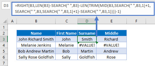
This formula will only work if there is more than one space in the text string. If there is only one space, an error with #VALUE would be returned.
To solve this problem, for names without middle names or initials, we can use the original formula using the MID and SEARCH Functions.
=MID(B3,SEARCH(" ",B3)+1,999))We can create a single formula that uses both techniques to handle all situations with the IFERROR Function. (The IFERROR Function performs a calculation. If that calculation results in an error, then another calculation is performed.)
=IFERROR(RIGHT(B3,LEN(B3)-SEARCH(" ",B3)-LEN(TRIM(MID(B3,SEARCH(" ",B3,1)+1,
SEARCH(" ",B3,SEARCH(" ",B3,1)+1)-SEARCH(" ",B3,1))))-1),MID(B3,SEARCH(" ",B3)+1,999))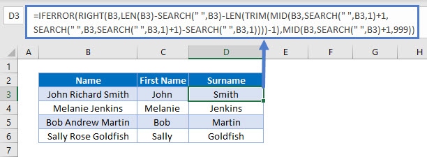
We can then use the MID and LEN functions to obtain the middle name or initial.
=MID(B3,LEN(C3)+1,LEN(B3)-LEN(C3&D3))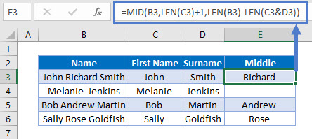
Extract Text From Cell in Google Sheets
All the examples above works the same way in Google Sheets.
Excel has a set of TEXT Functions that can do wonders. You can do all kinds of text slice and dice operations using these functions.
One of the common tasks for people working with text data is to extract a substring in Excel (i.e., get psrt of the text from a cell).
Unfortunately, there is no substring function in Excel that can do this easily. However, this could still be done using text formulas as well as some other in-built Excel features.
Let’s first have a look at some of the text functions we will be using in this tutorial.
Excel TEXT Functions
Excel has a range of text functions that would make it really easy to extract a substring from the original text in Excel. Here are the Excel Text functions that we will use in this tutorial:
- RIGHT function: Extracts the specified numbers of characters from the right of the text string.
- LEFT function: Extracts the specified numbers of characters from the left of the text string.
- MID function: Extracts the specified numbers of characters from the specified starting position in a text string.
- FIND function: Finds the starting position of the specified text in the text string.
- LEN function: Returns the number of characters in the text string.
Extract a Substring in Excel Using Functions
Suppose you have a dataset as shown below:
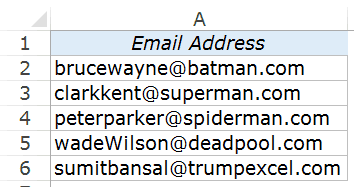
These are some random (but superhero-ish) email ids (except mine), and in the examples below, I’ll show you how to extract the username and domain name using the Text functions in Excel.
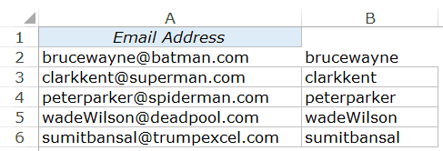
Example 1 – Extracting Usernames from Email Ids
While using Text functions, it is important to identify a pattern (if any). That makes it really easy to construct a formula. In the above case, the pattern is the @ sign between the username and the domain name, and we will use it as a reference to get the usernames.
Here is the formula to get the username:
=LEFT(A2,FIND("@",A2)-1)
The above formula uses the LEFT function to extract the username by identifying the position of the @ sign in the id. This is done using the FIND function, which returns the position of the @.
For example, in the case of brucewayne@batman.com, FIND(“@”,A2) would return 11, which is its position in the text string.
Now we use the LEFT function to extract 10 characters from the left of the string (one less than the value returned by the LEFT function).
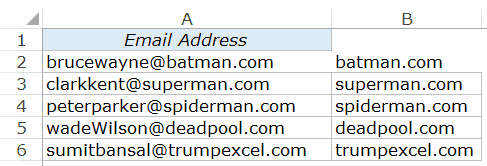
Example 2 – Extracting the Domain Name from Email Ids
The same logic used in the above example can be used to get the domain name. A minor difference here is that we need to extract the characters from the right of the text string.
Here is the formula that will do this:
=RIGHT(A2,LEN(A2)-FIND("@",A2))
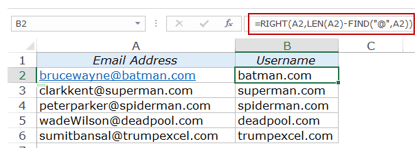
In the above formula, we use the same logic, but adjust it to make sure we are getting the correct string.
Let’s again take the example of brucewayne@batman.com. The FIND function returns the position of the @ sign, which is 11 in this case. Now, we need to extract all the characters after the @. So we identify the total length of the string and subtract the number of characters till the @. It gives us the number of characters that cover the domain name on the right.
Now we can simply use the RIGHT function to get the domain name.
Example 3 – Extracting the Domain Name from Email Ids (without .com)
To extract a substring from the middle of a text string, you need to identify the position of the marker right before and after the substring.
For example, in the example below, to get the domain name without the .com part, the marker would be @ (which is right before the domain name) and . (which is right after it).
Here is the formula that will extract the domain name only:
=MID(A2,FIND("@",A2)+1,FIND(".",A2)-FIND("@",A2)-1)
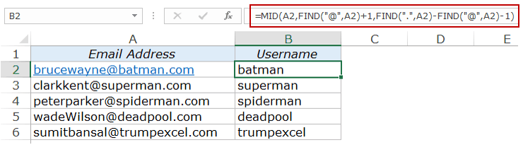
Excel MID function extracts the specified number of characters from the specified starting position. In this example above, FIND(“@”,A2)+1 specifies the starting position (which is right after the @), and FIND(“.”,A2)-FIND(“@”,A2)-1 identifies the number of characters between the ‘@‘ and the ‘.‘
Update: One of the readers William19 mentioned that the above formula wouldn’t work in case there is a dot(.) in the email id (for example, bruce.wayne@batman.com). So here is the formula to deal with such cases:
=MID(A1,FIND("@",A1)+1,FIND(".",A1,FIND("@",A1))-FIND("@",A1)-1)
Using Text to Columns to Extract a Substring in Excel
Using functions to extract a substring in Excel has the advantage of being dynamic. If you change the original text, the formula would automatically update the results.
If this is something you may not need, then using the Text to Columns feature could be a quick and easy way to split the text into substrings based on specified markers.
Here is how to do this:
This will instantly give you two sets of substrings for each email id used in this example.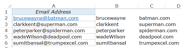
If you want to further split the text (for example, split batman.com to batman and com), repeat the same process with it.
Using FIND and REPLACE to Extract Text from a Cell in Excel
FIND and REPLACE can be a powerful technique when you are working with text in Excel. In the examples below, you’ll learn how to use FIND and REPLACE with wildcard characters to do amazing things in Excel.
See Also: Learn All about Wildcard Characters in Excel.
Let’s take the same Email ids examples.
Example 1 – Extracting Usernames from Email Ids
Here are the steps to extract usernames from Email Ids using the Find and Replace functionality:
This will instantly remove all the text before the @ in the email ids. You’ll have the result as shown below:
How this works?? – In the above example, we have used a combination of @ and *. An asterisk (*) is a wildcard character that represents any number of characters. Hence, @* would mean, a text string that starts with @ and can have any number of characters after it. For example in brucewayne@batman.com, @* would be @batman.com. When we replace @* with blank, it removes all the characters after @ (including @).
Example 2 – Extracting the Domain Name from Email Ids
Using the same logic, you can modify the ‘Find what’ criteria to get the domain name.
Here are the steps:
This will instantly remove all the text before the @ in the email ids. You’ll have the result as shown below:
You May Also Like the Following Excel Tutorials:
- How to Count Cells that Contain Text Strings.
- Extract Usernames from Email Ids in Excel [2 Methods].
- Excel Functions (Examples + Videos).
- Get More Out of Find and Replace in Excel.
- How to Capitalize First Letter of a Text String in Excel
- How to Extract the First Word from a Text String in Excel
- Separate Text and Numbers in Excel