
Use the GETPIVOTDATA function to query an existing Pivot Table and retrieve specific data based on the pivot table structure. The advantage of GETPIVOTDATA over a simple cell reference is that it collects data based on structure, not cell location. GETPIVOTDATA will continue to work correctly even when a pivot table changes, as long as the field(s) being referenced is still present.
The first argument, data_field, names a value field to query. The second argument, pivot_table, is a reference to any cell in an existing pivot table. Additional arguments are supplied in field/item pairs that act like filters to limit the data retrieved based on the structure of the pivot table. For example, you might supply the field «Region» with the item «East» to limit sales data to Sales in the East Region.
The GETPIVOTDATA function is generated automatically when you reference a value cell in a pivot table by pointing and clicking. To avoid this, you can simply type the address of the cell you want (instead of clicking). If you want to disable this feature entirely, disable «Generate GETPIVOTDATA» in the menu at Pivot TableTools > Options > Options (far left, below the pivot table name).
Examples
The examples below are based on the following pivot table:

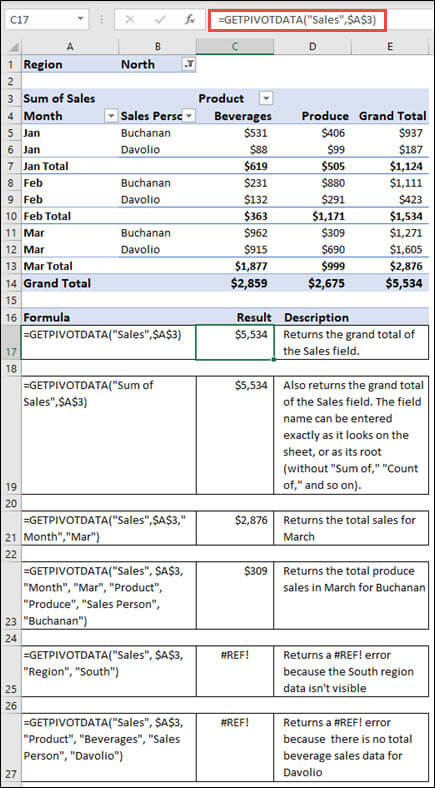
The first argument in the GETPIVOTDATA function names the field from which to retrieve data. The second argument is a reference to a cell that is part of the pivot table. To get total Sales from the pivot table shown:
=GETPIVOTDATA("Sales",$B$4) // returns 138602
Fields and item pairs are supplied in pairs entered as text values. To get total sales for the Product Hazelnut:
=GETPIVOTDATA("Sales",$B$4,"Product","Hazelnut") // returns 62456
To get total Sales for the West region:
=GETPIVOTDATA("Sales",$B$4,"Region","West") // returns 41518
To get total sales for Almond in the East region, you can use either of the formulas below:
=GETPIVOTDATA("Sales",$B$4,"Region","East","Product","Almond")
=GETPIVOTDATA("Sales",$B$4,"Product","Almond","Region","East")
You can also use cell references to provide field and item names. In the example shown above, the formula in I8 is:
=GETPIVOTDATA("Sales",$B$4,"Region",I6,"Product",I7)
The values for Region and Product come from cells I5 and I6. The data is collected based on the region «Midwest» in cell I6 for the product «Hazelnut» in cell I7.
Dates and times
When using GETPIVOTDATA to fetch information from a pivot table based on a date or time date or time, use Excel’s native format, or a function like the DATE function. For example, to get total Sales on April 1, 2021 when individual dates are displayed:
=GETPIVOTDATA("Sales",A1,"Date",DATE(2021,4,1))
When dates are grouped, refer to the group names as text. For example, if the Date field is grouped by year:
=GETPIVOTDATA("Sales",A1,"Year","2021")
Notes
- The name of the data_field, and field/item values must be enclosed in double quotes («)
- GETPIVOTDATA will return a #REF error if any fields are spelled incorrectly.
- GETPIVOTDATA will return a #REF error if the reference to pivot_table is not valid.
Excel for Microsoft 365 Excel for Microsoft 365 for Mac Excel for the web Excel 2021 Excel 2021 for Mac Excel 2019 Excel 2019 for Mac Excel 2016 Excel 2016 for Mac Excel 2013 Excel 2010 Excel 2007 Excel for Mac 2011 Excel Starter 2010 More…Less
The GETPIVOTDATA function returns visible data from a PivotTable.
In this example, =GETPIVOTDATA(«Sales»,A3) returns the total sales amount from a PivotTable:

Syntax
GETPIVOTDATA(data_field, pivot_table, [field1, item1, field2, item2], …)
The GETPIVOTDATA function syntax has the following arguments:
|
Argument |
Description |
|---|---|
|
data_field Required |
The name of the PivotTable field that contains the data that you want to retrieve. This needs to be in quotes. |
|
pivot_table Required |
A reference to any cell, range of cells, or named range of cells in a PivotTable. This information is used to determine which PivotTable contains the data that you want to retrieve. |
|
field1, item1, field2, item2… Optional |
1 to 126 pairs of field names and item names that describe the data that you want to retrieve. The pairs can be in any order. Field names and names for items other than dates and numbers need to be enclosed in quotation marks. For OLAP PivotTables, items can contain the source name of the dimension and also the source name of the item. A field and item pair for an OLAP PivotTable might look like this: «[Product]»,»[Product].[All Products].[Foods].[Baked Goods]» |
Notes:
-
You can quickly enter a simple GETPIVOTDATA formula by typing = (the equal sign) in the cell you want to return the value to and then clicking the cell in the PivotTable that contains the data you want to return.
-
You can turn this feature off by selecting any cell within an existing PivotTable, then go to the PivotTable Analyze tab > PivotTable > Options > Uncheck the Generate GetPivotData option.
-
Calculated fields or items and custom calculations can be included in GETPIVOTDATA calculations.
-
If the pivot_table argument is a range that includes two or more PivotTables, data will be retrieved from whichever PivotTable was created most recently.
-
If the field and item arguments describe a single cell, then the value of that cell is returned regardless of whether it is a string, number, error, or blank cell.
-
If an item contains a date, the value must be expressed as a serial number or populated by using the DATE function so that the value will be retained if the worksheet is opened in a different locale. For example, an item referring to the date March 5, 1999 could be entered as 36224 or DATE(1999,3,5). Times can be entered as decimal values or by using the TIME function.
-
If the pivot_table argument is not a range in which a PivotTable is found, GETPIVOTDATA returns #REF!.
-
If the arguments do not describe a visible field, or if they include a report filter in which the filtered data is not displayed, GETPIVOTDATA returns the #REF! error value.
Examples
The formulas in the example below show various methods for getting data from a PivotTable.
Top of Page
Need more help?
You can always ask an expert in the Excel Tech Community or get support in the Answers community.
See Also
Excel functions (alphabetical)
Excel functions (by category)
Need more help?

Описание
Синтаксис и аргументы
Использование и примеры
- Пример 1: базовое использование GETPIVOTDATA функция
- Пример 2: Как избежать значений ошибок, если аргументом является дата или время в GETPIVOTDATA функция
Описание
Наблюдения и советы этой статьи мы подготовили на основании опыта команды GETPIVOTDATA функция запрашивает сводную таблицу и возвращает данные на основе структуры сводной таблицы.
Синтаксис и аргументы
Синтаксис формулы
=GETPIVOTDATA (data_field, pivot_table, [field1, item1], …)
аргументы
- Data_field: Необходимые. Имя поля заключено в двойные квоты и содержит данные, которые вы хотите вернуть.
- Pivot_table: Необходимые. Ячейка или диапазон ячеек или именованный диапазон, используемый для определения, из какой сводной таблицы вы будете извлекать данные.
- Field1, item1: Необязательный. От 1 до 126 пар имен полей и имен элементов, которые указывают на данные, которые вы хотите получить. Если имена полей и имена элементов не являются числовыми значениями, вам необходимо заключить их в кавычки.
Возвращаемое значение
Функция GETPIVOTDATA возвращает данные, хранящиеся в данной сводной таблице.
Замечания
1) Вычисляемые поля и пользовательские вычисления, такие как общая сумма и сумма каждого результата, также могут быть аргументами в GETPIVOTDATA функции.
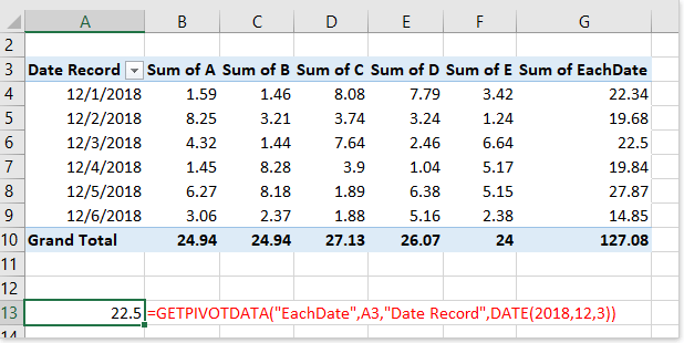
2) Если элемент содержит дату или время, возвращаемое значение может быть потеряно, если книгу переместить в другое место и отобразить как значение ошибки #REF !. Чтобы избежать этого случая, вы можете выразить дату или время как порядковый номер, например show 12/3/2018 как 43437.
3) Если аргумент pivot_table не является ячейкой или диапазоном, в котором находится сводная таблица, GETPIVOTDATA возвращает #REF !.
4) Если аргументы не видны в данной сводной таблице, GETPIVOTDATA функция возвращает # ССЫЛКУ! значение ошибки.
Использование и примеры
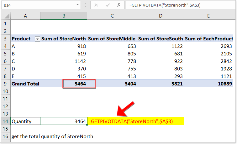
Пример 1: базовое использование GETPIVOTDATA функция
1) Только первые два обязательных аргумента:
=GETPIVOTDATA(«StoreNorth»,$A$3)
Объясните:
Если есть только два аргумента в GETPIVOTDARA функция, она автоматически возвращает значения в поле Grand Total в зависимости от имени данного элемента. В моем примере он возвращает общее количество полей StoreNorth в сводной таблице, которое помещается в диапазон A3: E9 (начинается с ячейки A3).
2) С аргументом data_field, pivot_table, field1, item1
=GETPIVOTDATA(«StoreNorth»,$A$3,»Product»,»B»)
Объясните:
Юг, север: data_field, поле, из которого вы хотите получить значение;
A3: pivot_table, первая ячейка сводной таблицы — это ячейка A3;
Продукт, B: filed_name, item_name, пара, которая описывает, какое значение вы хотите вернуть.

Пример 2: Как избежать значений ошибок, если аргументом является дата или время в GETPIVOTDATA функция
Если аргументы в GETPIVOTDATA содержат дату или время, результат может быть изменен на значение ошибки # ССЫЛКА! пока книга открыта в другом месте, как показано ниже:
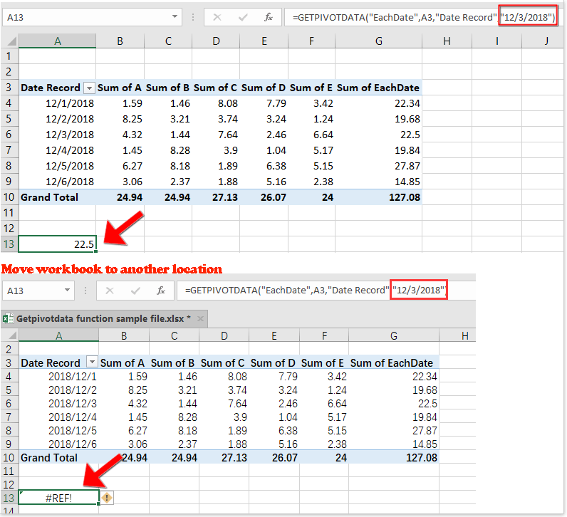
В этом случае вы можете
1) Используйте DATEVALUE функция
=GETPIVOTDATA(«EachDate»,A3,»Date Record»,DATEVALUE(«12/3/2018»))
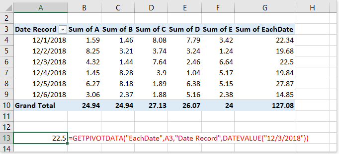
2) Используйте DATE функция
=GETPIVOTDATA(«EachDate»,A3,»Date Record»,DATE(2018,12,3))
3) Обратитесь к ячейке с датой
=GETPIVOTDATA(«EachDate»,A3,»Date Record»,A12)

Файл примера

Лучшие инструменты для работы в офисе
Kutools for Excel — Помогает вам выделиться из толпы
Хотите быстро и качественно выполнять свою повседневную работу? Kutools for Excel предлагает 300 мощных расширенных функций (объединение книг, суммирование по цвету, разделение содержимого ячеек, преобразование даты и т. д.) и экономит для вас 80 % времени.
- Разработан для 1500 рабочих сценариев, помогает решить 80% проблем с Excel.
- Уменьшите количество нажатий на клавиатуру и мышь каждый день, избавьтесь от усталости глаз и рук.
- Станьте экспертом по Excel за 3 минуты. Больше не нужно запоминать какие-либо болезненные формулы и коды VBA.
- 30-дневная неограниченная бесплатная пробная версия. 60-дневная гарантия возврата денег. Бесплатное обновление и поддержка 2 года.
")
Вкладка Office — включение чтения и редактирования с вкладками в Microsoft Office (включая Excel)
- Одна секунда для переключения между десятками открытых документов!
- Уменьшите количество щелчков мышью на сотни каждый день, попрощайтесь с рукой мыши.
- Повышает вашу продуктивность на 50% при просмотре и редактировании нескольких документов.
- Добавляет эффективные вкладки в Office (включая Excel), точно так же, как Chrome, Firefox и новый Internet Explorer.
")
Pivot tables are very powerful analysis tools. They can summarize vast amounts of data with just few clicks. But they are lousy when it comes to output. Imagine the horror of putting a pivot table right inside your beautiful dashboard. One refresh could ruin the layout and create half-an-hour extra work for you.
How to combine the power of pivot tables with elegance of your dashboards?
The answer is: GETPIVOTDATA()
What is GETPIVOTDATA?
As the name suggests, GETPIVOTDATA gets pivot table data. The best way to understand GETPIVOTDATA is by looking at an example.
Let’s say, you have a pivot table like the one below. And you want to know what is the Amount for Cust Area = Middle & Prod Category = Biscuits combination.
The below GETPIVOTDATA formula should work.
=GETPIVOTDATA(“Amount”,$A$3,”Cust Area”,”Middle“,”Prod Category”,”Biscuits“)

As you can see GETPIVOTDATA has below syntax.
GETPIVOTDATA(value field name, any cell reference in pivot table, [field name 1, value1, field name 2, value 2 …])
Few more examples of GETPIVOTDATA:
Check out below examples to understand how various parameters of the GETPIVOTDATA function behave:
| GETPIVOTDATA function | What it does | Value |
|---|---|---|
| =GETPIVOTDATA(“Amount”,$A$3,”Cust Area”,”South”,”Prod Category”,”Biscuits”) | Gets Amount for South & Biscuits combination | $609.50 |
| =GETPIVOTDATA(“Amount”,$A$3,”Prod Category”,”Biscuits”) | Gets grand total for Biscuits | $5,251.10 |
| =GETPIVOTDATA(“Amount”,$A$3,”Cust Area”,”South”) | Gets grand total for South | $4,342.20 |
| =GETPIVOTDATA(“Amount”,$A$3) | Gets grand total of all amounts | $41,828.00 |
| =GETPIVOTDATA(“Amount”,$A$1,”Cust Area”,”West”,”Prod Category”,”Snacks”) | Gives an error as $A$1 is not part of the pivot | #REF! |
| =GETPIVOTDATA(“Amount”,$A$3,”Cust Area”,$P$2,”Prod Category”,$P$3) | Gets Amount for cust area = P2 and pro category = P3 cell values. | depends on variables |
| =GETPIVOTDATA(“Amount”,$A$3,”Prod Category”,category_name) | Gets grand total for category = category_name value | depends on variables |
| =GETPIVOTDATA($P$4&””,$A$3,”Cust Area”,$P$2,”Prod Category”,$P$3) | Gets P4 value field for Cust Area = P2 and Prod Category = P3. Note: $P$4 &”” is used to convince GPD that P4 is a string not number. |
depends on variables |
Using GETPIVOTDATA in dashboards
The idea is simple. Since GETPIVOTDATA can be parameterized with variable cells or named ranges, we can use it in dashboards to get relevant data based on user input.
Sample this:

Or this dashboard powered with GETPIVOTDATA

Things to note when working with GETPIVOTDATA:
GETPIVOTDATA is a very useful function, but it does have a few quirks.
- If your pivot table has slicers linked to them, GPD will reflect the results based on slicer selection.
- If your pivot table has any items filtered (say category Biscuits is filtered out), then GPD will return #REF error when you try to get any value corresponding to Biscuits.
- If you change the pivot table structure, your GETPIVOTDATA functions may not work as you expect.
- If you turn off grand totals or sub-totals, you can no longer get them thru GPD.
- GPD requires that your original pivot tables remain intact and visible all the time.
- If you want to completely get rid of pivot tables and still get answers to questions, then you should use CUBE formulas along with Workbook data model feature (more on this in a future post).
- The best & easiest way to write GPD is by pressing = and referencing a cell inside the pivot. This will automatically write the GPD for you. You can then customize the parameters as you need.
- You can turn-off GPD by going to Pivot Table Analyze ribbon tab & unchecking “Generating GETPIVODATA” option from PivotTable options area.
Download GETPIVOTDATA Examples workbook
Please click here to download the GETPIVOTDATA example workbook. Refer to various tabs & formulas to learn more. Don’t forget to play with the dashboard powered by GETPIVOTDATA.
Learn more about Pivot Tables
If you are new to Pivot Tables, it’s high time you started using them. Check out below pages and get started.
- Introduction to Excel Pivot Tables – article , Podcast
- Comprehensive guide to Excel Pivot Tables
- Slicers – Introduction, what are they, advanced scenarios
- Building dashboards with Pivot Tables + Slicers
- Convert regular pivots to GETPIVOTDATA – 3 part tutorial from Mike Alexander, part 2 & part 3
How do you use GETPIVOTDATA?
Let me be honest. For my dashboards, I usually write direct cell references (=A7) instead of GPD. This keeps my formulas short. For dynamic / parameterized setups, I usually write INDEX / MATCH formulas that talk to Pivot Table data. But occasionally I use GETPIVOTDATA because it is very easy to setup and does what it says on the sticker.
What about you? How do you use GETPIVOTDATA? Please share scenarios in the comments section.
Share this tip with your colleagues

Get FREE Excel + Power BI Tips
Simple, fun and useful emails, once per week.
Learn & be awesome.
-
12 Comments -
Ask a question or say something… -
Tagged under
advanced excel, awesome august, dashboards, data validation, downloads, GETPIVOTDATA, Microsoft Excel Formulas, pivot tables, screencasts, slicers
-
Category:
Pivot Tables & Charts

Welcome to Chandoo.org
Thank you so much for visiting. My aim is to make you awesome in Excel & Power BI. I do this by sharing videos, tips, examples and downloads on this website. There are more than 1,000 pages with all things Excel, Power BI, Dashboards & VBA here. Go ahead and spend few minutes to be AWESOME.
Read my story • FREE Excel tips book


Excel School made me great at work.
5/5

From simple to complex, there is a formula for every occasion. Check out the list now.

Calendars, invoices, trackers and much more. All free, fun and fantastic.

Power Query, Data model, DAX, Filters, Slicers, Conditional formats and beautiful charts. It’s all here.

Still on fence about Power BI? In this getting started guide, learn what is Power BI, how to get it and how to create your first report from scratch.
Related Tips
12 Responses to “How to use GETPIVOTDATA with Excel Pivot Tables”
-
 Jeff S says:
 I started using CUBEVALUE
-
Jeff S says:
We started using CUBEVALUE (and related) formulas recently with much success. From what I’ve seen and read, they’re much easier to work with than GPD. Philip J. Taylor of http://www.excelcraft.com has some excellent material.
-
Jason says:
Does anyone know how to use getpivotdata or something similar for powerpivot created pivot tables?
-
Good lord! I’m working on a project right now that could use this. Thanks for this blogpost!!
-
Jeff Weir says:
Chandoo: re If you change the pivot table structure, your GETPIVOTDATA functions may not work as you expect.
The actual beauty of GETPIVOTDATA is that you can change the structure, and still get what you expect. The only time that I’m aware of that you’d get something different is if you dragged field in or out of the PivotTable. But move the existing fields around, and you should get the exact same result no matter where they are.
-
Jeff Weir says:
A problem with GETPIVOTDATA is that it can only be used to reference cells in the DATA area of the PivotTable, and that you can only reference one cell at a time and not an entire field.
But that’s where my home-made Structured PivotTable References functionality comes in handy:
http://chandoo.org/wp/2014/10/18/introducing-structured-references-for-pivottables/
I’m in the process of revising this code to make it super robust, and will update that article with the revised code in the next week or so.
-
Nikki says:
Thank you for making August so awesome, Chandoo!
I am learning a lot and being reminded of what I have already forgotten 🙂
You are awesome!
-
Tom says:
This is really helpful and easy to understand.
-
Shashidhar says:
Hi Guys,
Is it possible to return a text instead of only numbers.
-
vijay says:
=GETPIVOTDATA(«Amount»,$A$3,»Cust Area»,»South»,»Prod Category»,»Biscuits»)
not working
Leave a Reply
Возвращает данные, хранящиеся в отчете сводной таблицы. Функцию ПОЛУЧИТЬ.ДАННЫЕ.СВОДНОЙ.ТАБЛИЦЫ можно использовать для извлечения итоговых данных из отчета сводной таблицы, если они отображаются в отчете.
Описание функции
Возвращает данные, хранящиеся в отчете сводной таблицы. Функцию ПОЛУЧИТЬ.ДАННЫЕ.СВОДНОЙ.ТАБЛИЦЫ можно использовать для извлечения итоговых данных из отчета сводной таблицы, если они отображаются в отчете.
Можно быстро ввести простую формулу ПОЛУЧИТЬ.ДАННЫЕ.СВОДНОЙ.ТАБЛИЦЫ, введя = (знак равенства) в ячейку, в которую должно быть возвращено значение, и затем щелкнув ячейку в отчете сводной таблицы, содержащем необходимые данные.
Синтаксис
=ПОЛУЧИТЬ.ДАННЫЕ.СВОДНОЙ.ТАБЛИЦЫ(поле_данных, сводная_таблица, [поле1, элем1, поле2, элем2], ...)Аргументы
поле_данныхсводная_таблицаполе1, элем1, поле2, элем2
Обязательный аргумент. Заключенное в кавычки имя поля данных, содержащего данные, которые необходимо извлечь.
Обязательный аргумент. Ссылка на ячейку, диапазон ячеек или именованный диапазон ячеек в отчете сводной таблицы. Эти сведения используются для определения отчета сводной таблицы, содержащего данные, которые необходимо извлечь.
Необязательный аргумент. От 1 до 126 пар имен полей и элементов, описывающих данные, которые необходимо извлечь. Они могут следовать друг за другом в произвольном порядке. Имена полей и элементов (кроме дат и чисел) заключаются в кавычки. В отчетах сводных таблиц OLAP элементы могут содержать исходное имя измерения и также исходное имя элемента. Пара «поле-элемент» для сводной таблицы OLAP может выглядеть следующим образом:
[Продукт]";"[Продукт].[Все продукты].[Продовольствие].[Выпечка]"Замечания
- Вычисляемые поля или элементы и дополнительные вычисления включаются в расчеты для функции ПОЛУЧИТЬ.ДАННЫЕ.СВОДНОЙ.ТАБЛИЦЫ.
- Если с помощью аргумента «сводная_таблица» задан диапазон, включающий несколько отчетов сводных таблиц, данные будут извлекаться из того отчета, который был создан в диапазоне последним.
- Если аргументы «поле» и «элемент» описывают одну ячейку, возвращается значение, содержащееся в этой ячейке, независимо от его типа (строка, число, ошибка и др.).
- Если аргумент «элемент» содержит дату, необходимо представить это значение как порядковый номер или воспользоваться функцией ДАТА, чтобы это значение не изменилось при открытии листа в системе с другими языковыми настройками. Например, элемент, ссылающийся на дату 5 марта 1999 г., можно ввести двумя способами: 36 224 или ДАТА(1999;3;5). Время можно задать в виде десятичных значений или с помощью функции ВРЕМЯ.
- Если значение аргумента «сводная_таблица» не является диапазоном, содержащим отчет сводной таблицы, функция ПОЛУЧИТЬ.ДАННЫЕ.СВОДНОЙ.ТАБЛИЦЫ возвращает значение ошибки #ССЫЛКА!.
- Если аргументы не описывают видимое поле или содержат фильтр отчета, в котором не отображаются отфильтрованные данные, функция ПОЛУЧИТЬ.ДАННЫЕ.СВОДНОЙ.ТАБЛИЦЫ возвращает значение ошибки #ССЫЛКА!.
Пример
If you are reading this tutorial, there is a big chance you have heard of (or even used) the Excel Pivot Table. It’s one of the most powerful features in Excel (no kidding).
The best part about using a Pivot Table is that even if you don’t know anything in Excel, you can still do pretty awesome things with it with a very basic understanding of it.
Let’s get started.
Click here to download the sample data and follow along.
What is a Pivot Table and Why Should You Care?
A Pivot Table is a tool in Microsoft Excel that allows you to quickly summarize huge datasets (with a few clicks).
Even if you’re absolutely new to the world of Excel, you can easily use a Pivot Table. It’s as easy as dragging and dropping rows/columns headers to create reports.
Suppose you have a dataset as shown below:
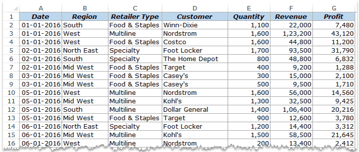
This is sales data that consists of ~1000 rows.
It has the sales data by region, retailer type, and customer.
Now your boss may want to know a few things from this data:
- What were the total sales in the South region in 2016?
- What are the top five retailers by sales?
- How did The Home Depot’s performance compare against other retailers in the South?
You can go ahead and use Excel functions to give you the answers to these questions, but what if suddenly your boss comes up with a list of five more questions.
You’ll have to go back to the data and create new formulas every time there is a change.
This is where Excel Pivot Tables comes in really handy.
Within seconds, a Pivot Table will answer all these questions (as you’ll learn below).
But the real benefit is that it can accommodate your finicky data-driven boss by answering his questions immediately.
It’s so simple, you may as well take a few minutes and show your boss how to do it himself.
Hopefully, now you have an idea of why Pivot Tables are so awesome. Let’s go ahead and create a Pivot Table using the data set (shown above).
Inserting a Pivot Table in Excel
Here are the steps to create a pivot table using the data shown above:
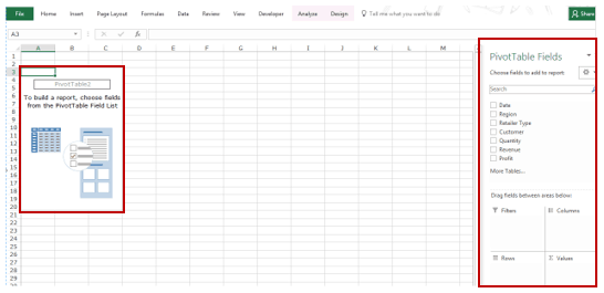
As soon as you click OK, a new worksheet is created with the Pivot Table in it.
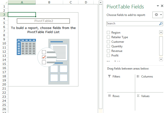
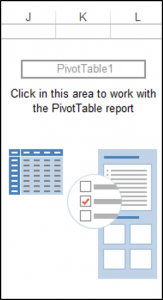
While the Pivot Table has been created, you’d see no data in it. All you’d see is the Pivot Table name and a single line instruction on the left, and Pivot Table Fields on the right.
Now before we jump into analyzing data using this Pivot Table, let’s understand what are the nuts and bolts that make an Excel Pivot Table.
Also read: 10 Excel Pivot Table Keyboard Shortcuts
The Nuts & Bolts of an Excel Pivot Table
To use a Pivot Table efficiently, it’s important to know the components that create a pivot table.
In this section, you’ll learn about:
- Pivot Cache
- Values Area
- Rows Area
- Columns Area
- Filters Area
Pivot Cache
As soon as you create a Pivot Table using the data, something happens in the backend. Excel takes a snapshot of the data and stores it in its memory. This snapshot is called the Pivot Cache.
When you create different views using a Pivot Table, Excel does not go back to the data source, rather it uses the Pivot Cache to quickly analyze the data and give you the summary/results.
The reason a pivot cache gets generated is to optimize the pivot table functioning. Even when you have thousands of rows of data, a pivot table is super fast in summarizing the data. You can drag and drop items in the rows/columns/values/filters boxes and it will instantly update the results.
Note: One downside of pivot cache is that it increases the size of your workbook. Since it’s a replica of the source data, when you create a pivot table, a copy of that data gets stored in the Pivot Cache.
Read More: What is Pivot Cache and How to Best Use It.
Values Area
The Values Area is what holds the calculations/values.
Based on the data set shown at the beginning of the tutorial, if you quickly want to calculate total sales by region in each month, you can get a pivot table as shown below (we’ll see how to create this later in the tutorial).
The area highlighted in orange is the Values Area.
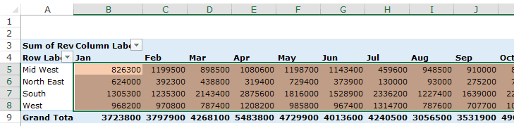
In this example, it has the total sales in each month for the four regions.
Rows Area
The headings to the left of the Values area makes the Rows area.
In the example below, the Rows area contains the regions (highlighted in red):
Columns Area
The headings at the top of the Values area makes the Columns area.
In the example below, Columns area contains the months (highlighted in red):
Filters Area
Filters area is an optional filter that you can use to further drill down in the data set.
For example, if you only want to see the sales for Multiline retailers, you can select that option from the drop down (highlighted in the image below), and the Pivot Table would update with the data for Multiline retailers only.
Analyzing Data Using the Pivot Table
Now, let’s try and answer the questions by using the Pivot Table we have created.
Click here to download the sample data and follow along.
To analyze data using a Pivot Table, you need to decide how you want the data summary to look in the final result. For example, you may want all the regions in the left and the total sales right next to it. Once you have this clarity in mind, you can simply drag and drop the relevant fields in the Pivot Table.
In the Pivot Tabe Fields section, you have the fields and the areas (as highlighted below):
The Fields are created based on the backend data used for the Pivot Table. The Areas section is where you place the fields, and according to where a field goes, your data is updated in the Pivot Table.
It’s a simple drag and drop mechanism, where you can simply drag a field and put it in one of the four areas. As soon as you do this, it will appear in the Pivot Table in the worksheet.
Now let’s try and answer the questions your manager had using this Pivot Table.
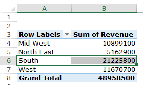
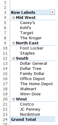
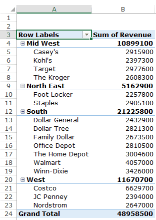
Q1: What were the total sales in the South region?
Drag the Region field in the Rows area and the Revenue field in the Values area. It would automatically update the Pivot Table in the worksheet.
Note that as soon as you drop the Revenue field in the Values area, it becomes Sum of Revenue. By default, Excel sums all the values for a given region and shows the total. If you want, you can change this to Count, Average, or other statistics metrics. In this case, the sum is what we needed.
The answer to this question would be 21225800.
Q2 What are the top five retailers by sales?
Drag the Customer field in the Row area and Revenue field in the values area. In case, there are any other fields in the area section and you want to remove it, simply select it and drag it out of it.
You’ll get a Pivot Table as shown below:
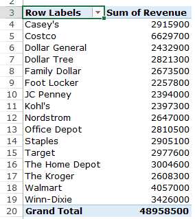
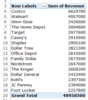
Note that by default, the items (in this case the customers) are sorted in an alphabetical order.
To get the top five retailers, you can simply sort this list and use the top five customer names. To do this:
This will give you a sorted list based on total sales.
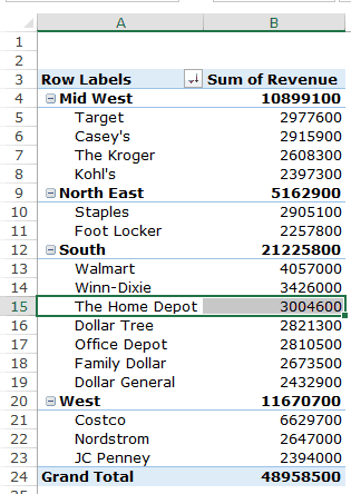
Q3: How did The Home Depot’s performance compare against other retailers in the South?
You can do a lot of analysis for this question, but here let’s just try and compare the sales.
Drag the Region Field in the Rows area. Now drag the Customer field in the Rows area below the Region field. When you do this, Excel would understand that you want to categorize your data first by region and then by customers within the regions. You’ll have something as shown below:
Now drag the Revenue field in the Values area and you’ll have the sales for each customer (as well as the overall region).
You can sort the retailers based on the sales figures by following the below steps:
- Right-click on a cell that has the sales value for any retailer.
- Go to Sort –> Sort Largest to Smallest.
This would instantly sort all the retailers by the sales value.
Now you can quickly scan through the South region and identify that The Home Depot sales were 3004600 and it did better than four retailers in the South region.
Now there are more than one ways to skin the cat. You can also put the Region in the Filter area and then only select the South Region.
Click here to download the sample data.
I hope this tutorial gives you a basic overview of Excel Pivot Tables and helps you in getting started with it.
Here are some more Pivot Table Tutorials you may like:
- Preparing Source Data For Pivot Table.
- How to Apply Conditional Formatting in a Pivot Table in Excel.
- How to Group Dates in Pivot Tables in Excel.
- How to Group Numbers in Pivot Table in Excel.
- How to Filter Data in a Pivot Table in Excel.
- Using Slicers in Excel Pivot Table.
- How to Replace Blank Cells with Zeros in Excel Pivot Tables.
- How to Add and Use an Excel Pivot Table Calculated Fields.
- How to Refresh Pivot Table in Excel.
In this Article
- Using GetPivotData to Obtain a Value
- Creating a Pivot Table on a Sheet
- Creating a Pivot Table on a New Sheet
- Adding Fields to the Pivot Table
- Changing the Report Layout of the Pivot Table
- Deleting a Pivot Table
- Format all the Pivot Tables in a Workbook
- Removing Fields of a Pivot Table
- Creating a Filter
- Refreshing Your Pivot Table
This tutorial will demonstrate how to work with Pivot Tables using VBA.
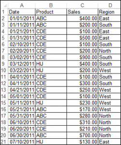
Pivot Tables are data summarization tools that you can use to draw key insights and summaries from your data. Let’s look at an example: we have a source data set in cells A1:D21 containing the details of products sold, shown below:
Using GetPivotData to Obtain a Value
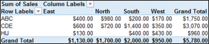
Assume you have a PivotTable called PivotTable1 with Sales in the Values/Data Field, Product as the Rows field and Region as the Columns field. You can use the PivotTable.GetPivotData method to return values from Pivot Tables.
The following code will return $1,130.00 (the total sales for the East Region) from the PivotTable:
MsgBox ActiveCell.PivotTable.GetPivotData("Sales", "Region", "East")
In this case, Sales is the “DataField”, “Field1” is the Region and “Item1” is East.
The following code will return $980 (the total sales for Product ABC in the North Region) from the Pivot Table:
MsgBox ActiveCell.PivotTable.GetPivotData("Sales", "Product", "ABC", "Region", "North")In this case, Sales is the “DataField”, “Field1” is Product, “Item1” is ABC, “Field2” is Region and “Item2” is North.
You can also include more than 2 fields.
The syntax for GetPivotData is:
GetPivotData (DataField, Field1, Item1, Field2, Item2…) where:
| Parameter | Description |
|---|---|
| Datafield | Data field such as sales, quantity etc. that contains numbers. |
| Field 1 | Name of a column or row field in the table. |
| Item 1 | Name of an item in Field 1 (Optional). |
| Field 2 | Name of a column or row field in the table (Optional). |
| Item 2 | Name of an item in Field 2 (Optional). |
Creating a Pivot Table on a Sheet
In order to create a Pivot Table based on the data range above, on cell J2 on Sheet1 of the Active workbook, we would use the following code:
Worksheets("Sheet1").Cells(1, 1).Select

ActiveWorkbook.PivotCaches.Create(SourceType:=xlDatabase, SourceData:= _

 "Sheet1!R1C1:R21C4", Version:=xlPivotTableVersion15).CreatePivotTable _

  TableDestination:="Sheet1!R2C10", TableName:="PivotTable1", DefaultVersion _

  :=xlPivotTableVersion15

  Sheets("Sheet1").Select
The result is:
Creating a Pivot Table on a New Sheet
In order to create a Pivot Table based on the data range above, on a new sheet, of the active workbook, we would use the following code:
Worksheets("Sheet1").Cells(1, 1).Select

Sheets.Add

    ActiveWorkbook.PivotCaches.Create(SourceType:=xlDatabase, SourceData:= _

 "Sheet1!R1C1:R21C4", Version:=xlPivotTableVersion15).CreatePivotTable _

  TableDestination:="Sheet2!R3C1", TableName:="PivotTable1", DefaultVersion _

  :=xlPivotTableVersion15

  Sheets("Sheet2").Select
Adding Fields to the Pivot Table
You can add fields to the newly created Pivot Table called PivotTable1 based on the data range above. Note: The sheet containing your Pivot Table, needs to be the Active Sheet.
To add Product to the Rows Field, you would use the following code:
ActiveSheet.PivotTables("PivotTable1").PivotFields("Product").Orientation = xlRowField

ActiveSheet.PivotTables("PivotTable1").PivotFields("Product").Position = 1
To add Region to the Columns Field, you would use the following code:
ActiveSheet.PivotTables("PivotTable1").PivotFields("Region").Orientation = xlColumnField

ActiveSheet.PivotTables("PivotTable1").PivotFields("Region").Position = 1
To add Sales to the Values Section with the currency number format, you would use the following code:
ActiveSheet.PivotTables("PivotTable1").AddDataField ActiveSheet.PivotTables( _

        "PivotTable1").PivotFields("Sales"), "Sum of Sales", xlSum

    With ActiveSheet.PivotTables("PivotTable1").PivotFields("Sum of Sales")

        .NumberFormat = "$#,##0.00"

End With
The result is:
Changing the Report Layout of the Pivot Table
You can change the Report Layout of your Pivot Table. The following code will change the Report Layout of your Pivot Table to Tabular Form:
ActiveSheet.PivotTables("PivotTable1").TableStyle2 = "PivotStyleLight18"Deleting a Pivot Table
You can delete a Pivot Table using VBA. The following code will delete the Pivot Table called PivotTable1 on the Active Sheet:
ActiveSheet.PivotTables("PivotTable1").PivotSelect "", xlDataAndLabel, True
Selection.ClearContents
VBA Coding Made Easy
Stop searching for VBA code online. Learn more about AutoMacro — A VBA Code Builder that allows beginners to code procedures from scratch with minimal coding knowledge and with many time-saving features for all users!

Learn More
Format all the Pivot Tables in a Workbook
You can format all the Pivot Tables in a Workbook using VBA. The following code uses a loop structure in order to loop through all the sheets of a workbook, and formats all the Pivot Tables in the workbook:
Sub FormattingAllThePivotTablesInAWorkbook()
Dim wks As Worksheet
Dim wb As Workbook
Set wb = ActiveWorkbook
Dim pt As PivotTable

For Each wks In wb.Sheets
For Each pt In wks.PivotTables
pt.TableStyle2 = "PivotStyleLight15"
Next pt
Next wks

End Sub
To learn more about how to use Loops in VBA click here.
Removing Fields of a Pivot Table
You can remove fields in a Pivot Table using VBA. The following code will remove the Product field in the Rows section from a Pivot Table named PivotTable1 in the Active Sheet:
ActiveSheet.PivotTables("PivotTable1").PivotFields("Product").Orientation = _
xlHidden
Creating a Filter
A Pivot Table called PivotTable1 has been created with Product in the Rows section, and Sales in the Values Section. You can also create a Filter for your Pivot Table using VBA. The following code will create a filter based on Region in the Filters section:
ActiveSheet.PivotTables("PivotTable1").PivotFields("Region").Orientation = xlPageField

ActiveSheet.PivotTables("PivotTable1").PivotFields("Region").Position = 1
To filter your Pivot Table based on a Single Report Item in this case the East region, you would use the following code:
ActiveSheet.PivotTables("PivotTable1").PivotFields("Region").ClearAllFilters

ActiveSheet.PivotTables("PivotTable1").PivotFields("Region").CurrentPage = _

"East"
Let’s say you wanted to filter your Pivot Table based on multiple regions, in this case East and North, you would use the following code:
ActiveSheet.PivotTables("PivotTable1").PivotFields("Region").Orientation = xlPageField

ActiveSheet.PivotTables("PivotTable1").PivotFields("Region").Position = 1

ActiveSheet.PivotTables("PivotTable1").PivotFields("Region"). _
EnableMultiplePageItems = True

With ActiveSheet.PivotTables("PivotTable1").PivotFields("Region")

.PivotItems("South").Visible = False

.PivotItems("West").Visible = False

End With
VBA Programming | Code Generator does work for you!
Refreshing Your Pivot Table
You can refresh your Pivot Table in VBA. You would use the following code in order to refresh a specific table called PivotTable1 in VBA:
ActiveSheet.PivotTables("PivotTable1").PivotCache.Refresh
The GETPIVOTDATA function extracts the data stored in a PivotTable report. You can use this function to retrieve data as long as it is visible in the pivot table.
The easiest way to understand how the Getpivotdata function works:
- Simply type «=» into a cell
- Click on the Pivot Table value that you want to return.
- Excel automatically inserts the Getpivotdata function into the active cell.
To extract data from a cell in a pivot table, we can enter a normal cell link in cell D14, for example=C6.The GetPivotData function will automatically generate the formula as shown in the below screenshot:
Syntax =GETPIVOTDATA(data_field,pivot_table,field,item,…)
Let’s understandarguments of this
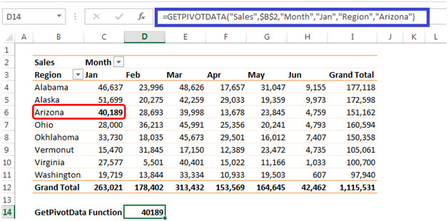
formula=GETPIVOTDATA(«Sales»,$B$2,»Month»,»Jan»,»Region»,»Arizona»)
- The first parameter is “Sales” which is the data_field from which we are extracting the numbers.
- The second argument is pivot_table in our example it is cell B2 from where our
PivotTable starts. - Fields are Month and Region.
- Items are Jan & Arizona.
Field & Items are entered as a pair & we can use a maximum as 126Arguments as shown in the below picture.
Using Cell References in GetPivotData
In a GetPivotData formula, refer to the pivot table, and the field(s) and item(s) that you want the data for. For example, this formula gets the Total, from the pivot table in D14, for the Month field, and the Washington item.
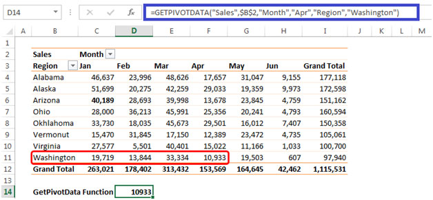
To make a GetPivotData formula more flexible, we can refer to worksheet cells, instead of typing the item or field names in the arguments.
Using the same example, we can enter “Apr” in cell L4 & “Washington” in cell L5. Then, change the formula in cell D14to reflect L4 & L5, instead of typing “Apr” & «Washington» in the formula.

Formula in cell D14 =GETPIVOTDATA(«Sales»,$B$2,»Month»,L4,»Region»,L5)
If you do not want to automatically generate the GetPivotData Function you can get rid of it by following the given steps:
- Click on any cell in the PivotTable
- Under PivotTable Tools contextual menu, go to the Analyze menu on the ribbon.

- Click on Pivot Table
- Under Options
- Click on Generate GetPivotData

Alternatively, Under File?Options?Click on Formulas de-select Use GetPivotData functions for PivotTable references. Click on Ok.

In this way we can extract data from pivot table.