
Excel for Microsoft 365 Excel for Microsoft 365 for Mac Excel for the web Excel 2021 Excel 2021 for Mac Excel 2019 Excel 2019 for Mac Excel 2016 Excel 2016 for Mac Excel 2013 More…Less
If you need a quick way to count rows that contain data, select all the cells in the first column of that data (it may not be column A). Just click the column header. The status bar, in the lower-right corner of your Excel window, will tell you the row count.
Do the same thing to count columns, but this time click the row selector at the left end of the row.
The status bar then displays a count, something like this:

If you select an entire row or column, Excel counts just the cells that contain data. If you select a block of cells, it counts the number of cells you selected. If the row or column you select contains only one cell with data, the status bar stays blank.
Notes:
-
If you need to count the characters in cells, see Count characters in cells.
-
If you want to know how many cells have data, see Use COUNTA to count cells that aren’t blank.
-
You can control the messages that appear in the status bar by right-clicking the status bar and clicking the item you want to see or remove. For more information, see Excel status bar options.
Need more help?
You can always ask an expert in the Excel Tech Community or get support in the Answers community.
Need more help?
Want more options?
Explore subscription benefits, browse training courses, learn how to secure your device, and more.
Communities help you ask and answer questions, give feedback, and hear from experts with rich knowledge.
How to Count the Number of Rows in Excel?
Here are the different ways of counting rows in Excel using the formula, rows with data, empty rows, rows with numerical values, rows with text values, and many other things related to counting the number of rows in Excel.
You can download this Count Rows Excel Template here – Count Rows Excel Template
Table of contents
- How to Count the Number of Rows in Excel?
- #1 – Excel Count Rows which has only the Data
- #2 – Count all the rows that have the data
- #3 – Count the rows that only have the numbers
- #4 – Count Rows, which only has the Blanks
- #5 – Count rows that only have text values
- #6 – Count all of the rows in the range
- Things to Remember
- Recommended Articles
#1 – Excel Count Rows which has only the Data
Firstly, we will see how to count the number of rows in Excel with the data. There could be empty rows between the data, but we often need to ignore them and find exactly how many rows contain the data in it.
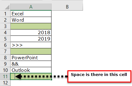
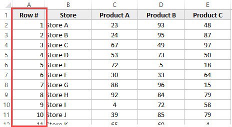
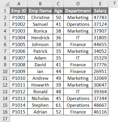
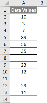
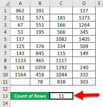
- We can count the number of rows with data by selecting the range of cells in Excel. For example, take a look at the below data.

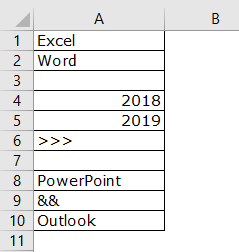
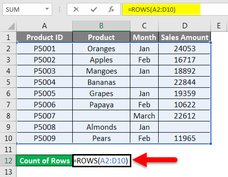
We have a total of 10 rows (border inserted area). In this 10 row, we want to count exactly how many cells have data. Since this is a small list of rows, we can easily calculate the number of rows. But when it comes to the huge database, it is impossible to count manually. So, this article will help you with this.
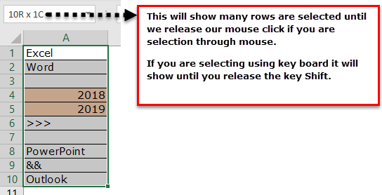
- Firstly, we must select all the rows in Excel.

- It is not telling us how many rows contain the data here. Instead, look at the Excel screen’s right-hand side bottom, i.e., a status bar.

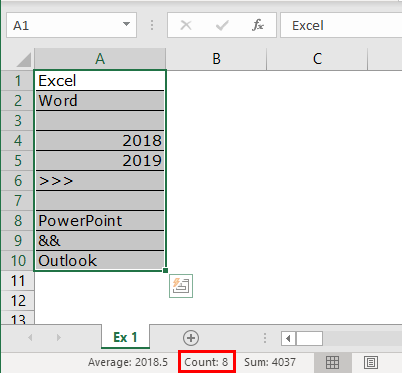
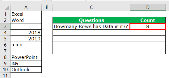
Take a look at the red circled area. It says COUNT as 8, which means that out of 10 selected rows, 8 have data.
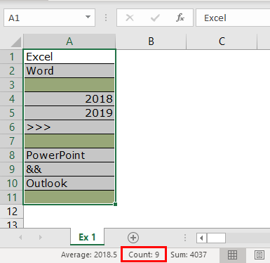
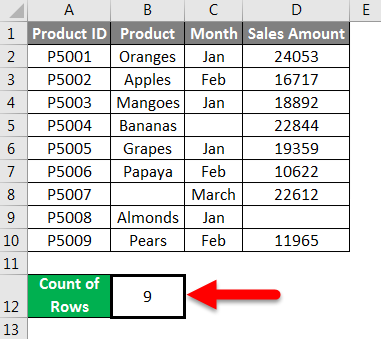
- Now, we will select one more row in the range and see what the count will be.

- We have selected 11 rows, but the count says 9, whereas we have data only in 8 rows. When we closely examine the cells, the 11th row contains a space.

Even though there is no value in the cell and it has only space Excel will be treated as the cell which contains the data.
#2 – Count all the rows that have the data
We know how to check how many rows contain the data quickly. But that is not the dynamic way of counting rows that have data. Instead, we need to apply the COUNTA function to count how many rows contain the data.
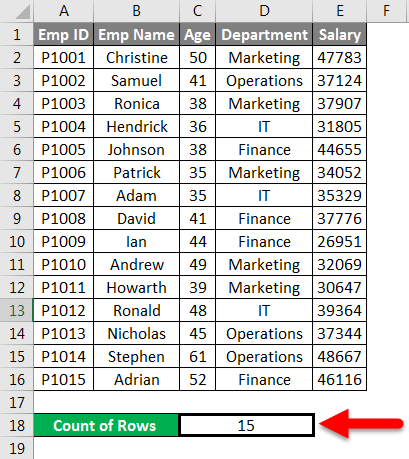
We will apply the COUNTA function in the D3 cell.
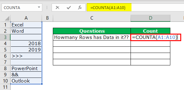
So, the total number of rows containing the data is 8 rows. Even this formula treats space as data.
#3 – Count the rows that only have the numbers
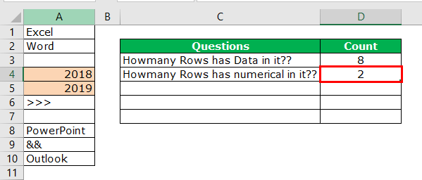
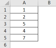
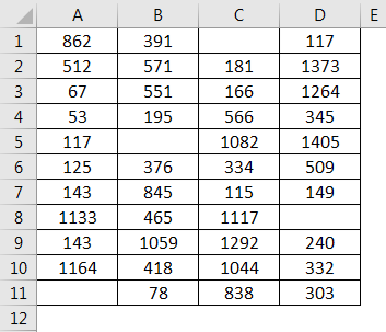
Here we want to count how many rows contain only numerical values.
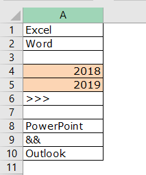
We can easily say 2 rows contain numerical values. Let us examine this by using a formula. We have a built-in formula called COUNT which counts only numerical values in the supplied range.
![]()
We will apply the COUNT function in cell B1 and select the range as A1 to A10.
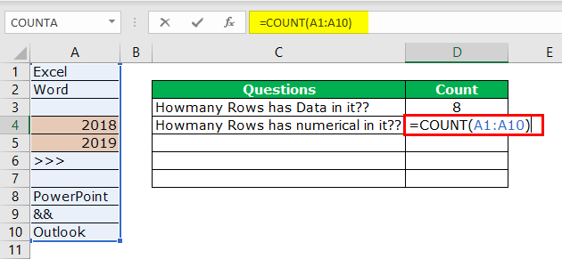
The COUNT function also says 2 as a result. So, out of 10 rows, only rows contain numerical values.
#4 – Count Rows, which only has the Blanks
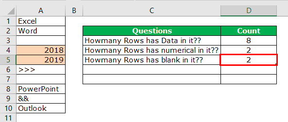
We can find only blank rows by using the COUNTBLANK function in Excel.
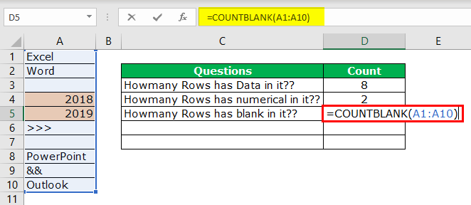
We have 2 blank rows in the selected range, which are revealed by the count blank function.
#5 – Count rows that only have text values
Remember, we do not have any straight in the COUNTTEXT function. Unlike in previous cases, we need to think differently here. We can use the COUNTIF functionThe COUNTIF function in Excel counts the number of cells within a range based on pre-defined criteria. It is used to count cells that include dates, numbers, or text. For example, COUNTIF(A1:A10,”Trump”) will count the number of cells within the range A1:A10 that contain the text “Trump”
read more with a wildcard character asterisk (*).
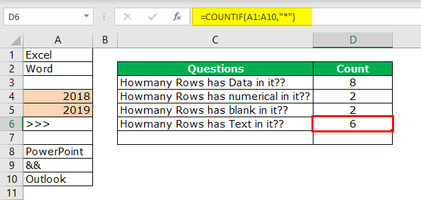
Here all the magic is done by the wildcard character asterisk (*). It matches any of the alphabets in the row and returns the result as a text value row. Even if the row contains numerical and text values, it will be treated as text value only.
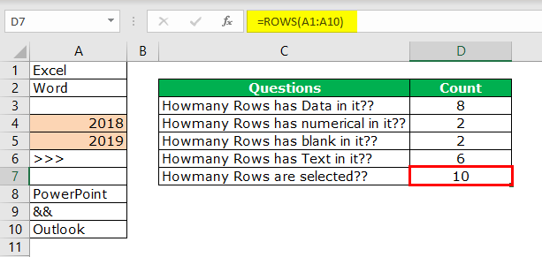
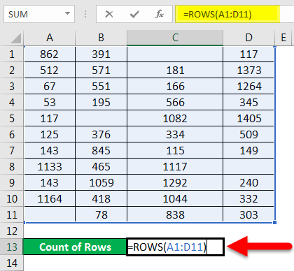
#6 – Count all of the rows in the range
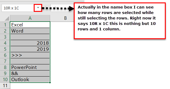
Now comes the important part. How do we count how many rows we have selected? One uses the Name Box in excel, which is limited while still choosing the rows. But how do we measure then?
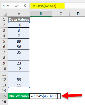
We have a built-in ROWS formula, which returns how many rows are selected.
Things to Remember
- Even space is treated as a value in the cell.
- If the cell contains numerical and text values, it will be treated as a text value.
- ROW may return the current row we are in, but ROWS will return how many are in the supplied range even though there is no data in the rows.
Recommended Articles
This article has been a guide to Count Rows in Excel. Here, we discuss the top 6 ways of counting rows in Excel using the formula: rows with data, empty rows, rows with numerical values, rows with text values, and many other things related to counting rows in Excel and practical examples and downloadable Excel templates. You may learn more about Excel from the following articles: –
- VBA COUNTIF
- Add Multiple Rows in Excel
- Excel Count Formula
- How to Insert Multiple Rows in Excel?
How to get the row or column number of the current cell or any other cell in Excel.
This tutorial covers important functions that allow you to do everything from alternate row and column shading to incrementing values at specified intervals and much more.
We will use the ROW and COLUMN function for this. Here is an example of the output from these functions.
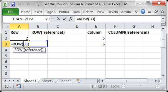
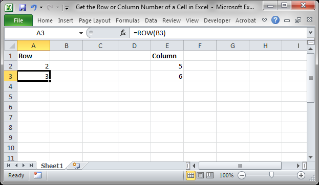
Though this doesn’t look like much, these functions allow for the creation of powerful formulas when combined with other functions. Now, let’s look at how to create them.
Get a Cell’s Row Number
Syntax
This function returns the number of the row that a particular cell is in.
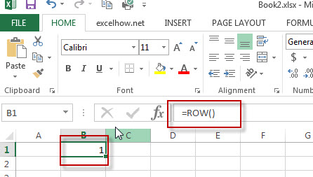
If you leave the function empty, it will return the row number for the current cell in which this function has been placed.
If you put a cell reference within this function, it will return the row number for that cell reference.
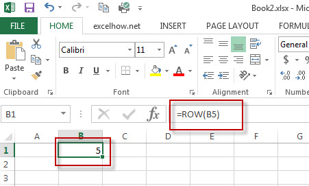
This example would return 1 since cell A1 is in row 1. If it was =ROW(C24) the function would return the number 24 because cell C24 is in row 24.
Examples
Now that you know how this function works, it may seem rather useless. Here are links to two examples where this function is key.
Increment a Value Every X Number of Rows in Excel
Shade Every Other Row in Excel Quickly
Get a Cell’s Column Number
Syntax
This function returns the number of the column that a particular cell is in. It counts from left to right, where A is 1 and B is 2 and so on.
If you leave the function empty, it will return the column number for the current cell in which this function has been placed.
If you put a cell reference within this function, it will return the column number for that cell reference.
This example would return 1 since cell A1 is in row 1. If it was =COLUMN (C24) the function would return the number 3 because cell C24 is in column number 3.
Examples
The COLUMN function works just like the ROW function does except that it works on columns, going left to right, whereas the ROW function works on rows, going up and down.
As such, almost every example where ROW is used could be converted to use COLUMN based on your needs.
Notes
The ROW and COLUMN functions are building blocks in that they help you create more complex formulas in Excel. Alone, these functions are pretty much worthless, but, if you can memorize them and keep them for later, you will start to find more and more uses for them when working in large data sets. The examples provided above in the ROW section cover only two of many different ways you can use these functions to create more powerful and helpful spreadsheets.
Similar Content on TeachExcel
Sum Values from Every X Number of Rows in Excel
Tutorial: Add values from every x number of rows in Excel. For instance, add together every other va…
Formulas to Remove First or Last Character from a Cell in Excel
Tutorial: Formulas that allow you to quickly and easily remove the first or last character from a ce…
Formula to Delete the First or Last Word from a Cell in Excel
Tutorial:
Excel formula to delete the first or last word from a cell.
You can copy and paste the fo…
Reverse the Contents of a Cell in Excel — UDF
Macro: Reverse cell contents with this free Excel UDF (user defined function). This will mir…
Excel Function to Remove All Text OR All Numbers from a Cell
Tutorial: How to create and use a function that removes all text or all numbers from a cell, whichev…
Get the First Word from a Cell in Excel
Tutorial: How to use a formula to get the first word from a cell in Excel. This works for a single c…
Subscribe for Weekly Tutorials
BONUS: subscribe now to download our Top Tutorials Ebook!
Summary
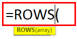
The Excel ROWS function returns the count of rows in a given reference. For example, ROWS(A1:A3) returns 3, since the range A1:A3 contains 3 rows.
Purpose
Get the number of rows in an array or reference.
Return value
Arguments
- array — A reference to a cell or range of cells.
Syntax
Usage notes
The ROWS function returns the count of rows in a given reference as a number. For example, =ROWS(A1:A5) returns 5, since the range A1:A5 contains 5 rows. ROWS takes just one argument, called array, which can be a range or array.
Examples
Use the ROWS function to get the row count for a given reference or range. For example, there are 10 rows in the range A1:F10 so the formula below returns 10:
=ROWS(A1:F10) // returns 10
The range A1:Z100 contains 100 rows, so the formula below returns 100:
=ROWS(A1:Z100) // returns 100
You can also use the ROWS function to get a row count for an array constant:
=ROWS({1;2;3;4;5}) // returns 5
Although there is no built-in function to count the number of cells in a range, you can use the ROWS function together with the COLUMNS function like this:
=COLUMNS(range)*ROWS(range) // total cells
=COLUMNS(A1:Z100)*ROWS(A1:Z100) // returns 2600
More details here.
Notes
- Array can be a range or a reference to a single contiguous group of cells.
- Array can be an array constant or an array created by another formula.
- To count columns, see the COLUMNS function.
- To get row numbers, see the ROW function.
- To lookup a row number, see the MATCH function.

Author![]()
Dave Bruns
Hi — I’m Dave Bruns, and I run Exceljet with my wife, Lisa. Our goal is to help you work faster in Excel. We create short videos, and clear examples of formulas, functions, pivot tables, conditional formatting, and charts.
There are hundreds and hundreds of Excel sites out there. I’ve been to many and most are an exercise in frustration. Found yours today and wanted to let you know that it might be the simplest and easiest site that will get me where I want to go.
Get Training
Quick, clean, and to the point training
Learn Excel with high quality video training. Our videos are quick, clean, and to the point, so you can learn Excel in less time, and easily review key topics when needed. Each video comes with its own practice worksheet.
View Paid Training & Bundles
Help us improve Exceljet
In this article, we will learn about how to Count table rows & columns in Excel.
In simple words, while working with large data in Excel we need to find the number of rows or columns in excel table.
The ROWS function in excel returns the number of rows in an array.
Syntax:
The COLUMNS function in excel returns the number of columns in an array.
Syntax:
Let’s understand this function using it in an example.
Here we have large data A2:H245 named Sales_Data
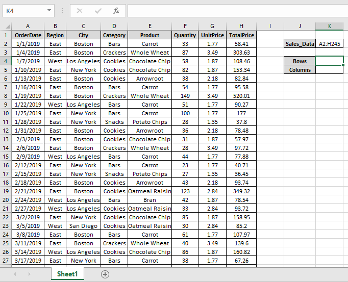
Here we need to find out the number of rows & columns of Sales_Data table in Excel.
Use the formula to get the number of rows
A2:H245 : Sales_Data table as an array.
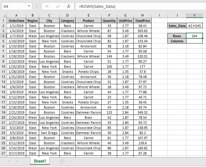
We got the number of rows of the Sales_Data.
Use the formula to get the number of rows
A2:H245 : Sales_Data table as an array.
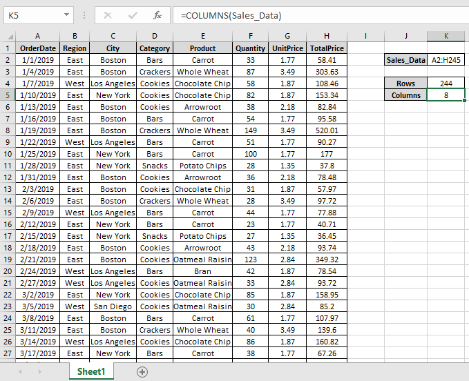
As you can see the ROWS & COLUMNS functions returns the number of rows & columns of table.
Hope you understood how to use ROWS function and COLUMNS function in Excel. Explore more articles on Excel cell info function functions here. Please feel free to state your query or feedback for the above article.
Related Articles :
How to use the CELL function in Excel
How to use the ROW function in Excel
How to use the COLUMN Function in Excel
Popular Articles :
50 Excel Shortcut to Increase Your Productivity : Get faster at your task. These 50 shortcuts will make you work even faster on Excel.
How to use the VLOOKUP Function in Excel : This is one of the most used and popular functions of excel that is used to lookup value from different ranges and sheets.
How to use the COUNTIF function in Excel : Count values with conditions using this amazing function. You don’t need to filter your data to count specific values. Countif function is essential to prepare your dashboard.
How to use the SUMIF Function in Excel : This is another dashboard essential function. This helps you sum up values on specific conditions.
Watch Video – 7 Quick and Easy Ways to Number Rows in Excel
When working with Excel, there are some small tasks that need to be done quite often. Knowing the ‘right way’ can save you a great deal of time.
One such simple (yet often needed) task is to number the rows of a dataset in Excel (also called the serial numbers in a dataset).
Now if you’re thinking that one of the ways is to simply enter these serial number manually, well – you’re right!
But that’s not the best way to do it.
Imagine having hundreds or thousands of rows for which you need to enter the row number. It would be tedious – and completely unnecessary.
There are many ways to number rows in Excel, and in this tutorial, I am going to share some of the ways that I recommend and often use.
Of course, there would be more, and I will be waiting – with a coffee – in the comments area to hear from you about it.
How to Number Rows in Excel
The best way to number the rows in Excel would depend on the kind of data set that you have.
For example, you may have a continuous data set that starts from row 1, or a dataset that start from a different row. Or, you might have a dataset that has a few blank rows in it, and you only want to number the rows that are filled.
You can choose any one of the methods that work based on your dataset.
1] Using Fill Handle
Fill handle identifies a pattern from a few filled cells and can easily be used to quickly fill the entire column.
Suppose you have a dataset as shown below:

Here are the steps to quickly number the rows using the fill handle:
Note that Fill Handle automatically identifies the pattern and fill the remaining cells with that pattern. In this case, the pattern was that the numbers were getting incrementing by 1.
In case you have a blank row in the dataset, fill handle would only work till the last contiguous non-blank row.
Also, note that in case you don’t have data in the adjacent column, double-clicking the fill handle would not work. You can, however, place the cursor on the fill handle, hold the right mouse key and drag down. It will fill the cells covered by the cursor dragging.
2] Using Fill Series
While Fill Handle is a quick way to number rows in Excel, Fill Series gives you a lot more control over how the numbers are entered.
Suppose you have a dataset as shown below:
Here are the steps to use Fill Series to number rows in Excel:
This will instantly number the rows from 1 to 26.
Using ‘Fill Series’ can be useful when you’re starting by entering the row numbers. Unlike Fill Handle, it doesn’t require the adjacent columns to be filled already.
Even if you have nothing on the worksheet, Fill Series would still work.
Note: In case you have blank rows in the middle of the dataset, Fill Series would still fill the number for that row.
3] Using the ROW Function
You can also use Excel functions to number the rows in Excel.
In the Fill Handle and Fill Series methods above, the serial number inserted is a static value. This means that if you move the row (or cut and paste it somewhere else in the dataset), the row numbering will not change accordingly.
This shortcoming can be tackled using formulas in Excel.
You can use the ROW function to get the row numbering in Excel.
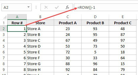
To get the row numbering using the ROW function, enter the following formula in the first cell and copy for all the other cells:
=ROW()-1
The ROW() function gives the row number of the current row. So I have subtracted 1 from it as I started from the second row onwards. If your data starts from the 5th row, you need to use the formula =ROW()-4.
The best part about using the ROW function is that it will not screw up the numberings if you delete a row in your dataset.
Since the ROW function is not referencing any cell, it will automatically (or should I say AutoMagically) adjust to give you the correct row number. Something as shown below:

Note that as soon as I delete a row, the row numbers automatically update.
Again, this would not take into account any blank records in the dataset. In case you have blank rows, it will still show the row number.
You can use the following formula to hide the row number for blank rows, but it would still not adjust the row numbers (such that the next row number is assigned to the next filled row).
IF(ISBLANK(B2),"",ROW()-1)
4] Using the COUNTA Function
If you want to number rows in a way that only the ones that are filled get a serial number, then this method is the way to go.
It uses the COUNTA function that counts the number of cells in a range that are not empty.
Suppose you have a dataset as shown below:
Note that there are blank rows in the above-shown dataset.
Here is the formula that will number the rows without numbering the blank rows.
=IF(ISBLANK(B2),"",COUNTA($B$2:B2))
The IF function checks whether the adjacent cell in column B is empty or not. If it’s empty, it returns a blank, but if it’s not, it returns the count of all the filled cells till that cell.
5] Using SUBTOTAL For Filtered Data
Sometimes, you may have a huge dataset, where you want to filter the data and then copy and paste the filtered data into a separate sheet.
If you use any of the methods shown above so far, you will notice that the row numbers remain the same. This means that when you copy the filtered data, you will have to update the row numbering.
In such cases, the SUBTOTAL function can automatically update the row numbers. Even when you filter the data set, the row numbers will remain intact.
Let me show you exactly how it works with an example.
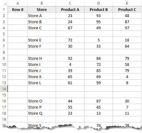
Suppose you have a dataset as shown below:

If I filter this data based on Product A sales, you will get something as shown below:

Note that the serial numbers in Column A are also filtered. So now, you only see the numbers for the rows that are visible.
While this is the expected behavior, in case you want to get a serial row numbering – so that you can simply copy and paste this data somewhere else – you can use the SUBTOTAL function.
Here is the SUBTOTAL function that will make sure that even the filtered data has continuous row numbering.
=SUBTOTAL(3,$B$2:B2)
The 3 in the SUBTOTAL function specifies using the COUNTA function. The second argument is the range on which COUNTA function is applied.
The benefit of the SUBTOTAL function is that it dynamically updates when you filter the data (as shown below):

Note that even when the data is filtered, the row numbering update and remains continuous.
6] Creating an Excel Table
Excel Table is a great tool that you must use when working with tabular data. It makes managing and using data a lot easier.
This is also my favorite method among all the techniques shown in this tutorial.
Let me first show you the right way to number the rows using an Excel Table:
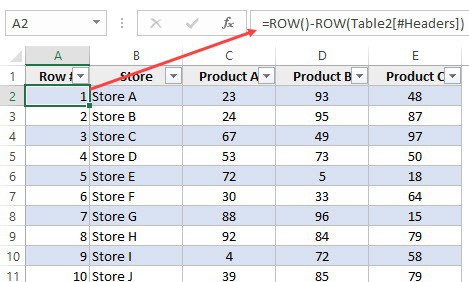
Note that in the formula above, I have used Table2, as that is the name of my Excel table. You can replace Table2 with the name of the table you have.
There are some added benefits of using an Excel Table while numbering rows in Excel:
- Since Excel Table automatically inserts the formula in the entire column, it works when you insert a new row in the Table. This means that when you insert/delete rows in an Excel Table, the row numbering would automatically update (as shown below).

- If you add more rows to the data, Excel Table would automatically expand to include this data as a part of the table. And since the formulas automatically update in the calculated columns, it would insert the row number for the newly inserted row (as shown below).


7] Adding 1 to the Previous Row Number
This is a simple method that works.
The idea is to add 1 to the previous row number (the number in the cell above). This will make sure that subsequent rows get a number that is incremented by 1.
Suppose you have a dataset as shown below:
Here are the steps to enter row numbers using this method:
- In the cell in the first row, enter 1 manually. In this case, it’s in cell A2.
- In cell A3, enter the formula, =A2+1
- Copy and paste the formula for all the cells in the column.

The above steps would enter serial numbers in all the cells in the column. In case there are any blank rows, this would still insert the row number for it.
Also note that in case you insert a new row, the row number would not update. In case you delete a row, all the cells below the deleted row would show a reference error.
These are some quick ways you can use to insert serial numbers in tabular data in Excel.
In case you are using any other method, do share it with me in the comments section.
You May Also Like the Following Excel Tutorials:
- Delete Blank Rows in Excel (with and without VBA).
- How to Insert Multiple Rows in Excel (4 Methods).
- How to Split Multiple Lines in a Cell into a Separate Cells / Columns.
- 7 Amazing Things Excel Text to Columns Can Do For You.
- Highlight EVERY Other ROW in Excel.
- How to Compare Two Columns in Excel.
- Insert New Columns in Excel

Excel Row Count (Table of Contents)
- Introduction to Row Count in Excel
- How to Count the Rows in Excel?
Introduction to Row Count in Excel
Excel provides many built-in functions through which we can do multiple calculations. We can also count the rows and columns in Excel. Here in this article, we will discuss the Row Count in Excel. If we want to measure the rows which contain data, select all the cells of the first column by clicking on the column header. It will display the row count on the status bar in the lower right corner.
Let’s take some values in the Excel sheet.
Select the entire column which contains data. Now click on the column label for counting the rows; it will show you the row count. Refer to the below screenshot:

There are two types of functions for counting the rows.
- ROW()
- ROWS()
The ROW() function gives you the row number of a particular cell.
The ROWS() function gives you the count of rows in a range.
How to Count the Rows in Excel?
Let’s take some examples to understand the usage of ROWS functions.
You can download this Row Count Excel Template here – Row Count Excel Template
Example #1
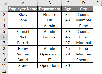
We have given the below employee data.
For counting the rows here, we will use the below function here:
=ROWS(range)
Where range = a range of cells containing data.
Now we will apply the above function like the below screenshot:

Which returns the number of rows containing the data in the supplied range.
The final result is given below:
Example #2
We have given below some student marks subject-wise.
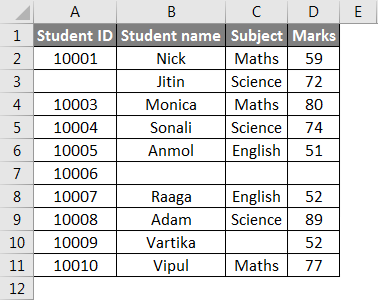
As we can see in the above dataset, certain information is absent.
As per the screenshot below, we will apply the ROWS function for counting the rows containing data.
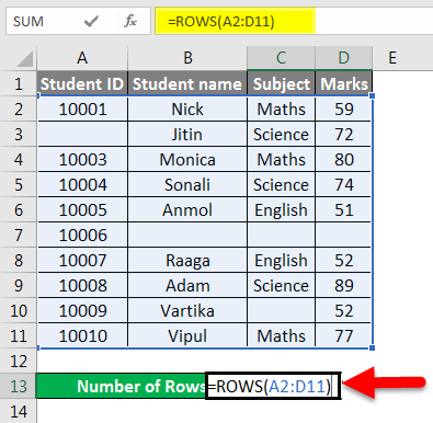
The final result is given below:

Example #3
We have given the below data values.
We will pass the range of data values within the function for counting the number of rows.
Apply the function like the below screenshot:
Press ENTER key here, and it will return the count of rows.
The final result is shown below:
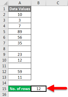
Explanation:
When we pass the range of cells, it gives you the count of cells you selected.
Example #4
We have given below product details:
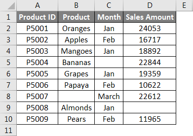
Now we will pass the range of the given dataset within the function like the below screenshot:
Press ENTER key, which will give you the count of rows containing data in the passing range.
The final result is given below:
Example #5
We have given some raw data.
Some cell values are missing here, so now, for counting the rows, we will apply the function shown in the below screenshot:
Hit the Enter key, and it will return the count of rows having data.
The final result is given below:
Example #6
We have given a company employee data where some details are missing:
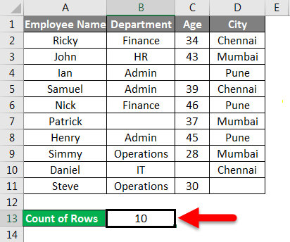
Now apply the ROWS function to count the row containing data of employees:
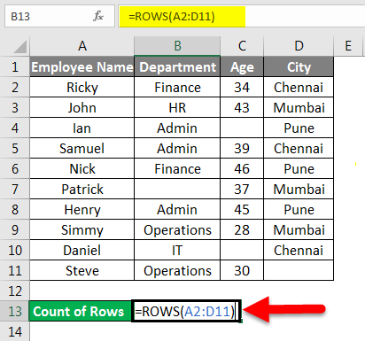
Hit the Enter key to get the final rows
Things to Remember About Row Count in Excel
- When you click on the column heading for counting the rows, it will give you the count which contains data.
- If you pass a range of cells, it will return the number of cells that you have selected.
- The status bar won’t show you anything if the column contains the data only in one cell. That is, the status bar stays blank.
- If the data are given in the table form, then for counting the rows, you can pass the table range within the ROWS function.
- You can also do the setting of the message in the status bar. Do right-click on the status bar and click the item you want to see or remove.
Recommended Articles
This article has been a guide to Row Count in Excel. Here we discussed How to Count the Rows, practical examples, and a downloadable Excel template. You can also go through our other suggested articles–
- COUNTA Function in Excel
- Count Function in Excel
- ROWS Function in Excel
- Add Rows in Excel Shortcut
This post will guide you how to use Excel ROW function with syntax and examples in Microsoft excel.
Table of Contents
- Description
- Syntax
- Excel Row Function Examples
- Related Functions
- More Excel ROW Formula Examples
Description
The Excel ROW function returns the row number of a cell reference.
The ROW function is a build-in function in Microsoft Excel and it is categorized as a Lookup and Reference Function.
The ROW function is available in Excel 2016, Excel 2013, Excel 2010, Excel 2007, Excel 2003, Excel XP, Excel 2000, Excel 2011 for Mac.
Syntax
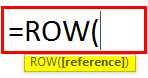
The syntax of the ROW function is as below:
= ROW ([reference])
Where the ROW function arguments is:
Reference – This is an Optional argument. the cell or range of cells reference that you want to get the row number.
Note: If the reference is omitted, the ROW function will return the row number of the current cell.
Excel Row Function Examples
The below examples will show you how to use Excel ROW Lookup and Reference Function to return the row number of a cell reference.
#1 To get the row number of “B5” cell in B1 Cell, just using the following excel formula: =ROW(B5)
#2 To get the row number of the current cell, just using excel formula: =ROW()
#3 get the first row number of range in excel
You can get the first row number in a range with an excel formula based on the ROW function as follows:
=ROW(Range)
=MIN(ROW(Range))
The ROW function will only display the first row number.
- Excel MIN function
The Excel MIN function returns the smallest numeric value from the numbers that you provided. Or returns the smallest value in the array.The MIN function is a build-in function in Microsoft Excel and it is categorized as a Statistical Function.The syntax of the MIN function is as below:= MIN(num1,[num2,…numn])….
More Excel ROW Formula Examples
- Get the Position of the nth Occurrence of a Character in a Cell
If you want to get the position of the nth occurrence of a character using a excel formula, you can use the FIND function in combination with the SUBSTITUTE function. - Get the position of Last Occurrence of a character or string in a cell
If you want to get the position of the last occurrence of a character in a cell, then you can use a combination of the LOOKUP function, the MID function, the ROW function, the INDIRECT function and the LEN function to create an excel formula.… - Find the Relative Position in a Range or Table
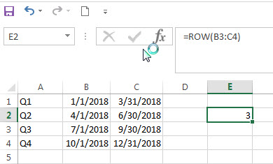
If you want to know the relative row position for all rows in an Excel Range (B3:D6), you can use a excel Array formula as follows:=ROW(B3:D6)- ROW(B3) + 1. You can also use another excel array formula to get the same result as follows:=ROW(B3:D6)-ROW(INDEX(B3:D6,1,1))+1… - Get the First Row Number in a Range
If the ROW function use a Range as its argument, it only returns the first row number.You can also use the ROW function within the MIN function to get the first row number in a range. You can also use the INDEX function to get the reference of the first row in a range, then combined to the ROW function to get the first row number of a range.… - Get the Last Row Number in a Range
If you want to get the last row number in a range, you need to know the first row number and the total rows number of a range, then perform the addition operation, then subtract 1, the last result is the last row number for that range.… - Get the position of Last Occurrence of a value in a column
If you want to find the position number of the last occurrence of a specific value in a column (a single range), you can use an array formula with a combination of the MAX function, IF function, ROW function and INDEX Function. - Get the position of nth occurrence of a value in column
If you want to locate the second, third or nth occurrence of a specified value, you can use a combination of the INDEX function, the IF function, ROW function and SMALL function to create a new excel array formula. - Split Text String to an Array
If you want to convert a text string into an array that split each character in text as an element, you can use an excel formula to achieve this result. the below will guide you how to use a combination of the MID function, the ROW function, the INDIRECT function and the LEN function to split a string… - Three Ways to Get the Last Row Number in a Range
If you want to get the last row number in a range, you need to know the first row number and the total rows number of a range, then perform the addition operation, then subtract 1, the last result is the last row number for that range… - Three Ways to get the First Row Number in a Range
you can use ROW function to get the first row number in a range directly. You can also use the ROW function within the MIN function to get the first row number in a range.You can also use the INDEX function to get the reference of the first row in a range, then combined to the ROW function to get the first row number of a range… - Transpose Multiple Columns into One Column
You can use the following excel formula to transpose multiple columns that contain a range of data into a single column, and you can also write an Excel VBA Macro to transpose the data of range in B1:D4 into single column F quickly… - Delete Every Other Row
To delete every other row in Excel, you need to filter alternate rows, and then select those rows, and delete them at once. So you need to create a helper column using MOD function with ROW function… - Sum Numbers from 1 to N
Assuming that you supply a number 100, and you want to sum the numbers from 1 to 100 (1+2+3+…+100), you need to create a formula based on the SUMPRODUCT function, the ROW function and the INDIRECT function to achieve the result..…. - Split Data in One Column to Multiple Columns
If you want to split each sets in one column from row to row in stacked columns, and you need to create a formula based on the OFFSET function, the COLUMNS function, and the ROWS function..… - VLOOKUP Return Multiple Values Horizontally
You can create a complex array formula based on the INDEX function, the SMALL function, the IF function, the ROW function and the COLUMN function to vlookup a value and then return multiple corresponding values horizontally in Excel.… - Copy and Paste Only Non-blank Cells
If you want only copy non-blank cells in a range in Excel, you need to select the non-blank cells firstly, then press Ctrl +C keys to copy the selected cells. So how to only select all non-blank cells in the selected range in your worksheet..… - Sum Every Nth Row or Column
If you want to sum every nth rows in Excel, you can create an Excel Array formula based on the SUM function, the MOD function and the ROW function..…. - Generate All Possible Combinations of Two Lists
You can use a formula based on the IF function, the ROW function, the COUNTA function, The INDEX function and the MOD function to get a list of all possible combinations from those two list…. - Find Missing Numbers in a Sequence in Excel
You can use an excel array formula based on the SMALL function, the IF function, the ISNA function, the MATCH function, and the ROW function to find missing numbers in a sequence…