
Excel for Microsoft 365 Excel for Microsoft 365 for Mac Excel for the web Excel 2021 Excel 2021 for Mac Excel 2019 Excel 2019 for Mac Excel 2016 Excel 2016 for Mac Excel 2013 More…Less
If you need a quick way to count rows that contain data, select all the cells in the first column of that data (it may not be column A). Just click the column header. The status bar, in the lower-right corner of your Excel window, will tell you the row count.
Do the same thing to count columns, but this time click the row selector at the left end of the row.
The status bar then displays a count, something like this:

If you select an entire row or column, Excel counts just the cells that contain data. If you select a block of cells, it counts the number of cells you selected. If the row or column you select contains only one cell with data, the status bar stays blank.
Notes:
-
If you need to count the characters in cells, see Count characters in cells.
-
If you want to know how many cells have data, see Use COUNTA to count cells that aren’t blank.
-
You can control the messages that appear in the status bar by right-clicking the status bar and clicking the item you want to see or remove. For more information, see Excel status bar options.
Need more help?
You can always ask an expert in the Excel Tech Community or get support in the Answers community.
Need more help?
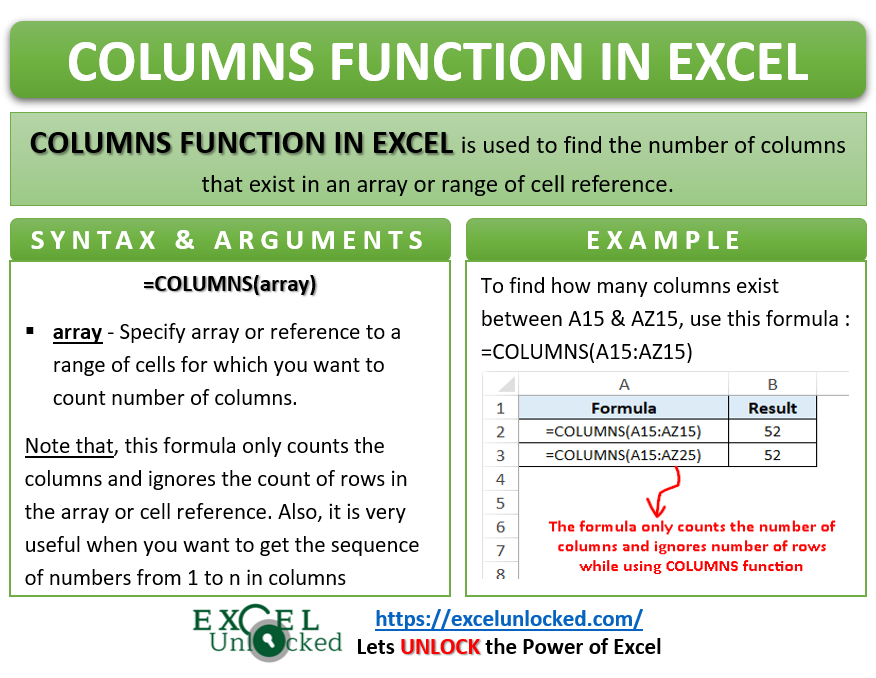
In this article, we will learn about how to Count table rows & columns in Excel.
In simple words, while working with large data in Excel we need to find the number of rows or columns in excel table.
The ROWS function in excel returns the number of rows in an array.
Syntax:
The COLUMNS function in excel returns the number of columns in an array.
Syntax:
Let’s understand this function using it in an example.
Here we have large data A2:H245 named Sales_Data
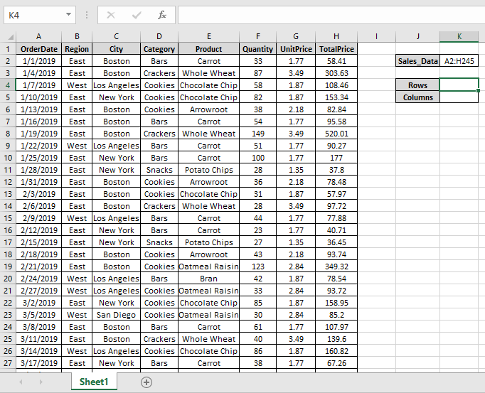
Here we need to find out the number of rows & columns of Sales_Data table in Excel.
Use the formula to get the number of rows
A2:H245 : Sales_Data table as an array.
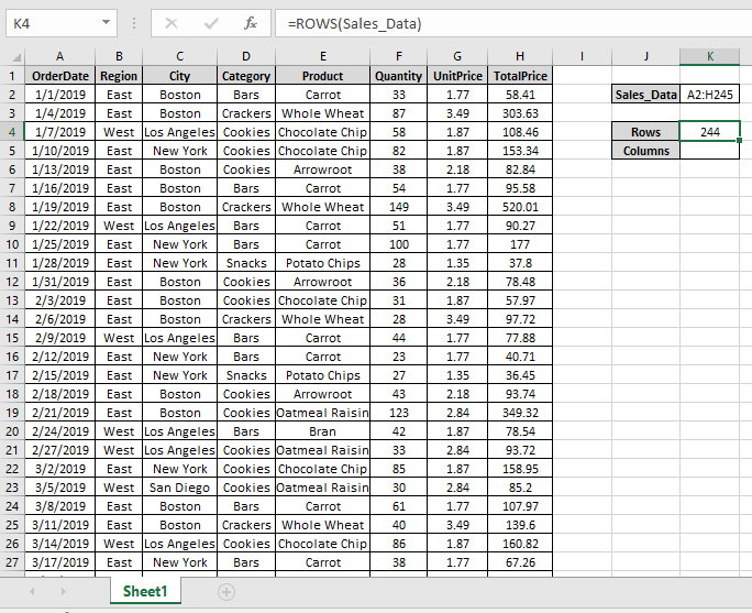
We got the number of rows of the Sales_Data.
Use the formula to get the number of rows
A2:H245 : Sales_Data table as an array.
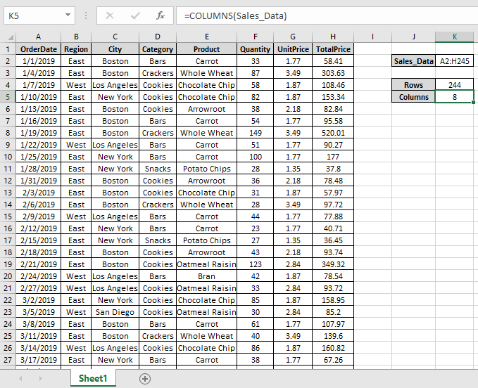
As you can see the ROWS & COLUMNS functions returns the number of rows & columns of table.
Hope you understood how to use ROWS function and COLUMNS function in Excel. Explore more articles on Excel cell info function functions here. Please feel free to state your query or feedback for the above article.
Related Articles :
How to use the CELL function in Excel
How to use the ROW function in Excel
How to use the COLUMN Function in Excel
Popular Articles :
50 Excel Shortcut to Increase Your Productivity : Get faster at your task. These 50 shortcuts will make you work even faster on Excel.
How to use the VLOOKUP Function in Excel : This is one of the most used and popular functions of excel that is used to lookup value from different ranges and sheets.
How to use the COUNTIF function in Excel : Count values with conditions using this amazing function. You don’t need to filter your data to count specific values. Countif function is essential to prepare your dashboard.
How to use the SUMIF Function in Excel : This is another dashboard essential function. This helps you sum up values on specific conditions.
Summary
The Excel COLUMNS function returns the count of columns in a given reference. For example, COLUMNS(A1:C3) returns 3, since the range A1:C3 contains 3 columns.
Purpose
Get the number of columns in an array or reference.
Return value
Arguments
- array — A reference to a range of cells.
Syntax
Usage notes
The COLUMNS function returns the count of columns in a given reference as a number. For example, COLUMNS(A1:C3) returns 3, since the range A1:C3 contains 3 columns. COLUMNS takes just one argument, called array, which should be a range or array.
Examples
Use the COLUMNS function to get the column count for a given reference or range. For example, there are 6 columns in the range A1:F1 so the formula below returns 6:
=COLUMNS(A1:F1) // returns 6
The range A1:Z100 contains 26 columns, so the formula below returns 100:
=COLUMNS(A1:Z100) // returns 26
You can also use the COLUMNS function to get a column count for an array constant:
=COLUMNS({1,2,3,4,5}) // returns 5
Although there is no built-in function to count the number of cells in a range, you can use the COLUMNS function together with the ROWS function like this:
=COLUMNS(range)*ROWS(range) // total cells
=COLUMNS(A1:Z100)*ROWS(A1:Z100) // returns 2600
More details here.
Notes
- Array can be a range or a reference to a single contiguous group of cells.
- Array can be an array constant or an array created by another formula.
- To count rows, see the ROW function.
- To get column numbers, see the COLUMN function.
- To lookup a column number, see the MATCH function.

Author![]()
Dave Bruns
Hi — I’m Dave Bruns, and I run Exceljet with my wife, Lisa. Our goal is to help you work faster in Excel. We create short videos, and clear examples of formulas, functions, pivot tables, conditional formatting, and charts.
Excel COLUMNS Function (Example + Video)

When to use Excel COLUMNS Function
Excel COLUMNS function can be used when you want to get the number of columns in a specified range or array.
What it Returns
It returns a number that represents the total number of columns in the specified range or array.
Syntax
=COLUMNS(array)
Input Arguments
- array – it could be an array, an array formula or a reference to a contiguous range of cells.
Additional Notes
- Even if the array contains multiple rows and columns, only the columns are counted. For example:
-
COLUMNS(A1:B1) returns 2.
-
COLUMNS(A1:B100) also returns 2.
-
- This formula can be useful when you want to get a sequence of numbers as you go to the right in your worksheet.
- For example, if you want 1 in A1, 2 in B1, 3 in C1 and so on, use the following formula =COLUMNS($A$1:A1). As you would drag this to the right, the reference inside it would change and the number of columns in the reference would get incremented by one. For example, when you drag it to column B1, the formula becomes COLUMNS($A$1:B1) which then returns 2.
Excel COLUMNS Function – Examples
Here are two examples of using the Excel COLUMNS function.
Example 1: Finding the number of Columns in an Array

In the example above, =COLUMNS(A1:A1) returns 1 as it covers one row (which is A1). Similarly, =COLUMNS(A1:C1) returns 3 as the array A1:C1 covers four columns in it.
Also, note that it only counts the number of columns. Hence, whether the array is A1:C1, or A1:C5, it would return 3 in both the cases.
Example 2: Getting a Sequence of Numbers in a Column

Excel COLUMNS function can be used to get a sequence of numbers. Since the first reference is fixed, as you copy the formula down, the second reference changes and so does the row numbers in the array.
Excel COLUMNS Function – Video Tutorial
Related Excel Functions:
- Excel COLUMN Function.
- Excel ROW Function.
- Excel ROWS Function
Other articles you may also like:
- Row vs Column in Excel – What’s the Difference?
In this tutorial, we would unlock one of the reference functions called the COLUMNS function in Excel. The excel reference functions are nothing but those excel formulas which return a reference of the cell.
This blog covers the use of COLUMNS excel formula, function syntax and arguments, and its examples.
When to Use Excel COLUMNS Formula
The COLUMNS formula in excel is used to find the number of columns within an array or range of cells. It means it helps to return or get the count of columns in a range of cells or array.
The result of this formula is a whole number (1, 2, 3, 4, … and so on).
Syntax and Argument
=COLUMNS(array)
As seen above, the COLUMNS excel formula in contains one argument which is ‘array’.
- array – In this argument, specify the array or a reference to a range of cells.
Let us consider one very basic example of the COLUMNS formula. Finding number of columns between two cells becomes very easy with this formula.
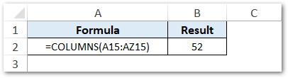
Suppose you want to count how many columns exist between two cells (A15 and AZ15). In that case, use the below formula:
=COLUMNS(A15:AZ15)
As a result, you would notice that excel returns the count of columns between these excel cell references. The result comes to 52, meaning there are in total 52 columns in between these two cell references.
Do Not Miss These Points
Below are some important points that you need to consider while using the COLUMNS function in Excel-
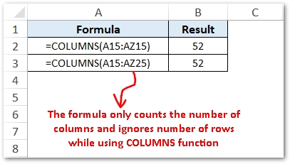
- This formula only counts the columns and ignores the count of rows in the array or cell reference. For example, =COLUMNS(A15:AZ15) and =COLUMNS(A15:AZ25) both the formulas would return 52 as output.
- This formula is very useful when you want to get the sequence of numbers from 1 to n in columns something like this:
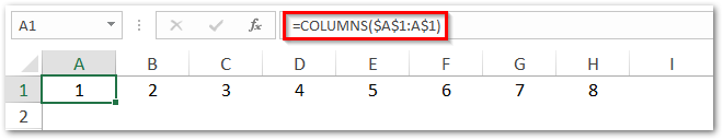
- In the above image, we have used the formula =COLUMNS($A$1:A$1) to return the number of columns between $A$1 and A$1 in cell A1. We have then copied this formula to other columns (B, C, D … and so on). By keeping A as a non-absolute reference in A$1, excel increments to B, C, D, and so on as you copy it to other columns B1, C1, etc.
RELATED POSTS
-
CELL Function in Excel – Get Information About Cell
-
Excel COUNT Function – Count Cell Containing Numbers
-
ADDRESS Function in Excel – Get Excel Cell Address
-
ROW Function in Excel – Get Cell Row Number
-
SEQUENCE Function in Excel – Generate Number Series
-
AREAS Function in Excel – Areas of Reference
Excel allows a user to count table columns, using the COLUMNS function. This step by step tutorial will assist all levels of Excel users in counting table columns.
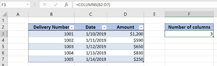 Figure 1. The result of the formula
Syntax of the Formula
The generic formula is:
=COLUMNS(array)
The parameter of the COLUMNS function is:
- array – an array of cells in a table for which we want to count columns or a table name.
Setting up Our Data for the Example
Let’s look at the structure of the data we will use. In column B, we have the price and in column C, we have the cost. In column D, we want to calculate a profit margin percentage.
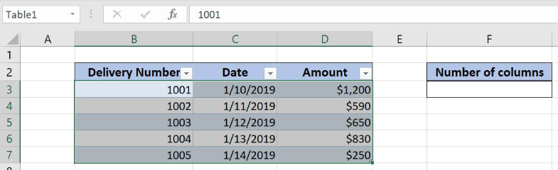 Figure 2. Data that we will use in the example
Counting a Table Columns with a Range
In the first example, we want to count columns in the Excel table, using the table range.
The formula looks like:
=COLUMNS(B2:D7)
The parameter array is the range B2:D7.
To apply the formula, we need to follow these steps:
- Select cell F3 and click on it
- Insert the formula:
=COLUMNS(B2:D7) - Press enter
 Figure 3. Counting the table columns with the range
The result in the cell D3 is 3, as there are 3 columns in the table.
Counting a Table Columns with a Table Name
In this example, we want to count the number of columns in the table, using the table name. The table in the range B2:D7 has name “Table1”.
The formula looks like:
=COLUMNS(Table1)
The parameter array is the range Table1.
To apply the formula, we need to follow these steps:
- Select cell F3 and click on it
- Insert the formula:
=COLUMNS(Table1) - Press enter
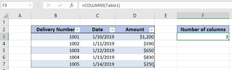 Figure 4. Counting the table columns with the table name
As we can see in Figure 4, the result in the cell D3 is 3, the same as in the previous example.
Most of the time, the problem you will need to solve will be more complex than a simple application of a formula or function. If you want to save hours of research and frustration, try our live Excelchat service! Our Excel Experts are available 24/7 to answer any Excel question you may have. We guarantee a connection within 30 seconds and a customized solution within 20 minutes.
The COLUMNS function is a built-in function in Microsoft Excel. It falls under the category of LOOKUP functions in Excel. The COLUMNS function returns the total number of columns in the given array or collection of references. The purpose of the COLUMNS formula in Excel is to know the number of columns in an array of references.
For example, the formula =COLUMNS(A1:E3) will return as 5 since the range A1:E3 has 5 columns, A, B, C, D, and E, respectively.
Table of Contents
- What Is COLUMNS Function In Excel?
- Syntax
- How To Use COLUMNS Formula In Excel?
- Examples
- Important Things To Note
- Frequently Asked Questions
- Columns Function in Excel Video
- Recommended Articles
- The COLUMNS function in excel is used to find the number of columns used in the worksheet.
- The formula of the columns function in excel is =COLUMN(array), where the array is the only mandatory argument.
- The array shows the range of cells for which the number of columns is derived.
- We can choose either a single cell or a range as the value in the array argument.
- It is important to know that the function will return only the number of columns even if the chosen array has multiple rows and columns.
Syntax
- array = This is a required parameter. An array / a formula resulting in an array / a reference to a range of Excel cells for which the number of columns is to be calculated.
The COLUMNS function has only one argument, and it is mandatory.
How To Use COLUMNS Formula In Excel?
You can download this COLUMNS Function Excel Template here – COLUMNS Function Excel Template
The said function is a worksheet (WS) function. As a WS function, columns can be inserted as a part of the formula in a worksheet cell.
Let us look at the examples given below to understand the use of the COLUMNS function in excel.
Examples
Example #1 – Total Columns In A Range
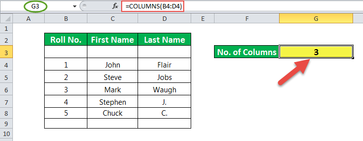
In the example of this column, cell G3 has a formula associated with it. So, G3 is a result cell.
The argument for the COLUMNS function in excel is a cell range, which is B4:D4. Here, B4 is a starting cell, and D4 is the ending cell.
The number of columns between these two cells is 3. So, the result is 3.
Example #2 – Total Cells In A Range

In this example, cell G4 has a formula associated with it. So, G4 is a result cell.
The formula is COLUMNS (B4: E8) * ROWS*B4: E8). Then, multiplication is performed between the total number of columns and a total number of rows for the given range of cells in the sheet.
Here, the total number of columns is four, and the total number of rows is 5. So, the total number of cells is 4*5 = 20.
Example #3 – Get The Address Of The First Cell In A Range

Here, the dataset is named data. Further, this data is used in the formula.
You may refer to the steps given below to name the dataset.
- Step 1: Select the cells.
- Step 2: Right-click and choose Define Name.
- Step 3: Name the dataset as data.

In the example of these columns, cell G6 has a formula associated with it. So, G6 is a result cell. The formula is to calculate the first cell in the dataset represented by the name data. The result is $B$4, i.e., B4, the last cell in the selected dataset.
The formula uses the ADDRESSES function, which has two parameters: row number and column number.
E.g., ADDRESS (8,5) returns $B$4. Here, 4 is the row number, and 2 is the column number. So, the function returns a cell denoted by these row and column numbers.
Here, a row number is calculated by
ROW(data)
And the column number is calculated by
COLUMN(data)
Example 4 – Get The Address Of The Last Cell In A Range

Here, the dataset is named data. Further, this data is used in the column’s formula in Excel. We can refer to the steps given below to name the dataset.
- Step 1: Select the cells.
- Step 2: Right-click and choose Define Name.
- Step 3: Name the dataset as data.

In this COLUMNS example, cell G5 has a formula associated with it. So, G5 is a result cell. The formula is to calculate the last cell in the dataset represented by the name data. The result is $E$8, i.e., E8, the last cell in the selected dataset.
The formula uses the ADDRESSES function, which has two parameters: row number and column number.
E.g., ADDRESS (8,5) returns $E$8. Here, 8 is the row number, and 5 is the column number. So, the function returns a cell denoted by these row and column numbers.
Here, the row number is calculated by
ROW(data)+ROWS(data-1)
And the column number is calculated by
COLUMN(data)+COLUMNS(data-1)
Important Things To Note
- The argument of the COLUMNS function in Excel can be a single cell address or a range of cells.
- The argument of the COLUMNS function cannot point to multiple references or cell addresses.
Frequently Asked Questions
1) What is the columns function in excel?
Columns Function in excel is a built-in excel function used to derive the number of columns used in the worksheet. The syntax of the COLUMNS function in excel is =COLUMNS(array). For example, consider the table with details of 3 employees.
We can calculate the number of columns used in the data using the columns function in excel.
Step 2: Select the range A1:C4 as shown in the below image.
Step 3: Press Enter key
We will get the result as shown in the below image.
2) When can we use the columns function in excel?
Columns Function in excel is used when we have to find the number of columns used in the data. Especially while working with large datasets, this function will be useful.
3) How to insert columns function in excel?
We can insert columns function in excel by selecting Formulas > Lookup & Reference in the Function Library group > COLUMNS function.
Alternatively, we can also type =COLUMNS and choose the cell array.
Columns Function in Excel Video
Recommended Articles
This article is a guide to Columns Function in Excel. We discuss the columns formula in Excel and how to use it, along with examples and downloadable templates. You can also go through our other suggested articles: –
- Excel Column Lock
- Excel Freeze Columns
- Group Column in Excel
- Column in Excel
- Break Links in Excel