
In an Excel worksheet, you may need to extract numbers from values in cells. And in this article, we will introduce you two methods to extract numbers from Excel cells.
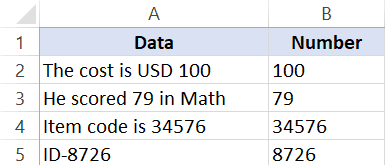
There are many cases that both numbers and texts are in same cells. In order to better analyze those values, you will need to extract the numbers and texts. The image below shows such an example. In column A, there are the ID and the name of products.
Now you need to input the product ID into column B in the worksheet. And below are the two methods that you can use.
Method 1: Excel Functions
In this part, we will show you how to use Excel functions to extract numbers from cells.
- Click the target cell where you need to input the numbers. In this example, we select cell B2.
- And then input the formula into the cell:
=LEFT(A2,3)
- After that, double click the fill handle of cell B2 and fill the same formula for the whole column. You will see that all the numbers will appear in column B.


You may find that in this example, all the numbers have the same digits. What if there are other forms of numbers in cells? Actually, there can be countless of number forms in cells. It is impossible to list all of them in just one article. And below we will have another example for you. In this image, the number digits are different for different products.
The function LEFT cannot take effect for all the different cells.
- Input another formula in cell B2:
=MID(A2,1,COUNT(1*MID(A2,ROW($1:$50),1)))
- And then press the shortcut keys “Ctrl +Shift +Enter” on the keyboard. By pressing these shortcut keys combo, this formula will turn into an array formula.
- Next double click the fill handle to fill the formula in the column.
In this formula, the 50 in the “ROW($1:$50)” is an estimated number. You can certainly change into other numbers according to the actual cell. This formula will first count how many numbers in the cell. And then the array formula will connect those numbers. Therefore, even if the number digits are different, you can still use this formula for this column.
When there are other forms of numbers in cells, you can also use functions. But the function may be very complex.
Method 2: VBA Macro
Except for using Excel functions, you can also use VBA to finish this task.
- Press the button “Alt + f11” on the keyboard.
- And then insert a new module.

- Now input the following codes into the new module:

Sub ExtractNumbersFromCells()
  Dim objRange As Range, nCellLength As Integer, nNumberPosition As Integer, strTargetNumber As String

  '  Initialization
  strTargetNumber = ""

  '  Go through all the cells in the target range
  For Each objRange In Range("A2:A4")
    nCellLength = Len(objRange)

    '  Extract numbers from cells
    For nNumberPosition = 1 To nCellLength
      If IsNumeric(Mid(objRange, nNumberPosition, 1)) Then
        strTargetNumber = strTargetNumber & Mid(objRange, nNumberPosition, 1)
      End If
    Next nNumberPosition

    objRange.Offset(0, 1) = strTargetNumber
    strTargetNumber = ""
  Next objRange
End Sub
You need to modify the range in the codes according to the actual worksheet.
- After that, run this macro. You can click the button “Run Sub” in the toolbar to run this macro. Besides, you can also press the button “F5” on the keyboard to run it.
- Next come back to the worksheet. You will find that all the product IDs are already in column B.


Even if there are other forms of numbers in cells, the numbers can be extracted by this macro. Therefore, this method is also very convenient.
A Comparison of the Two Methods
In the table below, we have found all the advantages and disadvantages of the two methods.
|
Comparison |
Excel Functions |
VBA Macro |
|
Advantages |
1. By using formulas, you can get the numbers in a column that even contains thousands of cells.
2. If you are not familiar with Excel VBA, this method can be your first choice. |
1. You can easily get the result by just one click in the editor.
2. Even if there are other forms of numbers, you can also extract them easily. |
|
Disadvantages |
1. The results are produced by formulas. You still need to copy and paste them as values.
2. When there are other forms of numbers in cells, you need to spend more time on getting a more complex formula. |
1. If you don’t know how to use VBA macro, you will easily meet with errors when running or modifying the codes.
2. |
The next time when you need to extract numbers from cells, you can use either of the two methods according to your need.
Get Your Data Storage in Order
When there are many Excel files in a storage device, you need to get them in order. Otherwise it is easily for you to meet with data disaster. When such accident happens, you can use an Excel recovery tool to repair corrupted xls data. Thus, your data and information will be safe. And the next time, remember to organize your Excel files.
Author Introduction:
Anna Ma is a data recovery expert in DataNumen, Inc., which is the world leader in data recovery technologies, including repair Word doc document error and outlook repair software products. For more information visit www.datanumen.com
Author: Oscar Cronquist Article last updated on December 16, 2021
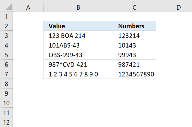
The following array formula, demonstrated in cell C3, extracts all numbers from a cell value:
=TEXTJOIN(, 1, TEXT(MID(B3, ROW($A$1:INDEX($A$1:$A$1000, LEN(B3))), 1), «#;-#;0;»))
To enter an array formula, type the formula in a cell then press and hold CTRL + SHIFT simultaneously, now press Enter once. Release all keys.
The formula bar now shows the formula with a beginning and ending curly bracket telling you that you entered the formula successfully. Don’t enter the curly brackets yourself.
If your cell contains more than a 1000 characters change this part of the formula $A$1:$A$1000 to perhaps $A$1:$A$2000 depending on how many characters you have.
Explaining array formula in cell C3
Step 1 — Count characters
The LEN function returns the number of characters in cell C3, so we can split each character into an array.
LEN(B3)
becomes
LEN(«123 BOA 214»)
returns 12.
Step 2 — Build cell reference
The INDEX function allows us to build a cell reference with as many rows as there are characters in cell B3.
$A$1:INDEX($A$1:$A$1000, LEN(B3))
becomes
$A$1:INDEX($A$1:$A$1000,12)
and returns $A$1:$A$12.
Step 3 — Create numbers based on row number of each cell in cell reference
The ROW function converts the cell reference to an array of numbers corresponding to the of each cell.
ROW($A$1:INDEX($A$1:$A$1000, LEN(B3)))
becomes
ROW($A$1:$A$12)
and returns {1; 2; 3; … 12}.
Step 4 — Create an array
The MID function splits each character in cell B3 into an array.
MID(B3, ROW($A$1:INDEX($A$1:$A$1000, LEN(B3))), 1)
becomes
MID(B3, {1; 2; 3; … 12}, 1)
and returns {«1″;»2″;»3″; … ;» «}
Step 5 — Filter out text letters
The TEXT function returns numerical values but leaves all other characters blank if you use the following pattern in the format_text argument: «#;-#;0;»
TEXT(value, format_text)
TEXT(MID(B3, ROW($A$1:INDEX($A$1:$A$1000, LEN(B3))), 1), «#;-#;0;»)
becomes
TEXT({«1″;»2″;»3″;» «;»B»;»O»;»A»;» «;»2″;»1″;»4″;» «}, «#;-#;0;»)
and returns
{«1»; «2»; «3»; «»; «»; «»; «»; «»; «2»; «1»; «4»; «»}.
Step 6 — Join numbers
The TEXTJOIN function introduced in Excel 2016 allows you to easily concatenate an array for values. In this case, it also ignores blank values in the array.
TEXTJOIN(, 1, TEXT(MID(B3, ROW($A$1:INDEX($A$1:$A$1000, LEN(B3))), 1), «#;-#;0;»))
becomes
TEXTJOIN(, 1, {«1»; «2»; «3»; «»; «»; «»; «»; «»; «2»; «1»; «4»; «»})
and returns 123214 in cell C3.
Get Excel *.xlsx file
How to extract numbers from a cell value.xlsx
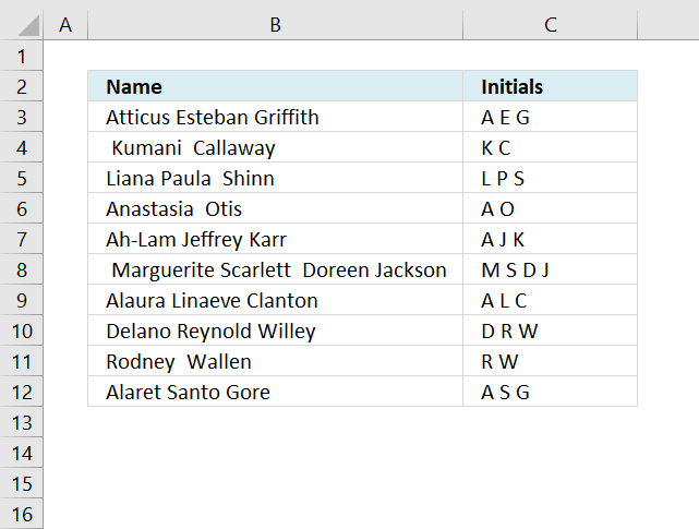
How to create name initials
The array formula in cell C3 extracts the first character from first, middle and last name. The formula works fine […]
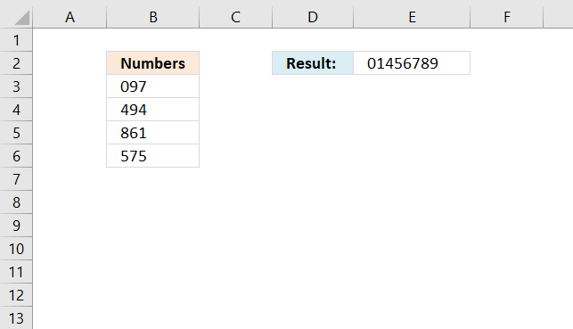
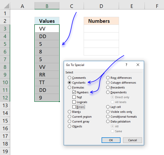
Extract numbers from a column
I this article I will show you how to get numerical values from a cell range manually and using an […]
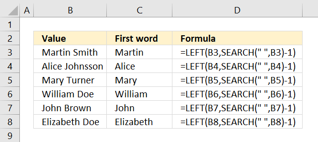
Extract first word in cell
The formula in cell C3 grabs the first word in B3 using a blank as the delimiting character. =LEFT(B3,SEARCH(» «,B3)-1) […]
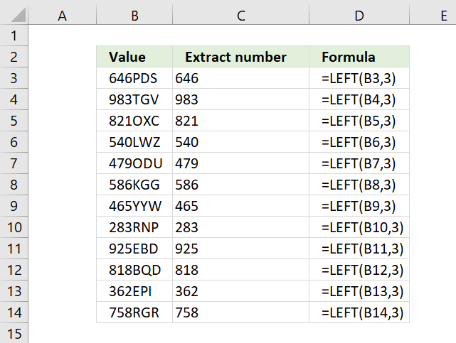
LEFT function for numbers
The LEFT function allows you to extract a string from a cell with a specific number of characters, however, if […]
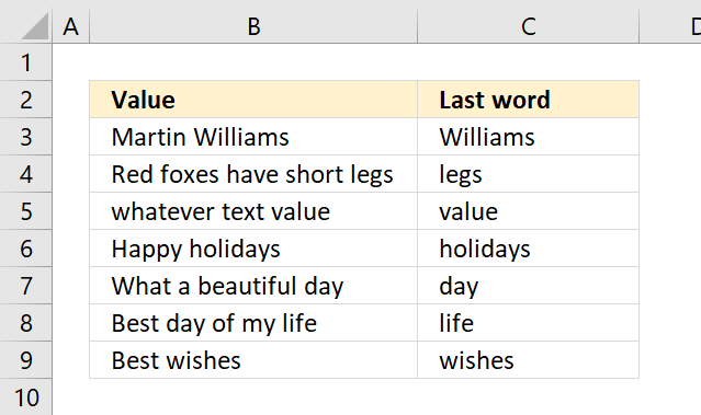
Extract last word in cell
Table of Contents Extract the last word Extract the last letter Extract the last number Get Excel *.xlsx file 1. […]
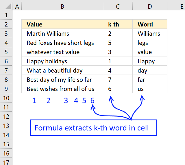
Extract n-th word in cell value
The formula displayed above in cell range D3:D9 extracts a word based on its position in a cell value. For […]
Latest updated articles.
More than 300 Excel functions with detailed information including syntax, arguments, return values, and examples for most of the functions used in Excel formulas.
More than 1300 formulas organized in subcategories.
Excel Tables simplifies your work with data, adding or removing data, filtering, totals, sorting, enhance readability using cell formatting, cell references, formulas, and more.
Allows you to filter data based on selected value , a given text, or other criteria. It also lets you filter existing data or move filtered values to a new location.
Lets you control what a user can type into a cell. It allows you to specifiy conditions and show a custom message if entered data is not valid.
Lets the user work more efficiently by showing a list that the user can select a value from. This lets you control what is shown in the list and is faster than typing into a cell.
Lets you name one or more cells, this makes it easier to find cells using the Name box, read and understand formulas containing names instead of cell references.
The Excel Solver is a free add-in that uses objective cells, constraints based on formulas on a worksheet to perform what-if analysis and other decision problems like permutations and combinations.
An Excel feature that lets you visualize data in a graph.
Format cells or cell values based a condition or criteria, there a multiple built-in Conditional Formatting tools you can use or use a custom-made conditional formatting formula.
Lets you quickly summarize vast amounts of data in a very user-friendly way. This powerful Excel feature lets you then analyze, organize and categorize important data efficiently.
VBA stands for Visual Basic for Applications and is a computer programming language developed by Microsoft, it allows you to automate time-consuming tasks and create custom functions.
A program or subroutine built in VBA that anyone can create. Use the macro-recorder to quickly create your own VBA macros.
UDF stands for User Defined Functions and is custom built functions anyone can create.
A list of all published articles.
Extracting numbers from a list of cells with mixed text is a common data cleaning task.
Unfortunately, there is no direct menu or function created in Excel to help us accomplish this.
In this tutorial we will look at three cases where you might have a list of mixed text, from which you might want to extract numbers:
- When the number is always at the end of the text
- When the number is always at the beginning of the text
- When the number can be anywhere in the text
We will look at three different formulas that can be used to extract the numbers in each case.
At the end of the tutorial, we will also take a look at some VBA code that you can use to accomplish the same.
Brace yourself, this might get a little complex!
Extracting a Number from Mixed Text when Number is Always at the End of the Text
Consider the following example:

Here, each cell has a mix of text and numbers, with the number always appearing at the end of the text. In such cases, we will need to use a combination of nested Excel functions to extract the numbers.
The functions we will use are:
- FIND – This function searches for a character or string in another string and returns its position.
- MIN – This function returns the smallest value in a list.
- LEFT – This function extracts a given number of characters from the left side of a string.
- SUBSTITUTE – This function replaces a particular substring of a given text with another substring.
- IFERROR – This function returns an alternative result or formula if it finds an error in a given formula.
Essentially, we will be using the above functions altogether to perform the following sequence of tasks:
- Find the position of the first numeric value in the given cell
- Extract and remove the text part of the given cell (by removing everything to the left of the first numeric digit)
The formula that we will use to extract the numbers from cell A2 is as follows:
=SUBSTITUTE(A2,LEFT(A2,MIN(IFERROR(FIND({0,1,2,3,4,5,6,7,8,9},A2),""))-1),"")
Let us break down this formula to understand it better. We will go from the inner functions to the outer functions:
- FIND({0,1,2,3,4,5,6,7,8,9},A2)
This function tries to find the positions of all the numbers (0-9) in the cell A2. Thus it returns an arrayformula:
{#VALUE!,#VALUE!,#VALUE!,#VALUE!,#VALUE!,#VALUE!,9,7,8,#VALUE!}
It returns a #VALUE! error for all digits except the 7th, 8th, and 9th digits because it was not able to find these numbers (0,1,2,3,4,5,9) in cell A2. It simply returns the positions of numbers 6,7 and 8 which are the 9th, 7th, and 8th characters respectively in A2.
- IFERROR(FIND({0,1,2,3,4,5,6,7,8,9},A2),””)
Next, the IFERROR function replaces all the error elements of the array with a blank (“”). As such it returns the arrayformula:
{“”,””,””,””,””,””,9,7,8,””}
- MIN(IFERROR(FIND({0,1,2,3,4,5,6,7,8,9},A2),””))
After this the MIN function finds the array element with least value. This is basically the position of the first numeric character in A2. The function now returns the value 7.
- LEFT(A2,MIN(IFERROR(FIND({0,1,2,3,4,5,6,7,8,9},A2),””))-1)
At this point we want to extract all text characters from A2 (so that we can remove them). So we want the LEFT function to extract all the characters starting backwards from the 7-1= 6th character. Thus we use the above formula. The result we get at this point is “arnold”. Notice we subtracted 1 from the second parameter of the LEFT function.
- SUBSTITUTE(A2,LEFT(A2,MIN(IFERROR(FIND({0,1,2,3,4,5,6,7,8,9},A2),””))-1),””)
Now all that’s left to do is remove the string obtained, by replacing it with a blank. This can be easily achieved by using the SUBSTITUTE function: We finally get the numeric characters in the mixed text, which is “786”.
Once you are done entering the formula, make sure you press CTRL+SHIFT+Enter, instead of just the return key. This is because the formula involves arrays.
In a nutshell, here’s what’s happening when you break down the formula:
=SUBSTITUTE(A2,LEFT(A2,MIN(IFERROR(FIND({0,1,2,3,4,5,6,7,8,9},A2),””))-1),””)
=SUBSTITUTE(A2,LEFT(A2,MIN(IFERROR({{#VALUE!,#VALUE!,#VALUE!,#VALUE!,#VALUE!,#VALUE!,9,7,8,#VALUE!}),””))-1),””)
=SUBSTITUTE(A2,LEFT(A2,MIN({“”,””,””,””,””,””,9,7,8,””}))-1),””)
=SUBSTITUTE(A2,”arnold”,””)
=786
When you drag the formula down to the rest of the cells, here’s the result you get:

Also read: How to Generate Random Letters in Excel?
Extracting a Number from Mixed Text when Number is Always at the Beginning of the Text
Now let us consider the case where the numbers are always at the beginning of the Text.
Consider the following example:

Here, each cell has a mix of text and numbers, with the number always appearing at the beginning of the text. In such cases, we will again need to use a combination of nested Excel functions to extract the numbers.
In addition to the functions we used in the previous formula, we are going to use two additional functions. These are:
- MAX – This function returns the largest value in a list
- RIGHT – This function extracts a given number of characters from the right side of a string
- LEN – This function finds the length of (number of characters in) a given string.
Essentially, we will be using these functions altogether to perform the following sequence of tasks:
- Find the position of the last numeric value in the given cell
- Extract and remove the text part of the given cell (by removing everything to the right of the last numeric digit)
The formula that we will use to extract the numbers from cell A2 is as follows:
=SUBSTITUTE(A2,RIGHT(A2,LEN(A2)-MAX(IFERROR(FIND({0,1,2,3,4,5,6,7,8,9},A2),""))),"")
Let us break down this formula to understand it better. We will go from the inner functions to the outer functions:
- FIND({0,1,2,3,4,5,6,7,8,9},A2)
This function tries to find the positions of all the numbers (0-9) in the cell A2. Thus it returns an arrayformula:
{#VALUE!,#VALUE!,1,#VALUE!,#VALUE!,2,#VALUE!,#VALUE!,#VALUE!,#VALUE!}
It returns a #VALUE! error for all digits except the 3rd and 6th digits because it was not able to find these numbers (0,1,3,4,6,7,8,9) in cell A2. It simply returns the positions of numbers 2 and 5 which are the 1st and 2nd characters respectively in A2.
- IFERROR(FIND({0,1,2,3,4,5,6,7,8,9},A2),””)
Next, the IFERROR function replaces all the error elements of the array with a blank. As such it returns the array formula:
{“”,””,1,””,””,2,””,””,””,””}
- MAX(IFERROR(FIND({0,1,2,3,4,5,6,7,8,9},A2),””))
After this the MAX function finds the array element with the highest value. This is basically the position of the last numeric character in A2. The function now returns the value 2.
- LEN(A2)-MAX(IFERROR(FIND({0,1,2,3,4,5,6,7,8,9},A2),””))
At this point we want to extract all text characters from A2 (so that we can remove them). We need to specify how many characters we want to remove. This is obtained by computing the length of the string in A2 minus the position of the last numeric value.Thus we will get the value 8-2 = “6”.
- RIGHT(A2,LEN(A2)-MAX(IFERROR(FIND({0,1,2,3,4,5,6,7,8,9},A2),””)))
We can now use the RIGHT function to extract 6 characters starting from the 2nd character onwards. The result we get at this point is “arnold”.
- SUBSTITUTE(A2,RIGHT(A2,LEN(A2)-MAX(IFERROR(FIND({0,1,2,3,4,5,6,7,8,9},A2),””))),””)
Now all that’s left to do is remove this string by replacing it with a blank. This is easily achieved by using the SUBSTITUTE function. We finally get the numeric characters in the mixed text, which is “25”.
Again, once you are done entering the formula, don’t forget to press CTRL+SHIFT+Enter, instead of just the return key.
In a nutshell, here’s what’s happening when you break down the formula:
=SUBSTITUTE(A7,RIGHT(A7,LEN(A7)-MAX(IFERROR(FIND({0,1,2,3,4,5,6,7,8,9},A7),””))),””)
=SUBSTITUTE(A7,RIGHT(A7,LEN(A7)-MAX(IFERROR({#VALUE!,#VALUE!,1,#VALUE!,#VALUE!,2,#VALUE!,#VALUE!,#VALUE!,#VALUE!}
),””))),””)
=SUBSTITUTE(A7,RIGHT(A7,LEN(A7)-MAX({“”,””,1,””,””,2,””,””,””,””}
)),””)
=SUBSTITUTE(A7,RIGHT(A7,LEN(A7)-2),””)
=SUBSTITUTE(A7,RIGHT(A7,8-2),””)
=SUBSTITUTE(A7,”arnold”,””)
=25
When you drag the formula down to the rest of the cells, here’s the result you get:

Extracting a Number from Mixed Text when Number can be Anywhere in the Text
Finally let us consider the case where the numbers can be anywhere in the text, be it the beginning, end or middle part of the text.
Let’s take a look at the following example:

Here, each cell has a mix of text and numbers, where the number appears in any part of the text. In such cases, we will need to use a combination of nested Excel functions to extract the numbers.
Here are the functions that we are going to use this time:
- INDIRECT – This function simply returns a reference to a range of values.
- ROW – This function returns a row number of a reference.
- MID – This function extracts a given number of characters from the middle of a string.
- TEXTJOIN – This function combines text from multiple ranges or strings using a specified delimiter between them.
Note that the formula discussed in this section will work only in Excel version 2016 onwards as it uses the newly introduced TEXTJOIN function. If you are using an older version of Excel, then you may consider using the VBA method instead (discussed in the next section).
In this method, we will essentially be using the above functions altogether to perform the following sequence of tasks:
- Break up the given text into an array of individual characters
- Find out and remove all characters that are not numbers
- Combine the remaining characters into a full number
The formula that we will use to extract the numbers from cell A2 is as follows:
=TEXTJOIN("",TRUE,IFERROR(MID(A2,ROW(INDIRECT("1:"&LEN(A2))),1)*1,""))
Let us break down this formula to understand it better. We will go from the inner functions to the outer functions:
- LEN(A2)
This function finds the length of the string in cell A2. In our case it returns 13.
- INDIRECT(“1:”&LEN(A2))
This function just returns a reference to all the rows from row 1 to row 12.
- ROW(INDIRECT(“1:”&LEN(A2)))
Now this function returns the row numbers of each of these rows. In other words, it simply returns an array of numbers 1 to 12. This function thus returns the array:
{1;2;3;4;5;6;7;8;9;10;11;12;13}
Note: We use the ROW() function instead of simply hard-coding an array of numbers 1 to 12 because we want to be able to customize this formula depending on the size of the string being worked on. This will ensure that the function adjusts itself when copied to another cell. ·
- MID(A2,ROW(INDIRECT(“1:”&LEN(A2))),1)
Next the MID function extracts the character from A2 that corresponds to each position specified in the array. In other words, it returns an array containing each character of the text in A2 as a separate element, as follows:
{“a”;”r”;”n”;”o”;”l”;”d”;”1″;”4″;”3″;”b”;”l”;”u”;”e”}
- IFERROR(MID(A2,ROW(INDIRECT(“1:”&LEN(A2))),1)*1,””)
After this, the IFERROR function replaces all the elements of the array that are non-numeric. This is because it checks if the array element can be multiplied by 1. If the element is a number, it can easily be multiplied to return the same number. But if the element is a non-numeric character, then it cannot be multiplied with 1 and thus returns an error.
The IFERROR function here specifies that if an element gives an error on multiplication, the result returned will be blank. As such it returns the arrayformula:
{“”;””;””;””;””;””;1;4;3;””;””;””;””}
- TEXTJOIN(“”,TRUE,IFERROR(MID(A2,ROW(INDIRECT(“1:”&LEN(A2))),1)*1,””))
Finally, we can simply combine the array elements together using the TEXTJOIN function. The TEXTJOIN function here combines the string characters that remain (which are the numbers only) and ignores the empty string characters. We finally get the numeric characters in the mixed text, which is “143”.
Once you are done entering the formula, don’t forget to press CTRL+SHIFT+Enter, instead of just the return key.
In a nutshell, here’s what’s happening when you break down the formula:
=TEXTJOIN(“”,TRUE,IFERROR(MID(A2,ROW(INDIRECT(“1:”&LEN(A2))),1)*1,””))
=TEXTJOIN(“”,TRUE,IFERROR(MID(A2,ROW(INDIRECT(“1:”&13)),1)*1,””))
=TEXTJOIN(“”,TRUE,IFERROR(MID(A2,{1;2;3;4;5;6;7;8;9;10;11;12;13},1)*1,””))
=TEXTJOIN(“”,TRUE,IFERROR({“a”;”r”;”n”;”o”;”l”;”d”;”1″;”4″;”3″;”b”;”l”;”u”;”e”}
*1,””))
=TEXTJOIN(“”,TRUE,IFERROR(MID(A2,{1;2;3;4;5;6;7;8;9;10;11;12;13},1)*1,””))
=TEXTJOIN(“”,TRUE, {“”;””;””;””;””;””;1;4;3;””;””;””;””})
=143
When you drag the formula down to the rest of the cells, here’s the result you get:

Using VBA to Extract Number from Mixed Text in Excel
The above method works well enough in extracting numbers from anywhere in a mixed text.
However, it requires one to use the TEXTJOIN function, which is not available in older Excel versions (versions before Excel 2016).
If you’re on a version of Excel that does not support TEXTJOIN, then you can, instead, use a snippet of VBA code to get the job done.
If you have never used VBA before, don’t worry. All you need to do is copy the code below into your VBA developer window and run it on your worksheet data.
Here’s the code that you will need to copy:
'Code by Steve Scott from spreadsheetplanet.com
Function ExtractNumbers(CellRef As String)
Dim StringLength As Integer
StringLength = Len(CellRef)
For i = 1 To StringLength
   If (IsNumeric(Mid(CellRef, i, 1))) Then Result = Result & Mid(CellRef, i, 1)
Next i
ExtractNumbers = Result
End Function
The above code creates a user-defined function called ExtractNumbers() that you can use in your worksheet to extract numbers from mixed text in any cell.
To get to your VBA developer window, follow these steps:
- From the Developer tab, select Visual Basic.

- Once your VBA window opens, Click Insert->Module. That’s it, you can now start coding.

Type or copy-paste the above lines of code into the module window. Your code is now ready to run.

Now, whenever you want to extract numbers from a cell, simply type the name of the function, passing the cell reference as a parameter. So to extract numbers from a cell A2, you will simply need to type the function as follows in a cell:
=ExtractNumbers(A2)

Explanation of the Code
Now let us take some time to understand how this code works.
- In this code, we defined a function named ExtractNumbers, that takes the string in the cell we want to work on. We assigned the name CellRef to this string.
Function ExtractNumbers(CellRef As String)
- We created a variable named StringLength, that will hold the length of the string, CellRef.
Dim StringLength As Integer
StringLength = Len(CellRef)
- Next, we loop through each character in the string CellRef and find out if it is a number. We use the function Mid(CellRef, i, 1) to extract a character from the string at each iteration of the loop. We also use the IsNumeric() function to find out if the extracted character is a number. Each extracted numeric character is combined together into a string called Result.
For i = 1 To StringLength
If (IsNumeric(Mid(CellRef, i, 1))) Then Result = Result & Mid(CellRef, i, 1)
Next i
- This Result is then returned by the function.
ExtractNumbers = Result
Note that since the workbook now has VBA code in it, you need to save it with .xls or .xlsm extension.
You can also choose to save this to your Personal Macro Workbook, if you think you will be needing to run this code a lot. This will allow you to run the code on any Excel workbook of yours.
Well, that was a lot!
In this tutorial, we showed you how to extract numbers from mixed text in excel.
We saw three cases where the numbers are situated in different parts of the text. We also showed you how to use VBA to get the task done quickly.
Other Excel articles you may also like:
- How to Extract URL from Hyperlinks in Excel (Using VBA Formula)
- How to Reverse a Text String in Excel (Using Formula & VBA)
- How to Add Text to the Beginning or End of all Cells in Excel
- How to Remove Text after a Specific Character in Excel (3 Easy Methods)
- How to Separate Address in Excel?
- How to Extract Text After Space Character in Excel?
- How to Find the Last Space in Text String in Excel?
- How to Remove Space before Text in Excel
Microsoft Excel is great at working with both numbers and text—but if you’re using both in the same cell, you might run into some difficulty. Fortunately, you can extract numbers or text from cells to work with your data more efficiently. We demonstrate several options, depending on the format that your data is currently in.
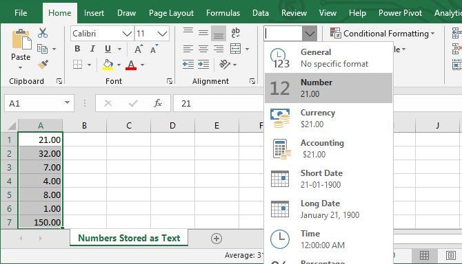
Excel Numbers Formatted as Text
This is a common situation, and—fortunately—very easy to deal with. Sometimes, cells that contain only numbers are incorrectly labeled or formatted as text, preventing Microsoft Excel from using them in operations.
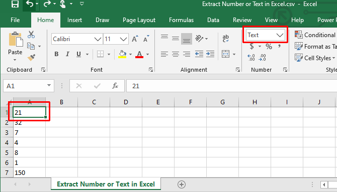
You can see in the image below that the cells in column A are formatted as text, as indicated by the number format box. You might also see a green flag in the top left corner of each cell.
Convert Text to Number in Excel
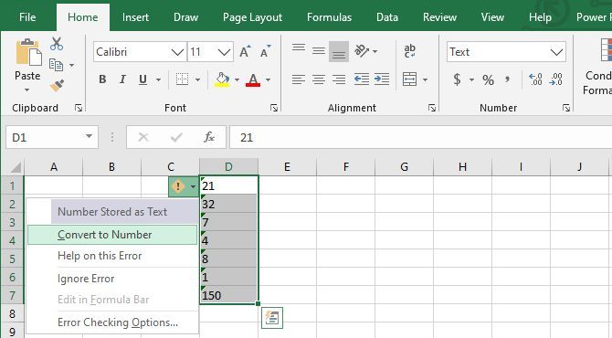
If you see the green flag in the top left corner, select one or more cells, click the warning sign, and select Convert to Number.
Otherwise, select the cells and, in the Number Format menu in the Ribbon, select the default Number option.
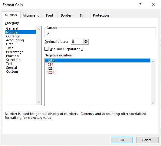
If you need more granular options, right-click the highlighted cell/s and select Format Cells, which will open the respective menu. Here, you can customize the number format and add or remove decimals, add a 1,000 separator, or manage negative numbers.
Obviously, you can also use the Ribbon or Format Cells options outlined above to convert a number to text, or text to currency, time, or any other format you desire.
Apply Number Formatting With Excel’s Paste Special
For this method to work, you’ll need to enter a number (any number) into a cell; it’s important that this cell is also formatted as a number. Copy that cell. Now, select all the cells that you want to convert to the number format, go to Home > Paste > Paste Special, select Formats to paste only the formatting of the cell you copied initially, then click OK.
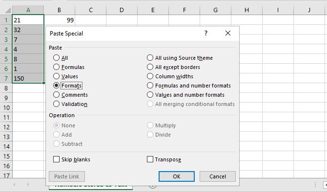
This operation applies the format of the cell you copied to all selected cells, even text cells.
Now we get to the hard part: getting numbers out of cells that contain multiple formats of input. If you have a number and a unit (like «7 shovels,» as we have below), you’ll run into this problem. To solve it, we’re going to look at a couple different ways to split cells into numbers and text, letting you work with each individually.
Separate Numbers From Text
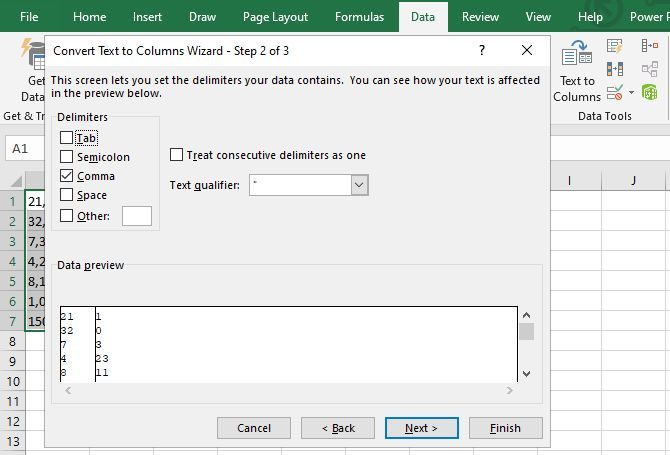
If you have a lot of cells that contain a mix of numbers and text or multiples of both, separating them manually might take a monumental amount of time. To get through the process faster, you can use Microsoft Excel’s Text to Columns function.
Select the cells that you want to convert, go to Data > Text to Columns, and use the wizard to make sure the cells come out correctly. For the most part, you’ll just need to click Next and Finish, but do make sure you pick a matching delimiter; in this example, a comma.
If you only have one- and two-digit numbers, the Fixed Width option can be useful too, as it will only split off the first two or three characters of the cell. You can even create a number of splits that way.
Note: Cells formatted as text will not automatically emerge with a number formatting (or vice versa), meaning you might still have to convert these cells as described above.
This method is a bit cumbersome, but works very well on small datasets. What we assume here is that a space separates the number and text, though the method also works for any other delimiter.
The main function we’ll be using here is LEFT, which returns the leftmost characters from a cell. As you can see in our dataset above, we have cells with one-, two-, and three-character numbers, so we’ll need to return the leftmost one, two, or three characters from the cells. By combining LEFT with the SEARCH function, we can return everything to the left of the space. Here’s the function:
=LEFT(A1, SEARCH(" ", A1, 1))
This will return everything to the left of the space. Using the fill handle to apply the formula to the rest of the cells, this is what we get (you can see the formula in the function bar at the top of the image):
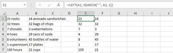
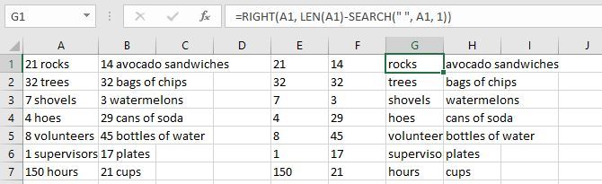
As you can see, we now have all the numbers isolated, so we can manipulate them. Want to isolate the text as well? We can use the RIGHT function in the same way:
=RIGHT(A1, LEN(A1)-SEARCH(" ", A1, 1))
This returns X characters from the right side of the cell, where x is the total length of the cell minus the number of characters to the left of the space.
Now you can also manipulate the text. Want to combine them again? Just use the CONCATENATE function with all the cells as inputs:
=CONCATENATE(E1, F1)
Obviously, this method works best if you just have numbers and units, and nothing else. If you have other cell formats, you might have to get creative with formulas to get everything to work right. If you have a giant dataset, it’ll be worth the time it takes to get the formula figured out!
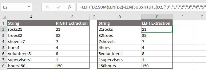
Now what if there’s no delimiter separating your number and text?
If you’re extracting the number from the left or right of the string, you can use a variation of the LEFT or RIGHT formula discussed above:
=LEFT(A1,SUM(LEN(A1)-LEN(SUBSTITUTE(A1,{"0","1","2","3","4","5","6","7","8","9"},""))))
=RIGHT(A1,SUM(LEN(A1)-LEN(SUBSTITUTE(A1,{"0","1","2","3","4","5","6","7","8","9"},""))))
This will return all numbers from the left or right of the string.
If you’re extracting the number from the right of the string, you can also use a two-step process. First, determine the location of your first digit in the string using the MIN function. Then, you can feed that information into a variation of the RIGHT formula, to split your numbers from your texts.
=MIN(SEARCH({0,1,2,3,4,5,6,7,8,9},A1&"0123456789"))
=RIGHT(A1, LEN(A1)-B1+1)
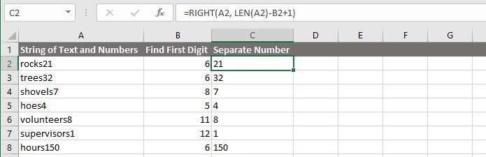
Note: When you use these formulas, remember that you might have to adjust the column characters and cell numbers.
With the strategies above, you should be able to extract numbers or text out of most mixed-format cells that are giving you trouble. Even if they don’t, you can probably combine them with some powerful text functions included in Microsoft Excel to get the characters you’re looking for. However, there are some much more complicated situations that call for more complicated solutions.
For example, I found a forum post where someone wanted to extract the numbers from a string like «45t*&65/», so that he would end up with «4565.» Another poster gave the following formula as one way to do it:
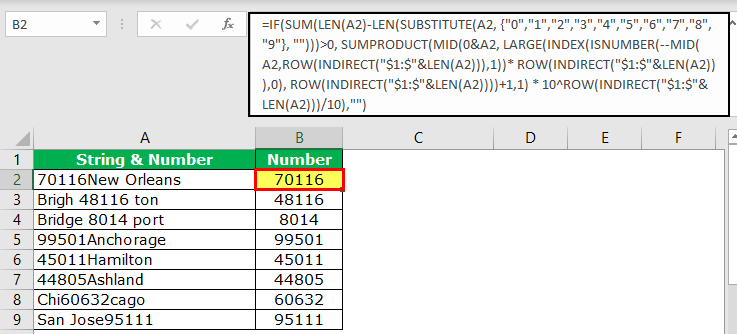
=SUMPRODUCT(MID(0&A1,LARGE(INDEX(ISNUMBER(--MID(A1,ROW($1:$25),1))*ROW($1:$25),0),ROW($1:$25))+1,1)*10^ROW($1:$25)/10)
To be completely honest, I have no idea how it works. But according to the forum post, it will take the numbers out of a complicated string of numbers and other characters. The point is that, with enough time, patience, and effort, you can extract numbers and text from just about anything! You just have to find the right resources.
After some more Excel tips? Here’s how to copy formulas in Excel.
I’ve got a column where cells contain phone numbers in the following format:
To: +6112312414 Will Smith To: +61832892357 Tom Hopkins To: +447857747717 Julius Caesar
Or
From: +44712423110 Jack Russel To: 112312414 Mr XYZ To: +61832892357 Hulk
I need to extract the recipient phone numbers in a separate column, names not required e.g.
+6112312414, +61832892357, +447857747717 for the first example and 112312414, +61832892357 for the second example. Can someone please help with this? Thanks!
asked Sep 26, 2018 at 17:47
![]()
5
Try the following User Defined Function:
Public Function PhoneList(st As String) As String
    Dim v As String
    PhoneList = ""
    v = Replace(st, "To: ", Chr(1))
    arr = Split(v, " ")
    For Each a In arr
        If InStr(a, Chr(1)) > 0 Then
            PhoneList = PhoneList & ", " & a
        End If
    Next a
    PhoneList = Replace(PhoneList, Chr(1), "")
    PhoneList = Mid(PhoneList, 3, 9999)
End Function

answered Sep 26, 2018 at 18:12
![]()
Gary’s StudentGary’s Student
95.3k9 gold badges58 silver badges98 bronze badges
4
You could extract the data from the column using text to column. Apply the other method and select the colon as extraction :. Then you would be left with the a ‘space’+number…note the ‘space’ denotes just one white space.
Next, use the replace all column to remove the space, and you are left with just the +number.
answered Sep 26, 2018 at 17:53
![]()
3
Select a blank cell that is adjacent to the list you want to extract number only, and type this formula =SUMPRODUCT(MID(0&A2,LARGE(INDEX(ISNUMBER(--MID(A2,ROW($1:$25),1))* ROW($1:$25),0),ROW($1:$25))+1,1)*10^ROW($1:$25)/10)
(A2 stands the first data you want to extract numbers only from the list), then press Shift + Ctrl + Enter buttons, and drag the fill handle to fill the range you need to apply this formula.
answered Sep 26, 2018 at 18:01
![]()
IrfanuddinIrfanuddin
2,1951 gold badge15 silver badges28 bronze badges
0
Use TEXTJOIN as an array
=TEXTJOIN(", ",TRUE,IF(TRIM(MID(SUBSTITUTE(A1," ",REPT(" ",99)),(ROW($A$1:INDEX(A:A,LEN(A1)-LEN(SUBSTITUTE(A1," ",""))+1))-1)*99+1,99))="To:",TRIM(MID(SUBSTITUTE(A1," ",REPT(" ",99)),(ROW($A$1:INDEX(A:A,LEN(A1)-LEN(SUBSTITUTE(A1," ",""))+1)))*99+1,99)),""))
Being an array formula it must be confirmed with Ctrl-Shift-Enter instead of Enter when exiting edit mode.
TEXTJOIN was introduced with Office 365 Excel

answered Sep 26, 2018 at 18:25
![]()
Scott CranerScott Craner
146k9 gold badges47 silver badges80 bronze badges
1
First you should convert the cell to columns, after that you should go to a blank cell and write this command =B1 & » » & «,» & » » & F1 & » » & «,» & » » & J1
this command is for your first example because the reference cells in the command contain the numbers
if you want to apply the same command just modify the reference cell as you want

answered Sep 26, 2018 at 19:01
![]()
This article will explain you how to extract the numbers from a cell containing numbers and letters.
To do that, we will use the new functions of Excel 365 ; FILTER and SEQUENCE
Understand the logic applied
To be able to extract the numbers and letters from the same cell, we have no choice ; extract each single character into the cell.
- This task is now possible with the new SEQUENCE function and the MID function .
- Next, we will perform a test to find out if each one of these characters is a number or not.
- Finally, when the test is true. So we just keep the numbers.
Step 1: Extract each character from the cell
The SEQUENCE function generates a series of number between 2 values. For instance to create a series of number between 1 and 5 in column, you will write
=SEQUENCE(,5)

The trick here, is to use the SEQUENCE function to split each character of the cells with this formula with the MID function. Also, the LEN function will return the exact number of characters in each cells.
=MID(A2,SEQUENCE(,LEN(A2)),1)

Step 2: Test if each character is a number or not
Then we need to perform a test on each one of these characters to find out if it’s a number or not.
So of course here, using the ISNUMBERfunction seems logical. However, at this stage, each of the cells contains text 😕🤨
=ISNUMBER(MID(A2,SEQUENCE(,LEN(A2)),1))

We can easily correct this with the function VALUE. VALUE will automatically convert a character to a number if needed.
=ISNUMBER(VALUE(MID(A2,SEQUENCE(LEN(A2)),1)))

To highlight the cells when the result is true, I have used the following conditional formatting rule
=B2=TRUE
Step 3: Isolate the numbers
Now, to group only the numbers (when the test is TRUE), we use the FILTER function.
The first argument of the FILTER function is the first formula we have build on step 1
The second argument is the test build on the step 2
=FILTER(MID(A2,SEQUENCE(,LEN(A2)),1),ISNUMBER(VALUE(MID(A2,SEQUENCE(,LEN(A2)),1))))

Step 4: Group the numbers together
This is the last step 😀 We just have to group the previous result with the TEXTJOIN function.
=TEXTJOIN(«»,,FILTER(VALUE(MID(A2,SEQUENCE(LEN(A2)),1)),ISNUMBER(VALUE(MID(A2,SEQUENCE(LEN(A2)),1)))))

Other solution
Rick Rothsein, another Microsoft Excel MVP, has another approach to solve this problem.
The formula he proposes is this one
=CONCAT(IFERROR(0+MID(A1,SEQUENCE(LEN(A1)),1),»»))
He reused the technique to combine MID, SEQUENCE and LEN but instead of using the FILTER function, he just do a calculation with 0. So, when it’s letter + 0, it’s an error. When it’s 0 + number, the formula returns a number. This is why he used IFERROR to keep only the numbers (clever 😉)
Thanks a lot Rick for sharing your formula 👏👏👏
ТРЕНИНГИ
Быстрый старт
Расширенный Excel
Мастер Формул
Прогнозирование
Визуализация
Макросы на VBA
КНИГИ
Готовые решения
Мастер Формул
Скульптор данных
ВИДЕОУРОКИ
Бизнес-анализ
Выпадающие списки
Даты и время
Диаграммы
Диапазоны
Дубликаты
Защита данных
Интернет, email
Книги, листы
Макросы
Сводные таблицы
Текст
Форматирование
Функции
Всякое
Коротко
Подробно
Версии
Вопрос-Ответ
Скачать
Купить
ПРОЕКТЫ
ОНЛАЙН-КУРСЫ
ФОРУМ
Excel
Работа
PLEX
© Николай Павлов, Planetaexcel, 2006-2022
info@planetaexcel.ru
Использование любых материалов сайта допускается строго с указанием прямой ссылки на источник, упоминанием названия сайта, имени автора и неизменности исходного текста и иллюстраций.
Техническая поддержка сайта
|
ООО «Планета Эксел» ИНН 7735603520 ОГРН 1147746834949 |
ИП Павлов Николай Владимирович ИНН 633015842586 ОГРНИП 310633031600071 |
Watch Video – How to Extract Numbers from text String in Excel (Using Formula and VBA)
There is no inbuilt function in Excel to extract the numbers from a string in a cell (or vice versa – remove the numeric part and extract the text part from an alphanumeric string).
However, this can be done using a cocktail of Excel functions or some simple VBA code.
Let me first show you what I am talking about.
Suppose you have a data set as shown below and you want to extract the numbers from the string (as shown below):
The method you choose will also depend on the version of Excel you’re using:
- For versions prior to Excel 2016, you need to use slightly longer formulas
- For Excel 2016, you can use the newly introduced TEXTJOIN function
- VBA method can be used in all the versions of Excel
Click here to download the example file
Extract Numbers from String in Excel (Formula for Excel 2016)
This formula will work only in Excel 2016 as it uses the newly introduced TEXTJOIN function.
Also, this formula can extract the numbers that are at the beginning, end or middle of the text string.
Note that the TEXTJOIN formula covered in this section would give you all the numeric characters together. For example, if the text is “The price of 10 tickets is USD 200”, it will give you 10200 as the result.
Suppose you have the dataset as shown below and you want to extract the numbers from the strings in each cell:
Below is the formula that will give you numeric part from a string in Excel.
=TEXTJOIN("",TRUE,IFERROR((MID(A2,ROW(INDIRECT("1:"&LEN(A2))),1)*1),""))
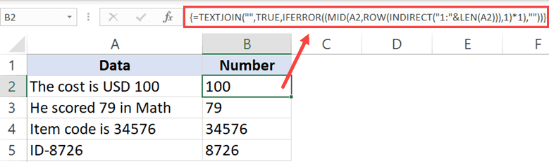
This is an array formula, so you need to use ‘Control + Shift + Enter‘ instead of using Enter.
In case there are no numbers in the text string, this formula would return a blank (empty string).
How does this formula work?
Let me break this formula and try and explain how it works:
- ROW(INDIRECT(“1:”&LEN(A2))) – this part of the formula would give a series of numbers starting from one. The LEN function in the formula returns the total number of characters in the string. In the case of “The cost is USD 100”, it will return 19. The formulas would thus become ROW(INDIRECT(“1:19”). The ROW function will then return a series of numbers – {1;2;3;4;5;6;7;8;9;10;11;12;13;14;15;16;17;18;19}
- (MID(A2,ROW(INDIRECT(“1:”&LEN(A2))),1)*1) – This part of the formula would return an array of #VALUE! errors or numbers based on the string. All the text characters in the string become #VALUE! errors and all numerical values stay as-is. This happens as we have multiplied the MID function with 1.
- IFERROR((MID(A2,ROW(INDIRECT(“1:”&LEN(A2))),1)*1),””) – When IFERROR function is used, it would remove all the #VALUE! errors and only the numbers would remain. The output of this part would look like this – {“”;””;””;””;””;””;””;””;””;””;””;””;””;””;””;””;1;0;0}
- =TEXTJOIN(“”,TRUE,IFERROR((MID(A2,ROW(INDIRECT(“1:”&LEN(A2))),1)*1),””)) – The TEXTJOIN function now simply combines the string characters that remains (which are the numbers only) and ignores the empty string.
Pro Tip: If you want to check the output of a part of the formula, select the cell, press F2 to get into the edit mode, select the part of the formula for which you want the output and press F9. You will instantly see the result. And then remember to either press Control + Z or hit the Escape key. DO NOT hit the enter key.
Download the Example File

You can also use the same logic to extract the text part from an alphanumeric string. Below is the formula that would get the text part from the string:
=TEXTJOIN("",TRUE,IF(ISERROR(MID(A2,ROW(INDIRECT("1:"&LEN(A2))),1)*1),MID(A2,ROW(INDIRECT("1:"&LEN(A2))),1),""))
A minor change in this formula is that IF function is used to check if the array we get from MID function are errors or not. If it’s an error, it keeps the value else it replaces it with a blank.
Then TEXTJOIN is used to combine all the text characters.
Caution: While this formula works great, it uses a volatile function (the INDIRECT function). This means that in case you use this with a huge dataset, it may take some time to give you the results. It’s best to create a backup before you use this formula in Excel.
Extract Numbers from String in Excel (for Excel 2013/2010/2007)
If you have Excel 2013. 2010. or 2007, you can not use the TEXTJOIN formula, so you will have to use a complicated formula to get this done.
Suppose you have a dataset as shown below and you want to extract all the numbers in the string in each cell.
The below formula will get this done:
=IF(SUM(LEN(A2)-LEN(SUBSTITUTE(A2, {"0","1","2","3","4","5","6","7","8","9"}, "")))>0, SUMPRODUCT(MID(0&A2, LARGE(INDEX(ISNUMBER(--MID(A2,ROW(INDIRECT("$1:$"&LEN(A2))),1))* ROW(INDIRECT("$1:$"&LEN(A2))),0), ROW(INDIRECT("$1:$"&LEN(A2))))+1,1) * 10^ROW(INDIRECT("$1:$"&LEN(A2)))/10),"")
In case there is no number in the text string, this formula would return blank (empty string).
Although this is an array formula, you don’t need to use ‘Control-Shift-Enter’ to use this. A simple enter works for this formula.
Credit to this formula goes to the amazing Mr. Excel forum.
Again, this formula will extract all the numbers in the string no matter the position. For example, if the text is “The price of 10 tickets is USD 200”, it will give you 10200 as the result.
Caution: While this formula works great, it uses a volatile function (the INDIRECT function). This means that in case you use this with a huge dataset, it may take some time to give you the results. It’s best to create a backup before you use this formula in Excel.
Separate Text and Numbers in Excel Using VBA
If separating text and numbers (or extracting numbers from the text) is something you have to often, you can also use the VBA method.
All you need to do is use a simple VBA code to create a custom User Defined Function (UDF) in Excel, and then instead of using long and complicated formulas, use that VBA formula.
Let me show you how to create two formulas in VBA – one to extract numbers and one to extract text from a string.
Extract Numbers from String in Excel (using VBA)
In this part, I will show you how to create the custom function to get only the numeric part from a string.
Below is the VBA code we will use to create this custom function:
Function GetNumeric(CellRef As String)
Dim StringLength As Integer
StringLength = Len(CellRef)
For i = 1 To StringLength
If IsNumeric(Mid(CellRef, i, 1)) Then Result = Result & Mid(CellRef, i, 1)
Next i
GetNumeric = Result
End Function
Here are the steps to create this function and then use it in the worksheet:
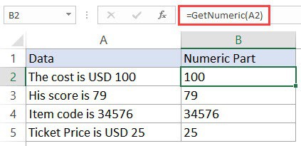
Now, you will be able to use the GetText function in the worksheet. Since we have done all the heavy lifting in the code itself, all you need to do is use the formula =GetNumeric(A2).
This will instantly give you only the numeric part of the string.
Note that since the workbook now has VBA code in it, you need to save it with .xls or .xlsm extension.
Download the Example File
In case you have to use this formula often, you can also save this to your Personal Macro Workbook. This will allow you to use this custom formula in any of the Excel workbooks that you work with.
Extract Text from a String in Excel (using VBA)
In this part, I will show you how to create the custom function to get only the text part from a string.
Below is the VBA code we will use to create this custom function:
Function GetText(CellRef As String)
Dim StringLength As Integer
StringLength = Len(CellRef)
For i = 1 To StringLength
If Not (IsNumeric(Mid(CellRef, i, 1))) Then Result = Result & Mid(CellRef, i, 1)
Next i
GetText = Result
End Function
Here are the steps to create this function and then use it in the worksheet:
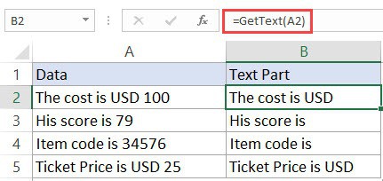
Now, you will be able to use the GetNumeric function in the worksheet. Since we have done all the heavy lifting in the code itself, all you need to do is use the formula =GetText(A2).
This will instantly give you only the numeric part of the string.
Note that since the workbook now has VBA code in it, you need to save it with .xls or .xlsm extension.
In case you have to use this formula often, you can also save this to your Personal Macro Workbook. This will allow you to use this custom formula in any of the Excel workbooks that you work with.
In case you’re using Excel 2013 or prior versions and don’t have
You May Also Like the Following Excel Tutorials:
- CONCATENATE Excel Ranges (with and without separator).
- A Beginner’s Guide to Using For Next Loop in Excel VBA.
- Using Text to Columns in Excel.
- How to Extract a Substring in Excel (Using TEXT Formulas).
- Excel Macro Examples for VBA Beginners.
- Separate Text and Numbers in Excel
Splitting single-cell values into multiple cells, and collating multiple cell values into one, is the part of data manipulation. With the help of the text function in excelTEXT function in excel is a string function used to change a given input to the text provided in a specified number format. It is used when we large data sets from multiple users and the formats are different.read more “LEFT,” “MID,” and “RIGHT,” we can extract part of the selected text value or string value. To make the formula dynamic, we can use other supporting functions like “FIND” and “LEN.” However, the extraction of only numbers with the combination of alpha-numeric values requires an advanced level of formula knowledge.
Table of contents
- How to Extract Number from String in Excel?
- #1 – Extract Number from the String at the End in Excel?
- #2 – Extract Numbers From Right Side but Without Special Characters
- #3 – Extract Number From Any Position in Excel
- Recommended Articles
This article will show you the three ways to extract numbers from a string in Excel.
- #1 – Extract Number from the String at the End of the String
- #2 – Extract Numbers from Right Side but Without Special Characters
- #3 – Extract Numbers from any Position of the String
Below we have explained the different ways of extracting the numbers from strings in Excel. Read the whole article to learn this technique.
#1 – Extract the Number from the String at the End in Excel?
You can download this Extract Number from String Excel Template here – Extract Number from String Excel Template
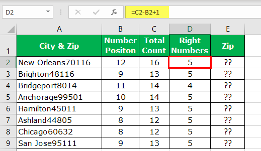
When we get the data, it follows a certain pattern, and having all the numbers at the end of the string is one of the patterns.
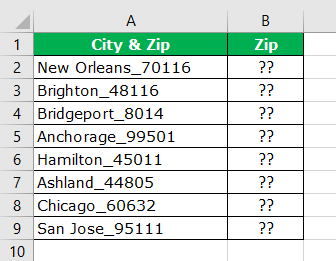
- For example, the city with its zip code below is a sample of the same.

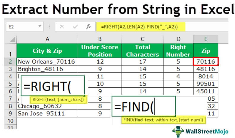
- We have the city name and zip code in the above example. In this case, we know we have to extract the zip code from the right-hand side of the string. But, we do not know exactly how many digits we need from the right-hand side of the string.
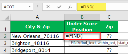
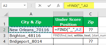
Before the numerical value starts, one of the common things is the underscore (_) character. So first, we need to identify the position of the underscore character. We can do it by using the FIND method. So, apply the FIND function in excel.

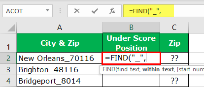
- What text do we need to find in the find_text argument? In this example, we need to find the position of the underscore, so enter the underscore in double quotes.

- The within_text is in which text we need to find the mentioned text, so select cell reference.

- The last argument is not required, so leave it as of now.

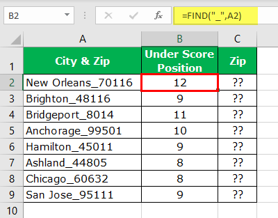
- So, we have got positions of underscore character for each cell. Next, we need to identify how many characters we have in the entire text. So, we must apply the LEN function in Excel to get the total length of the text value.

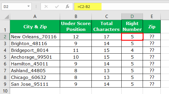
- Now, we have total characters and positions of underscore before the numerical value. Therefore, to supply the number of characters needed for the RIGHT function, we must minus the Total Characters with Underscore Position.

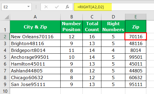
- Now, apply the RIGHT function in cell E2.

- So, like this, we can get the numbers from the right-hand side when we have a common letter before the number starts in the string value. Instead of having so many helper columns, we can apply the formula in a single cell.


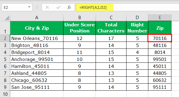
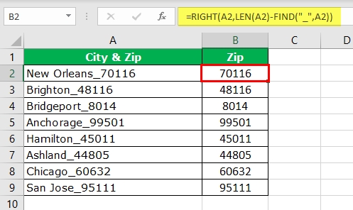
=RIGHT(A2,LEN(A2)-FIND(“_”,A2))
It will eliminate all the supporting columns and reduce the time drastically.
#2 – Extract Numbers From Right Side but Without Special Characters
Assume we have the same data, but this time we do not have any special character before the numerical value.
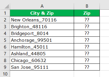
We have found a special character position in the previous example, but we do not have that luxury here. So, the formula below will find the “Numerical Position.”
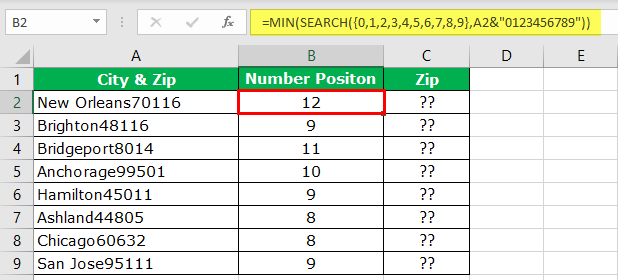
Please do not turn off your computer by looking at the formula. We will decode this for you.
For the SEARCH function in excelSearch function gives the position of a substring in a given string when we give a parameter of the position to search from. As a result, this formula requires three arguments. The first is the substring, the second is the string itself, and the last is the position to start the search.read more, we have supplied all the possible starting numbers of numbers, so the formula looks for the position of the numerical value. Since we have provided all the possible numbers to the array, the resulting arrays should contain the same numbers. Then, the MIN function in excelIn Excel, the MIN function is categorized as a statistical function. It finds and returns the minimum value from a given set of data/array.read more returns the smallest number among the two, so the formula reads below.
=MIN(SEARCH({0,1,2,3,4,5,6,7,8,9},A2&”0123456789″))
So, now we have the “Numerical Position.” But, first, let us find the total number of characters in the cell.
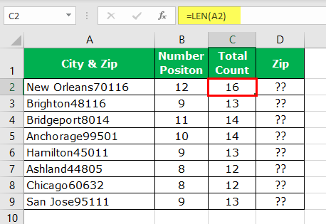
Consequently, it will return the total number of characters in the supplied cell value. Now, the “LEN” – position of the numerical value will return the number of characters required from the right side, so apply the formula to get the number of characters.
Now, we must apply the RIGHT function in excelRight function is a text function which gives the number of characters from the end from the string which is from right to left. For example, if we use this function as =RIGHT ( “ANAND”,2) this will give us ND as the result.read more to get only the numerical part from the string.
Let us combine the formula in a single cell to avoid multiple helper columns.
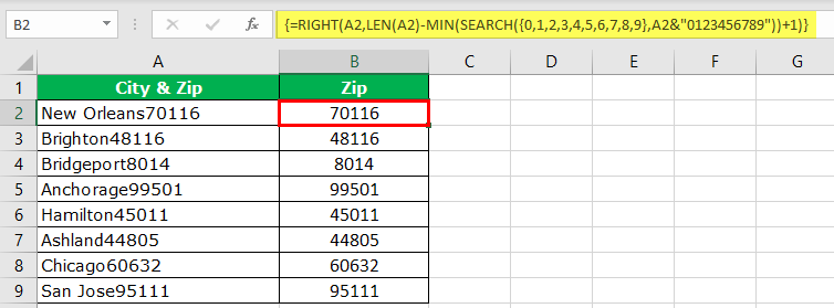
{=RIGHT(A2,LEN(A2)-MIN(SEARCH({0,1,2,3,4,5,6,7,8,9},A2&”0123456789″))+1)}
#3 – Extract Number From Any Position in Excel
We have seen from the RIGHT side extraction. But this is not the case with all the scenarios, so now we will see how to extract numbers from any string position in Excel.
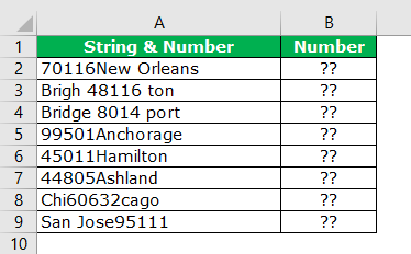
For this, we need to employ various functions of Excel. Below is the formula to extract the numbers from any string position.
=IF(SUM(LEN(A2)-LEN(SUBSTITUTE(A2, {“0″,”1″,”2″,”3″,”4″,”5″,”6″,”7″,”8″,”9”}, “”)))>0, SUMPRODUCT(MID(0&A2, LARGE(INDEX(ISNUMBER(–MID(A2,ROW(INDIRECT(“$1:$”&LEN(A2))),1))* ROW(INDIRECT(“$1:$”&LEN(A2))),0), ROW(INDIRECT(“$1:$”&LEN(A2))))+1,1) * 10^ROW(INDIRECT(“$1:$”&LEN(A2)))/10),””)
Recommended Articles
This article is a guide to Extract Number From String in Excel. We discussed the top 3 easy methods, step-by-step examples, and a downloadable Excel template. You may learn more about Excel from the following articles: –
- MID Function in Excel
- REPLACE Function in Excel
- Substring in Excel
- VBA String Functions
How to get the row or column number of the current cell or any other cell in Excel.
This tutorial covers important functions that allow you to do everything from alternate row and column shading to incrementing values at specified intervals and much more.
We will use the ROW and COLUMN function for this. Here is an example of the output from these functions.
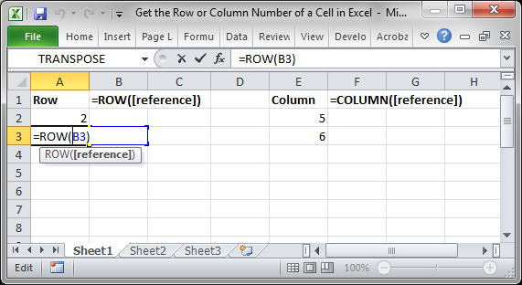
Though this doesn’t look like much, these functions allow for the creation of powerful formulas when combined with other functions. Now, let’s look at how to create them.
Get a Cell’s Row Number
Syntax
This function returns the number of the row that a particular cell is in.
If you leave the function empty, it will return the row number for the current cell in which this function has been placed.
If you put a cell reference within this function, it will return the row number for that cell reference.
This example would return 1 since cell A1 is in row 1. If it was =ROW(C24) the function would return the number 24 because cell C24 is in row 24.
Examples
Now that you know how this function works, it may seem rather useless. Here are links to two examples where this function is key.
Increment a Value Every X Number of Rows in Excel
Shade Every Other Row in Excel Quickly
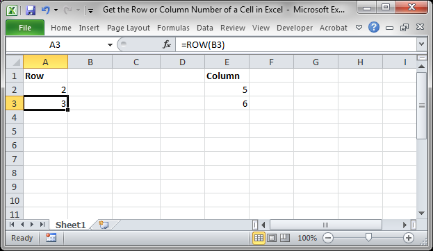
Get a Cell’s Column Number
Syntax
This function returns the number of the column that a particular cell is in. It counts from left to right, where A is 1 and B is 2 and so on.
If you leave the function empty, it will return the column number for the current cell in which this function has been placed.
If you put a cell reference within this function, it will return the column number for that cell reference.
This example would return 1 since cell A1 is in row 1. If it was =COLUMN (C24) the function would return the number 3 because cell C24 is in column number 3.
Examples
The COLUMN function works just like the ROW function does except that it works on columns, going left to right, whereas the ROW function works on rows, going up and down.
As such, almost every example where ROW is used could be converted to use COLUMN based on your needs.
Notes
The ROW and COLUMN functions are building blocks in that they help you create more complex formulas in Excel. Alone, these functions are pretty much worthless, but, if you can memorize them and keep them for later, you will start to find more and more uses for them when working in large data sets. The examples provided above in the ROW section cover only two of many different ways you can use these functions to create more powerful and helpful spreadsheets.
Similar Content on TeachExcel
Sum Values from Every X Number of Rows in Excel
Tutorial: Add values from every x number of rows in Excel. For instance, add together every other va…
Formulas to Remove First or Last Character from a Cell in Excel
Tutorial: Formulas that allow you to quickly and easily remove the first or last character from a ce…
Formula to Delete the First or Last Word from a Cell in Excel
Tutorial:
Excel formula to delete the first or last word from a cell.
You can copy and paste the fo…
Reverse the Contents of a Cell in Excel — UDF
Macro: Reverse cell contents with this free Excel UDF (user defined function). This will mir…
Excel Function to Remove All Text OR All Numbers from a Cell
Tutorial: How to create and use a function that removes all text or all numbers from a cell, whichev…
Get the First Word from a Cell in Excel
Tutorial: How to use a formula to get the first word from a cell in Excel. This works for a single c…