
If you have an Excel workbook that has hundreds of worksheets, and now you want to get a list of all the worksheet names, you can refer to this article. Here we will share 3 simple methods with you.
Sometimes, you may be required to generate a list of all worksheet names in an Excel workbook. If there are only few sheets, you can just use the Method 1 to list the sheet names manually. However, in the case that the Excel workbook contains a great number of worksheets, you had better use the latter 2 methods, which are much more efficient.
Method 1: Get List Manually
- First off, open the specific Excel workbook.
- Then, double click on a sheet’s name in sheet list at the bottom.
- Next, press “Ctrl + C” to copy the name.

- Later, create a text file.
- Then, press “Ctrl + V” to paste the sheet name.

- Now, in this way, you can copy each sheet’s name to the text file one by one.


Method 2: List with Formula
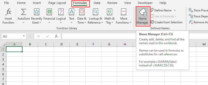
- At the outset, turn to “Formulas” tab and click the “Name Manager” button.
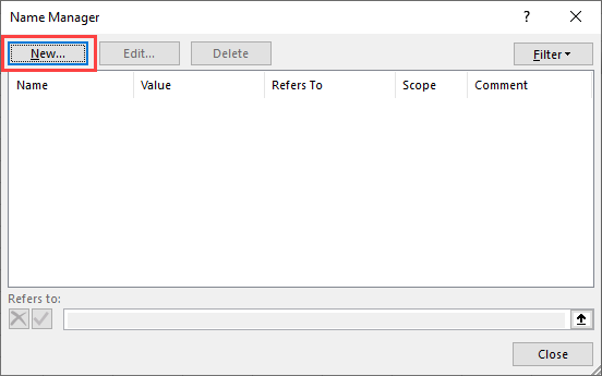
- Next, in popup window, click “New”.

- In the subsequent dialog box, enter “ListSheets” in the “Name” field.
- Later, in the “Refers to” field, input the following formula:

=REPLACE(GET.WORKBOOK(1),1,FIND("]",GET.WORKBOOK(1)),"")

- After that, click “OK” and “Close” to save this formula.
- Next, create a new worksheet in the current workbook.
- Then, enter “1” in Cell A1 and “2” in Cell A2.
- Afterwards, select the two cells and drag them down to input 2,3,4,5, etc. in Column A.

- Later, put the following formula in Cell B1.

=INDEX(ListSheets,A1)

- At once, the first sheet name will be input in Cell B1.
- Finally, just copy the formula down until you see the “#REF!” error.


Method 3: List via Excel VBA
- For a start, trigger Excel VBA editor according to “How to Run VBA Code in Your Excel“.
- Then, put the following code into a module or project.
Sub ListSheetNamesInNewWorkbook()
    Dim objNewWorkbook As Workbook
    Dim objNewWorksheet As Worksheet

    Set objNewWorkbook = Excel.Application.Workbooks.Add
    Set objNewWorksheet = objNewWorkbook.Sheets(1)

    For i = 1 To ThisWorkbook.Sheets.Count
        objNewWorksheet.Cells(i, 1) = i
        objNewWorksheet.Cells(i, 2) = ThisWorkbook.Sheets(i).Name
    Next i

    With objNewWorksheet
         .Rows(1).Insert
         .Cells(1, 1) = "INDEX"
         .Cells(1, 1).Font.Bold = True
         .Cells(1, 2) = "NAME"
         .Cells(1, 2).Font.Bold = True
         .Columns("A:B").AutoFit
    End With
End Sub

- Later, press “F5” to run this macro right now.
- At once, a new Excel workbook will show up, in which you can see the list of worksheet names of the source Excel workbook.


Comparison
| Advantages | Disadvantages | |
| Method 1 | Easy to operate | Too troublesome if there are a lot of worksheets |
| Method 2 | Easy to operate | Demands you to type the index first |
| Method 3 | Quick and convenient | Users should beware of the external malicious macros |
| Easy even for VBA newbies |
Excel Gets Corrupted
MS Excel is known to crash from time to time, thereby damaging the current files on saving. Therefore, it’s highly recommended to get hold of an external powerful Excel repair tool, such as DataNumen Outlook Repair. It’s because that self-recovery feature in Excel is proven to fail frequently.
Author Introduction:
Shirley Zhang is a data recovery expert in DataNumen, Inc., which is the world leader in data recovery technologies, including sql fix and outlook repair software products. For more information visit www.datanumen.com
This post will guide you how to get a list of all worksheet names in an excel workbook. How do I List the Sheet names with Formula in Excel. How to generate a list of all sheet tab names using Excel VBA Code.
Assuming that you have a workbook that has hundreds of worksheets and you want to get a list of all the worksheet names in the current workbook. And the below will introduce 3 methods with you.
Table of Contents
- Get All Worksheet Names Manually
- Get All Worksheet Names with Formula
- Get All Sheet Names with Excel VBA Macro
- Related Functions
Get All Worksheet Names Manually
If there are only few worksheets in your workbook, and you can get a list of all worksheet tab names by manually. Let’s see the below steps:
#1 open your workbook
#2 double click on the sheet’s name in the sheet tab. Press Ctrl + C shortcuts in your keyboard to copy the selected sheet.
#3 create a notepad file, and then press Ctrl +V to paste the sheet name.
#4 follow the above steps 2-3 to copy&paste all worksheet names into notepad file.
Get All Worksheet Names with Formula
You can also use a formula to get a list of all worksheet names with a formula. You can create a formula based on the LOOKUP function, the CHOOSE function, the INDEX function, the MID function, the FIND function and the ROWS function. Just do the following steps:
#1 go to FORMULAS tab, click Name Manager command under Defined Names group. The Name Manager dialog will open.
#2 click New… button to create a define name, type Sheets in the Name text box, and type the formula into the Refers to text box.
=GET.WORKBOOK(1)&T(NOW())
#3 Type the following formula into a blank cell and press Enter key in your keyboard, and then drag the autofill handle over others cells to get the rest sheet names.
=LOOKUP("xxxxx",CHOOSE({1,2},"",INDEX(MID(Sheets,FIND("]",Sheets)+1,255),ROWS(A$1:A1))))
You will see that all sheet names have been listed in the cells.
Get All Sheet Names with Excel VBA Macro
You can also use an Excel VBA Macro to quickly get a list of all worksheet tab names in your workbook. Just do the following steps:
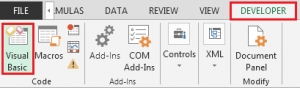
#1 open your excel workbook and then click on “Visual Basic” command under DEVELOPER Tab, or just press “ALT+F11” shortcut.

#2 then the “Visual Basic Editor” window will appear.
#3 click “Insert” ->”Module” to create a new module

#4 paste the below VBA code into the code window. Then clicking “Save” button.
Sub GetListOfAllSheets()
   Dim w As Worksheet
   Dim i As Integer
   i = 1
   Sheets("Sheet1").Range("A:A").Clear
   For Each w In Worksheets
       Sheets("Sheet1").Cells(i, 1) = w.Name
       i = i + 1
   Next w
End Sub
#5 back to the current worksheet, then run the above excel macro. Click Run button.
#6 Let’s see the result.
- Excel MID function
The Excel MID function returns a substring from a text string at the position that you specify.The syntax of the MID function is as below:= MID (text, start_num, num_chars)… - Excel LOOKUP function
The Excel LOOKUP function will search a value in a vector or array.The LOOKUP function is a build-in function in Microsoft Excel and it is categorized as a Lookup and Reference Function.The syntax of the LOOKUP function is as below:= LOOKUP (lookup_value, lookup_vector, [result_vector])… - Excel Choose Function
The Excel CHOOSE function returns a value from a list of values. The CHOOSE function is a build-in function in Microsoft Excel and it is categorized as a Lookup and Reference Function.The syntax of the CHOOSE function is as below:=CHOOSE (index_num, value1,[value2],…)… - Excel INDEX function
The Excel INDEX function returns a value from a table based on the index (row number and column number)The INDEX function is a build-in function in Microsoft Excel and it is categorized as a Lookup and Reference Function.The syntax of the INDEX function is as below:= INDEX (array, row_num,[column_num])… - Excel ROWS function
The Excel ROWS function returns the number of rows in a cell reference.The syntax of the ROWS function is as below:= ROWS(array)… - Excel FIND function
The Excel FIND function returns the position of the first text string (sub string) within another text string.The syntax of the FIND function is as below:= FIND(find_text, within_text,[start_num])
Содержание
- How can I get a list of all the sheets that are in a file on one sheet?
- 6 Answers 6
- Get sheet name only
- Related functions
- Summary
- Generic formula
- Explanation
- Workbook path
- TEXTAFTER function
- MID + FIND function
- How to Get the Sheet Name in Excel? Easy Formula
- Get Sheet Name Using the CELL Function
- Alternative Formula to Get Sheet Name (MID formula)
- Fetching Sheet Name and Adding Text to it
- List all Worksheet Names
- Get All Worksheet Names Manually
- Get All Worksheet Names with Formula
- Get All Sheet Names with Excel VBA Macro
- How To Get All Sheet Names From All Workbooks In A Folder
- The Setup
- Create a From Folder Query
- Filter on Excel Files
- Remove All Columns Not Needed
- Add a Custom Column
- Expand the Sheets Column
- Filter on the Sheet Kind
- Close and Load the Query
- Conclusions
How can I get a list of all the sheets that are in a file on one sheet?
Is there a way to find the names of all the sheets as a list?
I can find the sheet name of the sheet where the formula is placed in via the following formula:
This works for the sheet the formula is placed in. How can I get a list of all the sheets that are in a file on one sheet (let’s say in cell A1:A5 if I have 5 sheets)?
I would like to make it so when someone changes a sheet name the macro keeps working.
6 Answers 6
btw, in vba you can refer to worksheets by name or by object. See below, if you use the first method of referencing your worksheets it will always work with any name. 
I would keep a very hidden sheet with the formula you used referencing each sheet.
When the Workbook_NewSheet event fires a formula pointing to the new sheet is created:
- Create a sheet and give it the Code Name of shtNames .
- Give the sheet a tab name of SheetNames .
- In cell A1 of shtNames add a heading (I just used «Sheet List»).
- In Properties for the sheet change Visible to 2 — xlSheetVeryHidden.
You can only do this if there at least one visible sheet left.
- Add this code to the ThisWorkbook module:
Create a named range in the Name Manager:
- I called it SheetList .
- Use this formula:
=SheetNames!$A$2:INDEX(SheetNames!$A:$A,COUNTA(SheetNames!$A:$A))
You can then use SheetList as the source for Data Validation lists and list controls.
Two potential problems I haven’t looked at yet are rearranging the sheets and deleting the sheets.
so when someone changes a sheetname the macro keeps working
As @SNicolaou said though — use the sheet code name which the user can’t change and your code will carry on working no matter the sheet tab name.
Источник
Get sheet name only

Summary
To get the name of the current worksheet (i.e. current tab) you can use a formula based on the CELL function together with the TEXTAFTER function. In the example shown, the formula in E5 is:
The result is «September» the name of the current worksheet in the workbook shown. In older versions of Excel which do not provide the TEXTAFTER function, you can use an alternate formula based on the MID and FIND function. Both approaches are explained below.
Generic formula
Explanation
In this example, the goal is to return the name of the current worksheet (i.e. tab) in the current workbook with a formula. This is a simple problem in the latest version of Excel, which provides the TEXTAFTER function. In older versions of Excel, you can use an alternative formula based on the MID and FIND functions. Both formula options rely on the CELL function to get a full path to the current workbook. Read below for a full explanation.
Workbook path
The first step in this problem is to get the workbook path, which includes the workbook and worksheet name. This can be done with the CELL function like this:
With the info_type argument set to «filename», and reference set to cell A1 in the current worksheet, the result from CELL is a full path as a text string like this:
Notice the sheet name begins after the closing square bracket («]»). The problem now becomes how to extract the sheet name from the path? The best way to do this depends on your Excel version. Use the TEXTAFTER function if available. Otherwise, use the MID and FIND functions as explained below.
TEXTAFTER function
In Excel 365, the easiest option is to use the TEXTAFTER function with the CELL function like this:
The CELL function returns the full path to the current workbook as explained above, and this text string is delivered to TEXTAFTER as the text argument. Delimiter is set to «]» in order to retrieve only text that occurs after the closing square bracket («]»). In the example shown, the final result is «September» the name of the current worksheet in the workbook shown.
MID + FIND function
In older versions of Excel that do not offer the TEXTAFTER function, you can use the MID function with the FIND function to extract the sheet name:
The core of this formula is the MID function, which is used to extract text starting at a specific position in a text string. Working from the inside out, the first CELL function returns the full path to the current workbook to the MID function as the text argument:
We then need to tell MID where to start extracting text. To do this, we use the FIND function with a second call to the CELL function to locate the «]» character. We want MID to start extracting text after the «]» character, so we use the FIND function to get the position, then add 1:
The result from the above snippet is returned to the MID function as start_num. For the num_chars argument, we hard-code the number 255*. The MID function doesn’t care if the number of characters requested is larger than the length of the remaining text, it simply extracts all remaining text. The final result is «September» the name of the current worksheet in the workbook shown.
*Note: In Excel user interface, you can’t name a worksheet longer than 31 characters, but the file format itself permits worksheet names up to 255 characters, so this ensures the entire name is retrieved.
Источник
How to Get the Sheet Name in Excel? Easy Formula
When working with Excel spreadsheets, sometimes you may have a need to get the name of the worksheet.
While you can always manually enter the sheet name, it won’t update in case the sheet name is changed.
So if you want to get the sheet name, so that it automatically updates when the name is changed, you can use a simple formula in Excel.
In this tutorial, I will show you how to get the sheet name in Excel using a simple formula.
This Tutorial Covers:
Get Sheet Name Using the CELL Function
CELL function in Excel allows you to quickly get information about the cell in which the function is used.
This function also allows us to get the entire file name as a result of the formula.
Suppose I have an Excel workbook with the sheet name ‘Sales Data’
Below is the formula that I have used in any cells in the ‘Sales Data’ worksheet:

As you can see, it gave me the whole address of the file in which I am using this formula.
But I needed only the sheet name, not the whole file address,
Well, to get the sheet name only, we will have to use this formula along with some other text formulas, so that it can extract only the sheet name.
Below is the formula that will give you only the sheet name when you use it in any cell in that sheet:

The above formula will give us the sheet name in all scenarios. And the best part is that it would automatically update in case you change the sheet name or the file name.
Note that the CELL formula only works if you have saved the workbook. If you haven’t, then it would return a blank (as it has no idea what the workbook path is)
Wondering how this formula works? Let me explain!
The CELL formula gives us the whole workbook address along with the sheet name at the end.
One rule it would always follow is to have the sheet name after the square bracket (]).
Knowing this, we can find out the position of the square bracket, and then extract everything after it (which would be the sheet name)
And that’s exactly what this formula does.
The FIND part of the formula looks for ‘]’ and return it’s position (which is a number that denotes the number of characters after which the square bracket is found)
We use this position of the square bracket within the RIGHT formula to extract everything after that square bracket
One major issue with the CELL formula is that it’s dynamic. So if you use it in Sheet1 and then go to Sheet2, the formula in Sheet1 would update and show you the name as Sheet2 (despite the formula being on Sheet1). This happens as the CELL formula considers the cell in the active sheet and gives the name for that sheet, no matter where it is in the workbook. A workaround would be to hit the F9 key when you want to update the CELL formula in the active sheet. This will force a recalculation.
Alternative Formula to Get Sheet Name (MID formula)
There are many different ways to do the same thing in Excel. And in this case, there is another formula that works just as well.
Instead of the RIGHT function, it uses the MID function.
Below is the formula:
This formula works similarly to the RIGHT formula, where it first finds the position of the square bracket (using the FIND function).
It then uses the MID function to extract everything after the square bracket.
Fetching Sheet Name and Adding Text to it
If you’re building a dashboard, you may want to not just get the name of the worksheet, but also append a text before or after it.
For example, if you have a sheet name 2021, you may want to get the result as ‘Summary of 2021’ (and not just the sheet name).
This can easily be done by combining the formula we saw above with the text we want before it using the ampersand operator.
Below is the formula that will add the text ‘Summary of ‘ before the sheet name:

The ampersand operator (&) simply combines the text before the formula with the result of the formula. You can also use the CONCAT or CONCATENATE function instead of an ampersand.
Similarly, if you want to add any text after the formula, you can use the same ampersand logic (i.e., have the ampersand after the formula followed by the text that you want to append).
So these are two simple formulas that you can use to get the sheet name in Excel.
I hope you found this tutorial useful.
Other Excel tutorials you may also like:
Источник
List all Worksheet Names
This post will guide you how to get a list of all worksheet names in an excel workbook. How do I List the Sheet names with Formula in Excel. How to generate a list of all sheet tab names using Excel VBA Code.
Assuming that you have a workbook that has hundreds of worksheets and you want to get a list of all the worksheet names in the current workbook. And the below will introduce 3 methods with you.
Get All Worksheet Names Manually
If there are only few worksheets in your workbook, and you can get a list of all worksheet tab names by manually. Let’s see the below steps:
#1 open your workbook
#2 double click on the sheet’s name in the sheet tab. Press Ctrl + C shortcuts in your keyboard to copy the selected sheet.
#3 create a notepad file, and then press Ctrl +V to paste the sheet name.
#4 follow the above steps 2-3 to copy&paste all worksheet names into notepad file.
Get All Worksheet Names with Formula
You can also use a formula to get a list of all worksheet names with a formula. You can create a formula based on the LOOKUP function, the CHOOSE function, the INDEX function, the MID function, the FIND function and the ROWS function. Just do the following steps:
#1 go to FORMULAS tab, click Name Manager command under Defined Names group. The Name Manager dialog will open.
#2 click New… button to create a define name, type Sheets in the Name text box, and type the formula into the Refers to text box.
#3 Type the following formula into a blank cell and press Enter key in your keyboard, and then drag the autofill handle over others cells to get the rest sheet names.
You will see that all sheet names have been listed in the cells.
Get All Sheet Names with Excel VBA Macro
You can also use an Excel VBA Macro to quickly get a list of all worksheet tab names in your workbook. Just do the following steps:
#1 open your excel workbook and then click on “Visual Basic” command under DEVELOPER Tab, or just press “ALT+F11” shortcut.
#2 then the “Visual Basic Editor” window will appear.
#3 click “Insert” ->”Module” to create a new module
#4 paste the below VBA code into the code window. Then clicking “Save” button.
#5 back to the current worksheet, then run the above excel macro. Click Run button.
Источник
How To Get All Sheet Names From All Workbooks In A Folder
It’s a task I’ve had to do before. Get a list of all the sheet names in a workbook with 100+ sheets in it.
With a bit of VBA know-how, it can be done fairly quickly. Writing the code to loop through all the sheet objects in the active workbook and write them out to a sheet would only take a dozen lines of code.
What if you needed to this for all workbooks in a given folder? Hmm, a bit more code and it’s possible. You first need to loop through all the workbooks in a folder, then for each one loop through all the sheets and write the names out to a workbook. Ok, it’s getting a bit more complicated and there’s a bit more code involved.
Ok, now what if you want to do this for the folder and all subfolders that it contains? You’d have to write code to check if a folder has any subfolders, then loop through them and check each one of those to see if they themselves have any subfolders… and so on, and on until you don’t find any more subfolders. At each folder level, you also need to loop through all the files and get sheet names too.
Who wants to spend their time writing code? I don’t. That’s what makes power query so awesome. Many things that used to require coding in VBA to do, can now be done quickly without a bit of coding.
The Setup
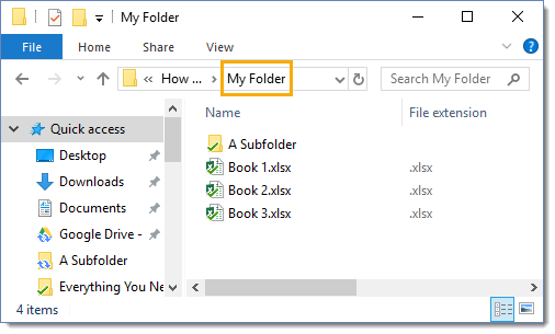
I’ve set up a folder called My Folder containing 3 Excel workbooks and one folder called A Subfolder (bravo John, very original name). Each workbook has a couple of sheets in them but is otherwise empty.
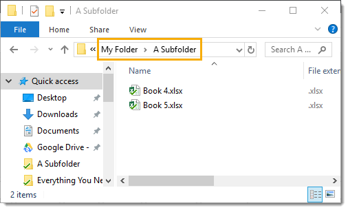
In the subfolder, I have a few more workbooks which are again empty apart from a couple of sheets.
Let’s see if we can get all the sheet names using Power Query.
Create a From Folder Query
First, we need to create a new From Folder query that targets our main folder.
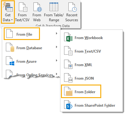
Go to the Data tab and press the Get Data button in the Get & Transform Data section. Then select From File and choose From Folder.

This will create a new query and you’ll be prompted to input the folder path of the main folder or you can browse to its location.
Next, a preview of the data will show up and you should see a list of file names along with other data about the files like extensions, dates, and paths. Press the Edit button to further edit these results.
Filter on Excel Files
It might be the case that some of the folders you have might contain different file types other than Excel files. Maybe you have some Word documents, pictures or powerpoint files in the folder or some of its subfolders. So we will need to first filter our query to only show us the Excel files in our folders.
In my case, I only have xlxs files in the folders so it’s not a vital step to get the query working now. It’s a good idea to add the filter in though, as this will prevent the query from breaking down the road if other types of files get added into the folder later.
It’s possible that an extension on a file appears all lower case or all upper case. We could have a .xlsx or .XLSX file extension, so we’ll need to incorporate this possibility into our filter since power query is case sensitive.
We may also want to allow for other Excel file extensions like .xls, .xlsm or .xlsb and their upper case versions as well.
![]()
To take care of extensions possibly being of lower or upper case, we will first transform them all into upper case. This way we will only have to account for the uppercase version in our filters. This will save a couple OR conditions in our filter step.
Right click on the Extension column heading in the data preview and select Transform and then UPPERCASE.
You can also access this from the Transform tab in the ribbon under the Format command found in the Text Column section.
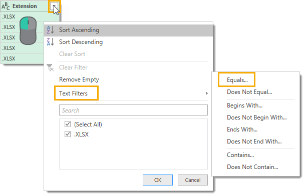
Now we can filter on the Extension column to make sure it only contains Excel workbooks. There’s only one item in the filter selection box now, so we’ll need to use the text filters to account for other options. Left click on the filter icon on the left hand side of the column heading and select Text Filters then choose the Equals option.
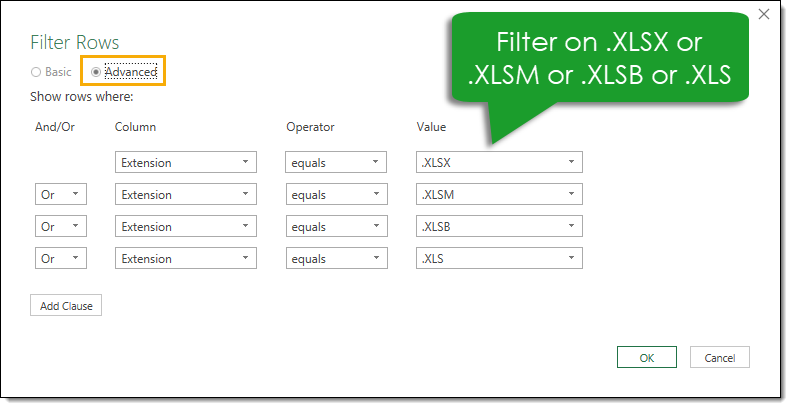
Navigate to the Advanced filter options and enter all the conditions. We’ll need to filter based on .XLSX or .XLSM or .XLSB or .XLS. Note that we need to include the period before the extension as this is included in the Extension field in our query results.
Now we have only the Excel files from our folders. If some other type of files gets added to the folders later, our query will filter them out and the query won’t fail with an error.
Remove All Columns Not Needed
There’s a lot of columns of data in here that we won’t be using and are just cluttering things up. We will only really be using the Name and Folder Path columns going forward, so we can remove the rest.

Select both the Name and Folder Path columns. This can be done by clicking on the first one then holding the Ctrl key and clicking on the second one. Now right click on the column heading and choose Remove Other Columns.
Add a Custom Column
Now that we have the path and file name of all the Excel workbooks in our folders and subfolders, we can use the Excel.Workbook function to get the sheet names from all these files. We’ll add in a custom column to use this function.
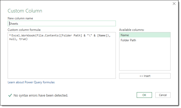
Go to the Add Column tab in the query editor ribbon and select Custom Column from the General section.
Now we can enter this formula and name the new column Sheets.
In this formula, we concatenate the file path with the file name to get the full address of the file. The File.Contents function will take this full address and return the binary contents of the file. The Excel.Workbook function then takes this content and returns a table representing the sheets in the given workbook.
Expand the Sheets Column
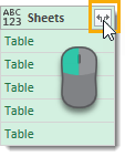
Now we have a column that contains a table for each row. The table in each row contains the sheets for the file listed in the row and we need to expand the tables to see all the sheet names.
Left click on the expand icon in the Sheets column and then choose Expand and press the OK button. We can also uncheck the Use original column name as prefix box here.
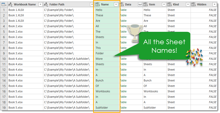
We now have all the sheet names.
Filter on the Sheet Kind
In our case, we only have Sheet in the Kind column because I was lazy and created workbooks that were empty apart from a couple sheets. It’s likely that your workbooks will have a lot of other things in them, so we’ll need to filter on this column to only keep sheets.
Create a Text Filter on the Kind column using the Equals option and filter on Sheet.
Close and Load the Query
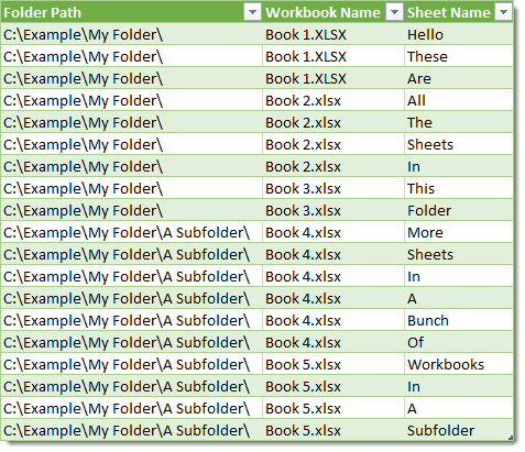
Before we close and load this into a table, I’m going to remove a couple of the columns I don’t need, and rename a few others and reorder them. Now it’s ready to close and load this query and we have the folder path, workbook name and all their sheet names from all the folders and subfolders. Wow, that’s awesome!
Conclusions
There are a lot of steps in the process, but once you start to become familiar with power query, most of them will become second nature. The hardest part of the process was writing a custom column formula with two power query functions. But I’d way rather do that than try and write some VBA that loops through all the folders and grabs the sheet names.
We were even able to keep track of which sheets were in which files and which folders. That would add another layer of things you needed to program into any VBA solution, and who need more work? That extra information just naturally came with the power query solution.
Источник
Is there a way to find the names of all the sheets as a list?
I can find the sheet name of the sheet where the formula is placed in via the following formula:
=RIGHT(CELL("filename";A1);LEN(CELL("filename";A1))-SEARCH("]";CELL("filename";A1);1))
This works for the sheet the formula is placed in. How can I get a list of all the sheets that are in a file on one sheet (let’s say in cell A1:A5 if I have 5 sheets)?
I would like to make it so when someone changes a sheet name the macro keeps working.
![]()
asked Dec 10, 2018 at 9:18
![]()
btw, in vba you can refer to worksheets by name or by object. See below, if you use the first method of referencing your worksheets it will always work with any name.
answered Dec 10, 2018 at 9:51
![]()
SNicolaouSNicolaou
5501 gold badge3 silver badges15 bronze badges
2
I would keep a very hidden sheet with the formula you used referencing each sheet.
When the Workbook_NewSheet event fires a formula pointing to the new sheet is created:
- Create a sheet and give it the Code Name of
shtNames.- Give the sheet a tab name of
SheetNames. - In cell
A1ofshtNamesadd a heading (I just used «Sheet List»). - In Properties for the sheet change Visible to 2 — xlSheetVeryHidden.
You can only do this if there at least one visible sheet left.
- Give the sheet a tab name of
- Add this code to the
ThisWorkbookmodule:
Private Sub Workbook_NewSheet(ByVal Sh As Object)

    With shtNames
        .Cells(.Rows.Count, 1).End(xlUp).Offset(1).Formula = _
            "=RIGHT(CELL(""filename"",'" & Sh.Name & "'!$A$1), " & _
            "LEN(CELL(""filename"",'" & Sh.Name & "'!$A$1))-" & _
            "FIND(""]"",CELL(""filename"",'" & Sh.Name & "'!$A$1),1))"
    End With

End Sub
Create a named range in the Name Manager:
- I called it
SheetList. - Use this formula:
=SheetNames!$A$2:INDEX(SheetNames!$A:$A,COUNTA(SheetNames!$A:$A))
You can then use SheetList as the source for Data Validation lists and list controls.
Two potential problems I haven’t looked at yet are rearranging the sheets and deleting the sheets.
so when someone changes a sheetname the macro keeps working
As @SNicolaou said though — use the sheet code name which the user can’t change and your code will carry on working no matter the sheet tab name.
answered Dec 10, 2018 at 10:43
![]()
@Mischa Urlings with the below code you get as a message in message box the following:
- Sheet Name
-
Sheet Position
Option Explicit

Sub test()

Dim ws As Worksheet
Dim str As String

For Each ws In ThisWorkbook.Worksheets
    str = str & vbNewLine & "Sheet named " & ws.Name & " located in position " & ws.Index & "."
Next

'Get the names in a list in message box
MsgBox str

End Sub
answered Dec 10, 2018 at 10:19
![]()
Error 1004Error 1004
7,8253 gold badges21 silver badges46 bronze badges
a VBA function like:
Function SheetName(ByVal Index As Long, Optional ByVal Book as Range) as String
    Application.Volatile
    If Book Is Nothing Then Set Book = Application.Caller
    SheetName=Book.Worksheet.Parent.Sheets(Index).Name
End Function
would return sheet names by index, like an Excel formula. Example:
=SheetName(1) 'returns "Sheet1"
=SheetName(3) 'returns "Sheet3"
Using optional range in another book, you can get other book sheet names:
=SheetName(1, [Some other book.xls]Sheet1!A1) 'returns "Sheet1"
=SheetName(2, [Some other book.xls]Sheet1!A1) 'returns "Sheet2"
answered Dec 10, 2018 at 9:32
![]()
LS_ᴅᴇᴠLS_ᴅᴇᴠ
10.8k1 gold badge22 silver badges46 bronze badges
3
Make a defined name(formulas, name manager) : named: YourSheetNames
in the field refersto you place:
=IF(NOW()>0,REPLACE(GET.WORKBOOK(1),1;FIND("]",GET.WORKBOOK(1)),""))
In your sheet you place in A1:A5:
=INDEX(YourSheetNames,ROW())
this wil give you (as long as calculation is set to xlautomatic) an actual list
answered Dec 10, 2018 at 9:28
![]()
EvREvR
3,3882 gold badges12 silver badges23 bronze badges
2
The following VBA macro function returns all worksheets names as an array:
Function GetWorksheets() As Variant

    Dim ws As Worksheet
    Dim x As Integer
    Dim WSArray As Variant
    ReDim WSArray(1 To Worksheets.Count)

    x = 1
    For Each ws In Worksheets
        'Sheets("Sheet1").Cells(x, 1) = ws.Name
        WSArray(x) = ws.Name
        x = x + 1
    Next ws

    'Output Array
    GetWorksheets = WSArray
End Function
After added to VBA Module, you can call it anywhere in a Workbook the same way you call a regular Excel Formula.


This VBA Function can be used as a more secure alternative to the following Excel 4.0 (XLM) macro:
=REPLACE(GET.WORKBOOK(1);1;FIND("]";GET.WORKBOOK(1));"")
answered Dec 8, 2022 at 6:03
![]()
When working with Excel spreadsheets, sometimes you may have a need to get the name of the worksheet.
While you can always manually enter the sheet name, it won’t update in case the sheet name is changed.
So if you want to get the sheet name, so that it automatically updates when the name is changed, you can use a simple formula in Excel.
In this tutorial, I will show you how to get the sheet name in Excel using a simple formula.
Get Sheet Name Using the CELL Function
CELL function in Excel allows you to quickly get information about the cell in which the function is used.
This function also allows us to get the entire file name as a result of the formula.
Suppose I have an Excel workbook with the sheet name ‘Sales Data’
Below is the formula that I have used in any cells in the ‘Sales Data’ worksheet:
=CELL("filename"))
As you can see, it gave me the whole address of the file in which I am using this formula.
But I needed only the sheet name, not the whole file address,
Well, to get the sheet name only, we will have to use this formula along with some other text formulas, so that it can extract only the sheet name.
Below is the formula that will give you only the sheet name when you use it in any cell in that sheet:
=RIGHT(CELL("filename"),LEN(CELL("filename"))-FIND("]",CELL("filename")))
The above formula will give us the sheet name in all scenarios. And the best part is that it would automatically update in case you change the sheet name or the file name.
Note that the CELL formula only works if you have saved the workbook. If you haven’t, then it would return a blank (as it has no idea what the workbook path is)
Wondering how this formula works? Let me explain!
The CELL formula gives us the whole workbook address along with the sheet name at the end.
One rule it would always follow is to have the sheet name after the square bracket (]).
Knowing this, we can find out the position of the square bracket, and then extract everything after it (which would be the sheet name)
And that’s exactly what this formula does.
The FIND part of the formula looks for ‘]’ and return it’s position (which is a number that denotes the number of characters after which the square bracket is found)
We use this position of the square bracket within the RIGHT formula to extract everything after that square bracket
One major issue with the CELL formula is that it’s dynamic. So if you use it in Sheet1 and then go to Sheet2, the formula in Sheet1 would update and show you the name as Sheet2 (despite the formula being on Sheet1). This happens as the CELL formula considers the cell in the active sheet and gives the name for that sheet, no matter where it is in the workbook. A workaround would be to hit the F9 key when you want to update the CELL formula in the active sheet. This will force a recalculation.
Alternative Formula to Get Sheet Name (MID formula)
There are many different ways to do the same thing in Excel. And in this case, there is another formula that works just as well.
Instead of the RIGHT function, it uses the MID function.
Below is the formula:
=MID(CELL("filename"),FIND("]",CELL("filename"))+1,255)
This formula works similarly to the RIGHT formula, where it first finds the position of the square bracket (using the FIND function).
It then uses the MID function to extract everything after the square bracket.
Fetching Sheet Name and Adding Text to it
If you’re building a dashboard, you may want to not just get the name of the worksheet, but also append a text before or after it.
For example, if you have a sheet name 2021, you may want to get the result as ‘Summary of 2021’ (and not just the sheet name).
This can easily be done by combining the formula we saw above with the text we want before it using the ampersand operator.
Below is the formula that will add the text ‘Summary of ‘ before the sheet name:
="Summary of "&RIGHT(CELL("filename"),LEN(CELL("filename"))-FIND("]",CELL("filename")))
The ampersand operator (&) simply combines the text before the formula with the result of the formula. You can also use the CONCAT or CONCATENATE function instead of an ampersand.
Similarly, if you want to add any text after the formula, you can use the same ampersand logic (i.e., have the ampersand after the formula followed by the text that you want to append).
So these are two simple formulas that you can use to get the sheet name in Excel.
I hope you found this tutorial useful.
Other Excel tutorials you may also like:
- How to Rename a Sheet in Excel (4 Easy Ways + Shortcut)
- How to Insert New Worksheet in Excel (Easy Shortcuts)
- How to Unhide Sheets in Excel (All In One Go)
- How to Sort Worksheets in Excel using VBA (alphabetically)
- Combine Data From Multiple Worksheets into a Single Worksheet in Excel
- How to Compare Two Excel Sheets
- How to Group Worksheets in Excel
Return to Excel Formulas List
Download Example Workbook
Download the example workbook
This tutorial demonstrates how to list the sheet names of a workbook with a formula in Excel.
List Sheet Names Using Named Range and Formula
There is no built-in function in Excel that can list all the worksheets in a workbook. Instead you have two options:
- Use a VBA Macro to list all sheets in the workbook
- Create a Formula to list all sheets
If you want to use a formula, follow these steps:
- Create a named range “Worksheets”
- Use a formula to list out all sheet names.
Create Name Range for Sheet Names
To create a Named Range for the sheet names, in the Excel Ribbon: Formulas > Name Manager > New
Type “Worksheets” in the Name Box:
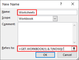
In the “Refers to” section of the dialog box, we will need to write the formula
=GET.WORKBOOK(1) & T(NOW())"This formula stores the names of all sheets (as an array in this format: “[workbook.xlsm].Overview”) in the workbook to the named range “Worksheets”.
The “GET.WORKBOOK” Function is a macro function, so your workbook has to be saved as a macro-enabled workbook (file format: .xlsm) for the sheet names to be updated each time the workbook is opened.
Note: When filling the Edit name dialog box, workbook should be selected as the scope of the name range.
Using Formula to List Sheet Names
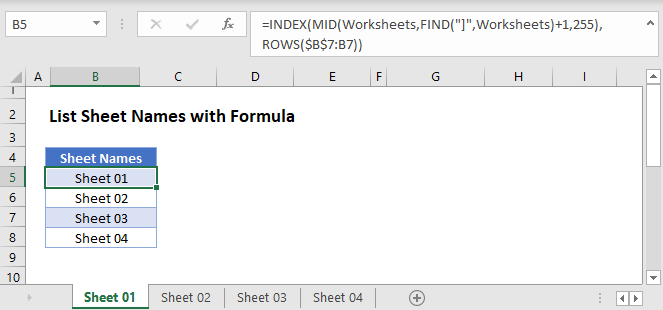
Now we use a formula to list the sheet names. We’ll need the INDEX, MID, FIND, and ROWS Functions:
=INDEX(MID(Worksheets,FIND("]",Worksheets)+1,255),ROWS($B$5:B5))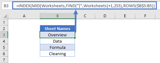
- The formula above takes the “Worksheets” array and displays each sheet name based on its position.
- The MID and FIND Functions extract the sheet names from the array (removing the workbook name).
- Then the INDEX and ROW Functions display each value in that array.
- Here, “Overview” is the first sheet in the workbooks and “Cleaning” is the last.
Click the link for more information on how the MID and FIND Functions get sheet names.
Alternate Method
You also have the option to create the list of sheet names within the Name Manager. Instead of
=GET.WORKBOOK(1) & T(NOW())set your “Refers to” field to
=REPLACE(GET.WORKBOOK(1),1,FIND("]",GET.WORKBOOK(1)),"")Now there’s no need for MID, FIND, and ROWS in your formula. Your named range is already made up of only sheet names.
Use this simpler INDEX formula to list the sheets:
=INDEX(SheetName,B3)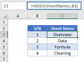
Explanation
The named range «sheetnames» is created with this code:
=GET.WORKBOOK(1)&T(NOW())
GET.WORKBOOK is a macro command that retrieves an array of sheet names in the current workbook. The resulting array looks like this:
{"[workbook.xlsm]Sheet1","[workbook.xlsm]Sheet2","[workbook.xlsm]Sheet3","[workbook.xlsm]Sheet4","[workbook.xlsm]Sheet5"}
A cryptic expression is concatenated to the result:
&T(NOW())
The purpose of this code is to force recalculation to pick up changes to sheet names. Because NOW is a volatile function, it recalculates with every worksheet change. The NOW function returns a numeric value representing date and time. The T function returns an empty string («») for numeric values, so the concatenation has no effect on values.
Back on the worksheet, cell B6 contains this formula copied down:
=INDEX(MID(sheetnames,FIND("]",sheetnames)+1,255),ROWS($B$5:B5))
Working from the inside out, the MID function is used to remove the worksheet names. The resulting array looks like this:
{"Sheet1","Sheet2","Sheet3","Sheet4","Sheet5"}
This goes into the INDEX function as «array». The ROW function uses an an expanding ranges to generate an incrementing row number. At each new row, INDEX returns the next array value. When there are no more sheet names to output, the formula will return a #REF error.
Note: because this formula relies on a macro command, you’ll need to save as a macro-enabled workbook if you want the formula to continue to update sheet names after the file is closed and re-opened. If you save as a normal worksheet, the sheetname code will be stripped.
How To Get Sheet Names Using VBA in Microsoft Excel
In case you want to find out a way which can get you all the names of the sheet that are visible i.e. not hidden.
In this article, we will learn how to get names of the visible sheets only, using VBA code.
Question): I have multiple sheets in one file & I have hidden the sheets which I do not want others to see; I want a code that will give me the name of all the visible sheets.
Let us consider we have 5 sheets & we intentionally hide a particular sheet.
To get name of the visible sheets, we need to follow the below steps:
- Click on Developer tab
- From Code group, select Visual Basic
Copy the below code in the standard module
Sub VisibleSheets()
Dim i As Integer, j As Integer: j = 1
Cells(1, 1).CurrentRegion.Cells.Clear
For i = 1 To Sheets.Count
If Sheets(i).Visible = -1 Then
Cells(j, 1) = Sheets(i).Name
j = j + 1
End If
Next
End Sub
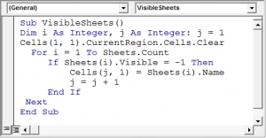
- First time when you run the code, you will get the names of all the sheets in current sheet in column A
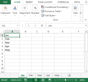
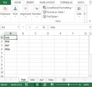
- If we hide Jan sheet then we will have following list of sheet names
In this way, we can get the name of all the visible sheets, using vba code.
![]()
Download — How to get sheet names with vba — xlsm