Генетические алгоритмы в excel

From The Developers of the Microsoft Excel Solver

Use Genetic Algorithms Easily for Optimization in Excel: Evolutionary Solver Works with Existing Solver Models, Handles Any Excel Formula, Finds Global Solutions

If Microsoft Excel is a familiar or productive tool for you, then you’ve come to the right place for genetic algorithms, evolutionary algorithms, or other methods for global optimization!  Frontline Systems developed the Solver in Excel for Microsoft.  Our Premium Solver products are upward compatible from the standard Excel Solver — your Solver models, and even your VBA code controlling the Solver, will work as-is.

You can use genetic algorithms for challenging problems that involve any Excel formulas or functions (even user-written functions).  With the same Premium Solver software, you can solve linear programming and nonlinear optimization models, and models with integer variables.  Define your optimization problem just once, in standard ‘Excel Solver’ form.  Then choose any of five built-in Solvers (including our Evolutionary Solver), or seven plug-in Solvers from a dropdown list, and click Solve.  That’s all there is to it!

If you register on Solver.com (it’s free), you can:

• Download a free 15-day Trial Version of any of our Excel Solver or SDK Solver products
• Download our Solver User Guides — learn more about genetic algorithms and other methods, the standard Excel Solver, Premium Solver, and how to build better optimization models
• Access «protected» Tech Support pages and downloadable example models

P. S.:  You don’t have to be an expert in optimization or «operations research.»  For more than a decade, thousands of users in Global 2000 companies have taken advantage of our advanced software and knowledgeable tech support to build and solve bigger and better models.

Premium Solver Platform

We offer Excel Solver upgrades for several types and sizes of optimization problems.  But our best-selling product is the Premium Solver Platform, in part because it can handle every type of problem up to certain size limits:

• Linear programming and quadratic programming problems up to 8,000 variables
• Conic and mixed-integer programming problems up to 2,000 variables
• Smooth nonlinear and global optimization problems (with our LSGRG Solver) up to 1,000 variables
• Non-smooth, global optimization problems (with our Evolutionary Solver) up to 1,000 variables

And you’ll want the Premium Solver Platform even if your problem is larger than these limits, because it is the base or «platform» that all of our larger-scale Solver Engines «plug into.»  If your problem grows in size, you can easily add one or more Solver Engines to the Premium Solver Platform at any time.The fastest way to learn more is to register for free, download and try out the Premium Solver Platform!  Or you can view more specific Premium Solver Platform Product Information.  For a quick summary, click here for our Excel Solver Product Comparison.  For pricing information, click on Excel Software and Support Prices.

Premium Solver

If the Premium Solver Platform is too much for your budget, and if you just need to solve a modest-size linear, mixed-integer, or smooth nonlinear model, you can use our Premium Solver Pro for less.  Premium Solver Pro includes our Simplex method Solver for linear programming, GRG Solver for nonlinear optimization, and Evolutionary Solver for non-smooth problems using genetic algorithms.

However, Premium Solver Prois not «expandable» to solve large-scale optimization problems.  All of our «plug-in» large-scale Solver Engines require the Premium Solver Platform, and the Polymorphic Spreadsheet Interpreter, available only in the Platform, plays a crucial role in the efficient solution of large-scale problems.

Click here for more specific Premium Solver Pro Product Information.  For a quick summary with problem size limits, click here for our Excel Solver Product Comparison.  To try out the Premium Solver, simply register and follow the link to download Excel products.

Solver Engines

If your problem is likely to exceed the size limits of the Premium Solver Platform for the type of optimization problem you want to solve, then you’ll want to choose a Solver Engine that handles larger-scale problems of that specific type.  For more information, click on Optional Plug-In Solver Engines.  If you register on Solver.com, you can download and try out all seven of our Solver Engines!

Even if your problem fits within the size limits of the Premium Solver Platform, you may find that you can obtain much faster solutions with Optional Plug-In Solver Engines.  It makes sense to choose a Solver Engine that uses algorithms or methods most efficient for your type of problem, especially if the problem is larger size.

Solver Engines range in price, depending on their features, speed and capacity — click on Excel Software and Support Prices for details.  For more information on Solver Engines for specific types of optimization problems, click on one of the links below:

• Linear and Quadratic Programming Problems
• Conic Optimization Problems
• Integer and Constraint Programming Problems
• Smooth Nonlinear Optimization Problems
• Global Optimization Problems
• Nonsmooth Optimization Problems

Note:  Every Frontline Systems Solver Product will handle problems with integer variables.  If your problem involves many such variables, however, you may find much faster solutions using the Solver Engines found through the link «Integer and Constraint Programming Problems» above.

Register for Download and Support Benefits

Register now! — it’s simple and free — so you can:

• Download a free 15-day Trial Version of any of our Excel Solver or SDK Solver products
• Download our Solver User Guides — learn more about the standard Excel Solver, Premium Solver, Risk Solver for Monte Carlo simulation, and how to build better optimization models
• Access «protected» Tech Support pages and downloadable example models

Just enter your name and email address, and optionally your company and phone, pick the closest «User Type,» and click the Register for Download button.  You can download immediately after registering, or return later anytime — just login with your email address — when you’re ready to try out our Excel Solver upgrades.

Problem

You’re an expert at using Solver for optimization but find it still can’t handle some troublesome problems, or you’d simply like to use an alternative optimization approach.

Solution

Genetic algorithms offer an alternative approach and are gaining popularity in optimization problem solving. You can use VBA to program your own genetic algorithm (or any other algorithm you can devise).

Discussion

This recipe is a little longer than the others and contains a lot of VBA code. If you’re not up to speed on using VBA, I recommend that you read Chapter 2 first.

Also, before getting into implementation details, I want to first explain some fundamental ideas behind genetic algorithms in case you aren’t already familiar with the concept.

Genetic Algorithm Fundamentals

Genetic algorithms are inspired by the biological evolutionary process. The basic idea for optimization problems is that solutions to a problem can be «bred» from a population of candidate solutions. Repeated breeding and survival of the fittest creates successive generations of offspring whose characteristics become more and more specialized or, to say it another way, which converge toward an optimum set of characteristics.

The trick with genetic algorithms, or rather one of the many tricks, is coming up with a way to encode the variables of a problem in a meaningful way that can be used to evolve a new set of values for the variables. A set of encoded variables is called a chromosome, a term obviously taken directly from the genetic algorithm’s biological roots. Chromosomes are comprised of genes , and genes represent the encoded variables for the problem.

In addition to devising a suitable structure for chromosomes, you have to devise a way to measure the fitness of each chromosome. In other words, you have to quantify how well the solution encoded in each chromosome solves, or optimizes, the problem you’re modeling. Fitness in this sense is directly related to the objective function of the problem.

The next big question that arises when developing a genetic algorithm is how to breed, or combine, chromosomes to generate successive populations in order to evolve a solution.

The way a genetic algorithm works is that you create an initial population of randomly generated chromosomes. The data encoded in these chromosomes will almost certainly not solve your problem well at all. The idea is to pick the fittest ones of this bunch and breed them to create a new population. You decide how chromosomes are bred. Most algorithms use some sort of crossover function, where you simply swap the genes between two parent chromosomes. For example, you might take the first half from the mommy chromosome and the second half from the daddy chromosome. Other practitioners take every other gene from the mommy and daddy. It’s really up to you and depends a lot on how you encoded your chromosomes in the first place.

Once a new population has been bred, it replaces the older generation. The new population is then evaluated for fitnessthat is, how well each new chromosome solves your problem. Next, a new set of fit parents are selected and used to generate a whole new population of offspring. This process repeats over many generations until the bred chromosomes converge on an optimal solution to the problem.

Naturally, there’s more to this than meets the eye. One big issue is what to do if you start with an initial, randomly selected population that is just terrible in that it very poorly satisfies the problem you’re trying to solve. If you breed with only these chromosomes, you’re left with a limited gene pool and almost surely no chance of finding a globally optimum solution.

To introduce new genetic material , in genetic algorithm lingo, you need to mutate the genes of offspring chromosomes. These mutations are random and provide opportunities for new characteristics to be introduced into the gene pool. Here again, there are many ways in which you may mutate a chromosome. A simple and common approach is to randomly select a gene and change it to some other randomly selected value. If it’s a bad mutation, one that produces poor results or an unfit chromosome, it will be purged through the selection and evolution process. On the other hand, if it’s a good mutation, it will be retained and passed along to subsequent generations. This is a key element of genetic algorithms, and we’ll talk more about it shortly when I get to some implementation details.

Given this basic description of genetic algorithms, it’s clear there’s a great deal of leeway available for formulating a genetic algorithm. There is no single genetic algorithm, and you are free to devise one that is well suited to the problem with which you are dealing.

Developing genetic algorithms seems, to me, to consist of a little theory and a lot of voodoo. I like them because the basic concept is simple and you have so much creative leeway in formulating an approach to a given problem. Plus, they work! At the same time, you can treat certain aspects of them in a rigorous theoretical manner. If you’re interested in the theory, I encourage you to check out Melanie Mitchell’s Introduction to Genetic Algorithms (MIT Press). There’s absolutely no source code in that book, but it covers the theory and a lot of history behind genetic algorithms.

The genetic algorithm I’ll show in this recipe is based on the concepts discussed here, but it’s tailored to solve a specific problem. The problem I’ll show you how to solve is the same troublesome function discussed in Recipe 13.4. If you have not already read Recipe 13.4, go back and have a look at it now to become familiar with the function we’re dealing with here.

Chromosome class

The first step in creating our Frankenstein’s monster is to create a chromosome class. The encoding for this chromosome is simple since there are only two variables to change, x and y.

To create this class, which we’ll call Chromosome, open the VBA editor window and create a new class module named Chromosome using the techniques I showed you in Recipe 2.14 in Chapter 2.

Once you’ve created the Chromosome class module, go ahead and add the properties shown here in Example 13-2.

Example 13-2. Chromosome properties

Public x As Double
Public y As Double
Public Z As Double
Public MaxX As Double
Public MinX As Double
Public MaxY As Double
Public MinY As Double
Public MutationRate As Double
Public FitnessScore As Double

The first three properties are x, y, and z. The genes in this chromosome are x and y. My encoding here is simple. The genes x and y are simply properties of the Chromosome class. Historically, many genetic algorithms use bit strings or some other low-level programming device to encode the problem variables. I personally like to use object properties or structures, depending on the language I’m using. I simply find them easier to deal with in code. But that’s just my preference.

The next four properties store the x and y bounds for the problem. Genes will be randomly selected within the range defined by these upper and lower bounds.

The second to last property, MutationRate, is very important. It specifies the probability of a chromosome mutating as described earlier. This value should be tuned to achieve acceptable results. Many researchers use a value of 0.001. I’ve played with it for this example and find that any mutation rate between 0.001 and 0.01 seems to yield good results. If the mutation rate is too low, then new genetic material is introduced at a very slow rate. This means that it could take a long time for the population to converge toward an optimum solution. On the other hand, if you set the mutation rate too high, you may never converge at all, because even fit chromosomes will mutate, possibly destroying their superior fitness.

The final property required for this problem is FitnessScore. This property stores a value that is used to rank the chromosomes according to their fitness. I’ll discuss how we actually measure fitness shortly. That’s it for Chromosome properties. Now I’ll show you all the methods required for this class.

The Class_Initialize method shown in Example 13-3 is the constructor, or initializing subroutine, for the Chromosome class. This subroutine is automatically called by VBA when a Chromosome object is created. I’m using it here to set the properties to default values.

Example 13-3. Initialize method

Private Sub Class_Initialize( )
 MutationRate = 0.05
 MaxX = 5
 MinX = -5
 MaxY = 5
 MinY = -5

 x = (MaxX - MinX + 1) * Rnd + MinX
 y = (MaxY - MinY + 1) * Rnd + MinY

 EvaluateZ

End Sub

I set the mutation rate to 0.05 by default, but as you’ll see later, this gets overridden with a value supplied through a spreadsheet cell. The bounds on x and y are set to -5 and 5. The next two lines generate random values for x and y within the default bounds and store these values in the x and y properties. Remember, these are the chromosome’s genes. Finally, the method EvaluateZ is called to calculate z using the function we’re trying to optimize, the one shown in Recipe 13.4. EvaluateZ is shown in Example 13-4.

Example 13-4. EvaluateZ method

Public Sub EvaluateZ( )
 Z = (1 - Cos(x * x + y * y) / (x * x + y * y + 0.5)) * 1.25
End Sub

EvaluateZ simply computes Z given the current values stored in x and y. I’ll show you later how Z is used to evaluate the fitness of the chromosome.

We need a method for Chromosome that mutates its genes given the mutation rate stored in the MutationRate property. The Mutate method shown in Example 13-5 is one I devised for this purpose.

Example 13-5. Mutate method

Public Sub Mutate( )
 Dim num As Double

 num = Rnd

 If num < MutationRate Then
 num = Rnd
 If num < 0.5 Then
 x = (MaxX - MinX + 1) * Rnd + MinX
 Else
 y = (MaxY - MinY + 1) * Rnd + MinY
 End If
 End If
End Sub

The first action performed in Mutate is the generation of a random number between 0 and 1. I used VBA’s Rnd function for this purpose and stored the value in the local variable num. The subsequent If statement compares num to the mutation rate. If num is less than MutationRate, then you need to mutate the chromosome; otherwise, don’t do anything with it.

If you do indeed need to mutate the chromosome, then Mutate generates another random number. If this number is less than 50, then the x gene is mutated; otherwise, the y gene is mutated. This scheme gives each gene a 50 percent chance of being mutated.

Mutating either gene is accomplished by simply generating a new random number for the gene between the bounds stored in the x or y bounds properties.

Example 13-6 shows another required method, the Mate method.

Example 13-6. Mate method

Public Sub Mate(mom As Chromosome, dad As Chromosome)
 ' Take average as crossover function
 x = (mom.x + dad.x) / 2
 y = (mom.y + dad.y) / 2

 ' Mutate the result
 Mutate
End Sub

As its name implies, this method takes two chromosomes and combines them in such a way as to yield an offspring chromosome that consists of some combination of its parents’ genes.

I played around with two different mating approaches for this example. First, I tried simply taking an x from dad and a y from mom to create the offspring. That worked OK, but I thought a better approach might be to simply average the x and y values, respectively, obtained from both mom and dad. After many trials, I think the averaging approach is better. It seems to converge faster to an optimum. (I’ll leave the reason why for someone else to figure out.)

After the offspring chromosome’s genes are computed, Mate calls Mutate to mutate the offspring.

The final method for this class is Copy. It’s a utility method that simply copies the properties of a given chromosome into the calling chromosome. Example 13-7 shows the Copy method.

Example 13-7. Copy method

Public Sub Copy(dup As Chromosome)
 x = dup.x
 y = dup.y
 Z = dup.Z
 MaxX = dup.MaxX
 MinX = dup.MinX
 MaxY = dup.MaxY
 MinY = dup.MinY
 MutationRate = dup.MutationRate
 FitnessScore = dup.FitnessScore
End Sub

That’s it for the Chromosome class. In the next section, I show you how to actually use this class.

Genetic optimization

Figure 13-19 shows the spreadsheet I set up for this example.

I set this up so you need only supply two parameters to the genetic algorithm. First, you must supply a limit on the number of generations evolved. Second, you must supply the mutation rate. These two values are contained in cells G1 and G2, respectively.

The Current Generation value shown in cell G4 is informational. As the genetic algorithm runs, it will display the current generation in this cell so you can track its progress. Further, the entire population of chromosomes for each generation is echoed back to this spreadsheet starting in cells A1, B1, and C1. This allows you to see how the populations evolve as the genetic algorithm does its thing.

Figure 13-19. Genetic algorithm spreadsheet

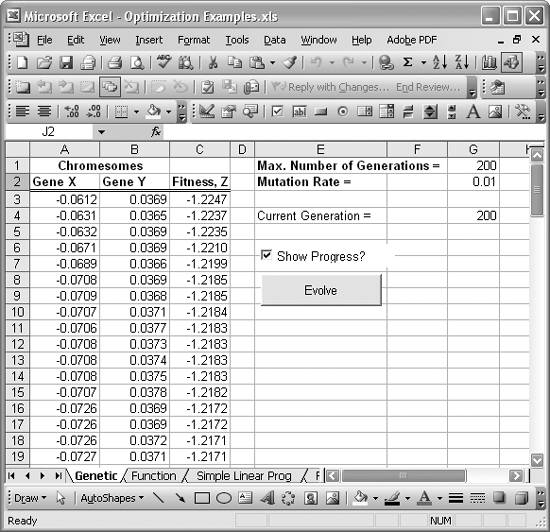
You’ll notice the «Show Progress?» checkbox on the spreadsheet just above the Evolve button. This checkbox is another ActiveX control available from the Control Toolbox toolbar (see Recipe 9.3 for more on the Control Toolbox).

You add a checkbox control just as you add a button control, as I’ve shown in other recipes throughout this book. Simply click the checkbox icon on the Control Toolbar and then click anywhere in your spreadsheet where you’d like the control located. While in design mode, you can right-click on the checkbox control and select Properties from the pop-up menu to display the control’s Properties window. As with button controls, you can change the name of the control, the caption displayed on the control, and many other attributes. I changed the caption to «Show Progress?» for this checkbox.

Checkbox controls have a value property that can be either true or false. When this value is true, the checkbox is checked. When it’s false, the checkbox is not checked. When a user clicks the checkbox, checking and unchecking it, the value property is changed accordingly. This allows you to programmatically inspect the value property to determine the state of the checkbox. I use it here to determine whether to update the spreadsheet with the status of each evolution as the genetic algorithm runs. Displaying the progress is certainly informative, but it is a lot slower; therefore, if you want the algorithm to run faster, you can uncheck the progress checkbox.

You can also associate code with a checkbox: the code will get executed when the user clicks on the checkbox. This is achieved in a manner similar to the way in which you associate code with a button, as discussed in Chapter 9.

The Evolve button allows you to start the genetic algorithm. I added this button using the same techniques I showed you in Chapter 9. The click event handler for this button is shown in Example 13-9; but, before I explain what it does, I want to go over some global variables required for the genetic algorithm. Example 13-8 shows these global variables.

Example 13-8. Global variables

Const PopulationSize As Integer = 100

Dim MaxGenerations As Integer
Dim MutationRate As Double
Dim CurrentGeneration(1 To PopulationSize) As Chromosome
Dim Offspring(1 To PopulationSize) As Chromosome
Dim SumFitnessScores As Double

The first line in Example 13-8 isn’t really a variableit’s a constant. The constant PopulationSize is an integer value that I set to 100. This means the initial and all subsequent chromosome populations will consist of 100 chromosomes. This is also a tunable value. If you set this too low, then the population won’t be diverse enough, and convergence to an optimum solution could be slow or unsuccessful. If it’s too high, the algorithm will run more slowly. 100 seemed like a good size for this problem. I tried a population size as low as 10 and as high as 200. In the former case, convergence was poor; in the latter case it was slower and no more accurate than a size of 100. So I stuck with 100.

The next five lines are actual variable declarations. These variables have module-level scope, so any function or subroutine in the same code module has access to them. Each variable is described in the following list:

MaxGenerations

MaxGenerations is an integer variable representing the limit on the number of generations to evolve. This value is extracted from spreadsheet cell G1.

MutationRate

MutationRate represents the probability of mutation as discussed earlier. Its value is extracted from spreadsheet cell G2.

CurrentGeneration

CurrentGeneration is an array of Chromosome objects. The size of this array is PopulationSize. This array represents the entire population of Chromosomes comprising the current generation.

Offspring

Offspring is another array of Chromosome objects. Its size is also PopulationSize. This array is used to store offspring chromosomes bred from the current generation. After all offspring are created, they replace the current generation, becoming the new CurrentGeneration.

SumFitnessScores

SumFitnessScores is a Double variable. It’s used to store the sum of fitness scores for all chromosomes in the current generation. Its value is used in a roulette wheel selection process that I’ll show you later.

Now, let’s get back to the click event handler for the Evolve button. The handler is shown in Example 13-9.

Example 13-9. Evolve button’s click event handler

Private Sub EvolveButton_Click( )
 Dim i As Integer

 Application.ScreenUpdating = ShowProgressCheckBox.Value

 Randomize

 MaxGenerations = Worksheets("Genetic").Range("MaxGenerations")
 MutationRate = Worksheets("Genetic").Range("MutationRate")

 For i = 1 To PopulationSize
 Set CurrentGeneration(i) = New Chromosome
 Set Offspring(i) = New Chromosome

 CurrentGeneration(i).MutationRate = MutationRate
 Next

 DoGeneticAlgorithm

 Application.ScreenUpdating = True
 Application.ActiveWorkbook.Save

End Sub

This subroutine is responsible for initializing and kicking off the genetic algorithm. After creating a local counter variable, i, the subroutine sets the status of screen updating to the value represented in the «Show Progress?» checkbox. The line Application.ScreenUpdating = ShowProgressCheckBox.Value takes care of that task. If the value property for the progress checkbox is true (indicating it’s checked) then screen updating will occur; otherwise, it won’t.

The next line of code simply initializes VBA’s random number generator with a call to Randomize. Next, the values for MaxGenerations and MutationRate are extracted from cells G1 and G2 in the spreadsheet. I named these two cells MaxGenerations and MutationRate, respectively (see Recipe 1.14 to learn how to name cells).

The For loop that comes next is responsible for creating the two required populations of Chromosome objects. Remember, the array declarations for CurrentGeneration and Offspring don’t actually create the Chromosome object. You have to use the Set and New statements as shown in Example 13-9 (and as discussed in Recipe 2.14) to create memory for the objects, initialize them, and assign them to the arrays.

After the arrays are taken care of, the mutation rate property for the current generation of chromosomes is set to the value provided in cell G2 and stored in the variable MutationRate.

After the For loop, a call is made to DoGeneticAlgorithm, which, as its name implies, executes the genetic algorithm. This subroutine is shown in Example 13-10. Before getting there, let me just say that the last two lines of code in Example 13-9 are responsible for turning screen updating back on and saving the workbook. Now, on to DoGeneticAlgorithm.

Example 13-10. DoGeneticAlgorithm subroutine

Public Sub DoGeneticAlgorithm( )
 Dim i As Integer
 Dim Generation As Integer
 Dim mom As Integer
 Dim dad As Integer

 Generation = 0
 EvaluteFitness
 DisplayResults

 Do While (Generation <= MaxGenerations)
 Worksheets("Genetic").Range("Generation") = Generation

 For i = 1 To PopulationSize
 mom = SelectChromosome
 dad = SelectChromosome
 Offspring(i).Mate CurrentGeneration(mom), CurrentGeneration(dad)
 Next

 For i = 1 To PopulationSize
 CurrentGeneration(i).Copy Offspring(i)
 Next

 Generation = Generation + 1
 EvaluteFitness
 DisplayResults
 Loop

 ' Sort the results:
 Range("A3:C102").Select
 Selection.Sort Key1:=Range("C3"), Order1:=xlAscending, Header:=xlGuess, _
 OrderCustom:=1, MatchCase:=False, Orientation:=xlTopToBottom, _
 DataOption1:=xlSortNormal
End Sub

DoGeneticAlgorithm requires four local variables. i is simply a counter variable used to loop over array elements. Generation is a counter variable used to keep track of the number of generations evolved. This value gets echoed back to the spreadsheet in cell G4. mom and dad are integers used to store indices to array elements in CurrentGeneration that represent two chromosomes selected for breeding.

With the local variables taken care of, DoGeneticAlgorithm initializes a few things. Generation is set to 0, and calls to EvaluateFitness and DisplayResults are made. EvaluateFitness updates the fitness scores for the chromosomes in the current generation, and DisplayResults displays the current generation’s genes and z-value in the spreadsheet. We’ll come back to the details of these two subroutines later.

DoGeneticAlgorithm next enters a Do While loop. This loop will repeat until the number of generations evolved reaches the limit stored in MaxGenerations. It is within this Do While loop that the evolution of a solution takes place.

The first action taken in this loop is simply to display the current generation number in the spreadsheet. Next, a For loop is encountered; it is responsible for selecting candidate chromosomes from the current generation and breeding them to create the new offspring population.

The integers mom and dad are selected via calls to a function called SelectChromosome. SelectChromosome selects candidates from the current generation, where the probability of selecting any individual chromosome is proportional to the chromosome’s fitness score. I’ll show you the details later. For now, just know that this is a survival-of-the-fittest selection process.

After two parents are selected, they are mated by calling the offspring Chromosome’s Mate method. Here’s the line of code that calls the Mate method:

 Offspring(i). Mate CurrentGeneration(mom), CurrentGeneration(dad)

This line calls the Mate method of Offspring(i), which is the ith Chromosome stored in the Offspring array. Mate requires two arguments, a mom and a dad Chromosome. These arguments are CurrentGeneration(mom) and CurrentGeneration(dad). Notice that there are no parentheses around these arguments, unlike when you make a function call or procedure call in most other languages. If you put parentheses around these arguments, VBA will return an error.

When this For loop is finished, Offspring will contain an entirely new population of chromosomes. The next task is to make this new population the CurrentGeneration. This task is achieved in the next For loop, which calls the Copy method for each chromosome in CurrentGeneration where the corresponding chromosome (based on the array index) in the Offspring array is passed as the chromosome to copy.

After all the chromosomes have been copied, the new population stored in CurrentGeneration is updated. First, the generation counter is incremented by 1. Then a call to EvaluateFitness is made to update the fitness scores for the new population. Finally, DisplayResults is called to display the current population in the spreadsheet.

At this point, execution goes back to the beginning of the Do While loop and repeats until the maximum number of generations has been reached. When that occurs, the last few lines of code in Example 13-10 are executed.

As the comment suggests, these lines sort the population displayed in cells A3 to C102 in the spreadsheet. This population represents the fittest population at the end of the evolution process. Not all of the chromosomes displayed in this list are the most fit and some are more fit than others. So to see which are the fittest, I sort the list to display the chromosomes in order from the fittest down to the least fit. This way you need only look at the uppermost values in the spreadsheet to see the results.

Now let’s take a look at the subroutine EvaluateFitness. As I mentioned earlier, this subroutine is responsible for assessing the fitness of each chromosome in the current population. EvaluateFitness first computes the z-value for each chromosome and then gives each chromosome a fitness score based on its z-value relative to the other z-values in the population. Remember, we’re trying to minimize z for the objective function; therefore, a lower z-value is better. So any chromosome whose genes (x and y) yield a lower z-value is more fit than a chromosome whose genes yield a higher z-value. We want these fitter chromosomes to reproduce so they’ll get a higher fitness score. Example 13-11 shows how I constructed EvaluteFitness.

Example 13-11. EvaluteFitness subroutine

Public Sub EvaluteFitness( )
 Dim i As Integer
 Dim MinZ As Double
 Dim MaxZ As Double

 CurrentGeneration(1).EvaluteZ
 MinZ = CurrentGeneration(1).Z
 MaxZ = CurrentGeneration(1).Z

 For i = 2 To PopulationSize
 CurrentGeneration(i).EvaluteZ
 If CurrentGeneration(i).Z > MaxZ Then
 MaxZ = CurrentGeneration(i).Z
 End If
 If CurrentGeneration(i).Z < MinZ Then
 MinZ = CurrentGeneration(i).Z
 End If
 Next

 SumFitnessScores = 0
 For i = 1 To PopulationSize
 CurrentGeneration(i).FitnessScore = 1 - _
 (CurrentGeneration(i).Z - MinZ) / (MaxZ - MinZ)

 SumFitnessScores = SumFitnessScores + CurrentGeneration(i).FitnessScore
 Next
End Sub

EvaluateFitness first declares a few local variables. Here again, i is simply a counter variable. MinZ and MaxZ are used to store the minimum and maximum z-values found in the current population. They represent the range of z-values for the population. They are initialized to the z-value for the first chromosome in the population. Then a For loop iterates over all remaining chromosomes in the current population. Within the For loop, each chromosome’s z-value is computed and compared to the minimum and maximum z-values stored in MinZ and MaxZ. If the chromosome’s z-value is higher or lower than the currently stored range, the range gets updated accordingly. By the time this For loop ends, MinZ and MaxZ will contain the range for the entire population.

Before the subroutine enters the next For loop, it sets SumFitnessScores to 0. Within the next For loop, SumFitnessScores will tally all of the fitness scores for every chromosome in the population.

The next For loop iterates over the entire current population, computing a fitness score for each chromosome. The formula I came up with for the fitness score is:

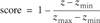
where zmin and zmax represent MinZ and MaxZ, respectively.

This formula gives the chromosome with the highest z-value a fitness score of 1 and the chromosome with the lowest z-value a fitness score of 0. All other chromosomes will have a score somewhere between 0 and 1. As I mentioned earlier, SumFitnessScores computes a running total of these fitness scores.

That’s it for the fitness score subroutine. Now let’s turn our attention to the function responsible for selecting the fittest chromosomes, based on their fitness scores. The function I wrote for this task is called SelectChromosome and is shown in Example 13-12.

Example 13-12. SelectChromosome function

Public Function SelectChromosome( ) As Integer
 Dim FitnessValue As Double
 Dim FitnessTotal As Double
 Dim i As Integer
 Dim Selection As Integer
 Dim continue As Boolean

 FitnessValue = Rnd * SumFitnessScores
 FitnessTotal = 0
 continue = True

 i = 1
 Do While (i <= PopulationSize) And (continue = True)
 FitnessTotal = FitnessTotal + CurrentGeneration(i).FitnessScore

 If FitnessTotal > FitnessValue Then
 Selection = i
 continue = False
 End If
 i = i + 1
 Loop
 SelectChromosome = Selection
End Function

This function selects chromosomes using a standard roulette wheel algorithm. The idea is to select chromosomes with a probability of selection proportional to the chromosomes’ fitness scores. Chromosomes with the highest fitness scores have greater probabilities of being selected, while those with lower scores have lower probabilities of being selected.

SelectChromosome implements the algorithm as follows: a random number between 0 and 1 is obtained and multiplied by the sum of all fitness scores. The result is stored in the variable FitnessValue. Next, a Do While loop is entered to iterate over the current population. During each iteration an accumulation variable, FitnessTotal, accumulates the fitness scores for each chromosome. When this FitnessTotal exceeds the randomly obtained FitnessValue, we have a selection. The chromosome whose fitness score tipped FitnessTotal over FitnessValue is the chromosome to select, and its index gets returned by SelectChromosome.

That’s pretty much it for the genetic algorithm portion of the code. The remaining function I want to show is DisplayResults. As mentioned earlier, it simply populates the spreadsheet (cells A3 through C102) with chromosome data for the current population. Example 13-13 shows the subroutine.

Example 13-13. DisplayResults subroutine

Public Sub DisplayResults( )
 Dim i As Integer
 Dim r As Integer

 r = 3
 For i = 1 To PopulationSize
 With Worksheets("Genetic")
 .Cells(r, 1) = CurrentGeneration(i).x
 .Cells(r, 2) = CurrentGeneration(i).y
 .Cells(r, 3) = CurrentGeneration(i).Z
 End With
 r = r + 1
 Next
End Sub

As you can see, this function simply iterates over the current population, copying each chromosome’s x-, y-, and z-values to the corresponding cells in the spreadsheet.

Results

Figure 13-19 shows some results of this genetic algorithm, with a mutation rate set at 0.01 and the number of generations limited to just 200. The minimum z-value obtained in this case is -1.2247. That’s not too far off from the true global minimum for the subject function of -1.25. You can, however, achieve better results by increasing the number of allowable generations, giving the solution more time to evolve.

For example, setting the mutation rate to 0.01 and the maximum number of generations to 10,000 yields a minimum z-value of -1.2498. This run took only a few minutes on a typical desktop computer with «Show Progress?» turned off. I tried many combinations of mutation rate and number of generations. With mutation rates in the range of 0.001 to 0.01 and generation numbers ranging from 200 to 10,000, the algorithm converges to within a few percent, or fractions of a percent, of the true global optimum every time.

This is a key benefit of such a genetic algorithm: it converges towards the global minimum every time. The algorithm I showed you in Recipe 13.4, where I used Solver in a Monte Carlo fashion, did not always converge to the global solution. It did the vast majority of the time, but there were a very small percentage of cases where it didn’t.

Conversely, when the Solver-based algorithm did converge, it did so more accurately in that the exact global minimum at (x, y) = (0, 0) was found. Another downside of genetic algorithms is that since they incorporate random elements, they don’t always yield the same solution each time. For example, one run with the maximum generations set to 10,000 and with a mutation rate set to 0.01 returned a minimum z-value of -1.2419, while another run using the same settings returned a value of -1.2488.

On the other hand, genetic algorithms are robust and don’t require gradient-based computations; plus, they can handle very nonlinear problems in many cases better than a gradient-based approach can. Which sort of method is best suited to a particular problem is very problem-dependent, but at least you now have two powerful techniques at your disposalgenetic algorithms as shown here and Solver-based approaches as discussed earlier.

See Also

If you have not already done so, read Recipe 13.4 to see the same problem solved using a Solver-based approach.