
Общие сведения о таблицах Excel
Excel для Microsoft 365 Excel для Microsoft 365 для Mac Excel 2021 Excel 2021 для Mac Excel 2019 Excel 2019 для Mac Excel 2016 Excel 2016 для Mac Excel 2013 Excel 2010 Excel 2007 Еще…Меньше
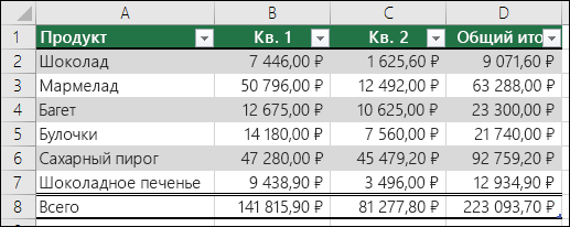
Чтобы упростить управление группой связанных данных и ее анализ, можно превратить диапазон ячеек в таблицу Excel (ранее Excel списком).
Элементы таблиц Microsoft Excel
Таблица может включать указанные ниже элементы.
-
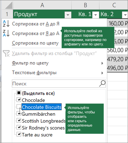
Строка заголовков. По умолчанию таблица включает строку заголовков. Для каждого столбца таблицы в строке заголовков включена возможность фильтрации, что позволяет быстро фильтровать или сортировать данные. Дополнительные сведения см. в сведениях Фильтрация данных и Сортировка данных.

Строку с заглавной строкой в таблице можно отключить. Дополнительные сведения см. в Excel или отключении Excel таблицы.
-
Чередование строк. Чередуясь или затеняя строками, можно лучше различать данные.
-
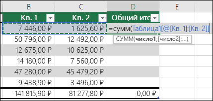
Вычисляемые столбцы. Введя формулу в одну ячейку столбца таблицы, можно создать вычисляемый столбец, ко всем остальным ячейкам которого будет сразу применена эта формула. Дополнительные сведения см. в статье Использование вычисляемой таблицы Excel столбцов.
-
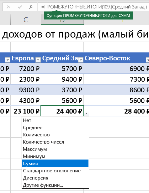
Строка итогов После добавления строки итогов в таблицу Excel вы можете выбрать один из таких функций, как СУММ, С СРЕДНЕЕ И так далее. При выборе одного из этих параметров таблица автоматически преобразует их в функцию SUBTOTAL, при этом будут игнорироваться строки, скрытые фильтром по умолчанию. Если вы хотите включить в вычисления скрытые строки, можно изменить аргументы функции SUBTOTAL.
Дополнительные сведения см. в этойExcel данных.
-
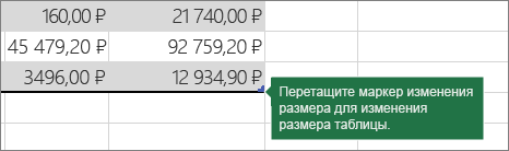
Маркер изменения размера. Маркер изменения размера в нижнем правом углу таблицы позволяет путем перетаскивания изменять размеры таблицы.
Другие способы переумноизации таблицы см. в статье Добавление строк и столбцов в таблицу с помощью функции «Избавься от нее».
Создание таблиц в базе данных
В таблице можно создать сколько угодно таблиц.
Чтобы быстро создать таблицу в Excel, сделайте следующее:
-
Вы выберите ячейку или диапазон данных.
-
На вкладке Главная выберите команду Форматировать как таблицу.
-
Выберите стиль таблицы.
-
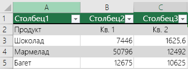
В диалоговом окне Форматировать как таблицу, если вы хотите, чтобы первая строка диапазона была строкой заглавных и нажмите кнопку ОК.
Также просмотрите видео о создании таблицы в Excel.
Эффективная работа с данными таблицы
Excel есть некоторые функции, которые позволяют эффективно работать с данными таблиц:
-
Использование структурированных ссылок. Вместо использования ссылок на ячейки, таких как A1 и R1C1, можно использовать структурированные ссылки, которые указывают на имена таблиц в формуле. Дополнительные сведения см. в теме Использование структурированных ссылок Excel таблиц.
-
Обеспечение целостности данных. Вы можете использовать встроенную функцию проверки данных в Excel. Например, можно разрешить ввод только чисел или дат в столбце таблицы. Дополнительные сведения о том, как обеспечить целостность данных, см. в теме Применение проверки данных к ячейкам.
Экспорт таблицы Excel на SharePoint
Если у вас есть доступ к SharePoint, вы можете экспортировать таблицу Excel в SharePoint список. Таким образом, другие люди смогут просматривать, редактировать и обновлять данные таблицы в SharePoint списке. Вы можете создать однонаправленную связь со списком SharePoint, чтобы на листе всегда учитывались изменения, вносимые в этот список. Дополнительные сведения см. в статье Экспорт таблицы Excel в SharePoint.
Дополнительные сведения
Вы всегда можете задать вопрос специалисту Excel Tech Community или попросить помощи в сообществе Answers community.
См. также
Форматирование таблицы Excel
Проблемы совместимости таблиц Excel
Нужна дополнительная помощь?
A spreadsheet is a computer application that is designed to add, display, analyze, organize, and manipulate data arranged in rows and columns. It is the most popular application for accounting, analytics, data presentation, etc. Or in other words, spreadsheets are scalable grid-based files that are used to organize data and perform calculations. People all across the world use spreadsheets to create tables for personal and business usage. You can also use the tool’s features and formulas to help you make sense of your data. You could, for example, track data in a spreadsheet and see sums, differences, multiplication, division, and fill dates automatically, among other things. Microsoft Excel, Google sheets, Apache open office, LibreOffice, etc are some spreadsheet software. Among all these software, Microsoft Excel is the most commonly used spreadsheet tool and it is available for Windows, macOS, Android, etc.
A collection of spreadsheets is known as a workbook. Every Excel file is called a workbook. Every time when you start a new project in Excel, you’ll need to create a new workbook. There are several methods for getting started with an Excel workbook. To create a new worksheet or access an existing one, you can either start from scratch or utilize a pre-designed template.
A single Excel worksheet is a tabular spreadsheet that consists of a matrix of rectangular cells grouped in rows and columns. It has a total of 1,048,576 rows and 16,384 columns, resulting in 17,179,869,184 cells on a single page of a Microsoft Excel spreadsheet where you may write, modify, and manage your data.
In the same way as a file or a book is made up of one or more worksheets that contain various types of related data, an Excel workbook is made up of one or more worksheets. You can also create and save an endless number of worksheets. The major purpose is to collect all relevant data in one place, but in many categories (worksheet).
Feature of spreadsheet
As we know that there are so many spreadsheet applications available in the market. So these applications provide the following basic features:
1. Rows and columns: Rows and columns are two distinct features in a spreadsheet that come together to make a cell, a range, or a table. In general, columns are the vertical portion of an excel worksheet, and there can be 256 of them in a worksheet, whereas rows are the horizontal portion, and there can be 1048576 of them.
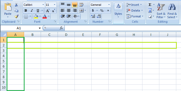
The color light green is used to highlight Row 3 while the color green is used to highlight Column B. Each column has 1048576 rows and each row has 256 columns.
2. Formulas: In spreadsheets, formulas process data automatically. It takes data from the specified area of the spreadsheet as input then processes that data, and then displays the output into the new area of the spreadsheet according to where the formula is written. In Excel, we can use formulas simply by typing “=Formula Name(Arguments)” to use predefined Excel formulas. When you write the first few characters of any formula, Excel displays a drop-down menu of formulas that match that character sequence. Some of the commonly used formulas are:
- =SUM(Arg1: Arg2): It is used to find the sum of all the numeric data specified in the given range of numbers.
- =COUNT(Arg1: Arg2): It is used to count all the number of cells(it will count only number) specified in the given range of numbers.
- =MAX(Arg1: Arg2): It is used to find the maximum number from the given range of numbers.
- =MIN(Arg1: Arg2): It is used to find the minimum number from the given range of numbers.
- =TODAY(): It is used to find today’s date.
- =SQRT(Arg1): It is used to find the square root of the specified cell.
For example, you can use the formula to find the average of the integers in column C from row 2 to row 7:
= AVERAGE(D2:D7)
The range of values on which you want to average is defined by D2:D6. The formula is located near the name field on the formula tab.
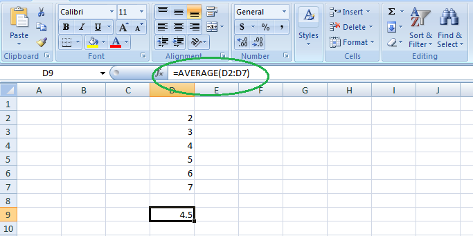
We wrote =AVERAGE(D2:D6) in cell D9, therefore the average becomes (2 + 3 + 4 + 5 + 6 + 7)/6 = 27/6 = 4.5. So you can quickly create a workbook, work on it, browse through it, and save it in this manner.
3. Function: In spreadsheets, the function uses a specified formula on the input and generates output. Or in other words, functions are created to perform complicated math problems in spreadsheets without using actual formulas. For example, you want to find the total of the numeric data present in the column then use the SUM function instead of adding all the values present in the column.
4. Text Manipulation: The spreadsheet provides various types of commands to manipulate the data present in it.
5. Pivot Tables: It is the most commonly used feature of the spreadsheet. Using this table users can organize, group, total, or sort data using the toolbar. Or in other words, pivot tables are used to summarize lots of data. It converts tons of data into a few rows and columns.
Use of Spreadsheets
The use of Spreadsheets is endless. It is generally used with anything that contains numbers. Some of the common use of spreadsheets are:
- Finance: Spreadsheets are used for financial data like it is used for checking account information, taxes, transaction, billing, budgets, etc.
- Forms: Spreadsheet is used to create form templates to manage performance review, timesheets, surveys, etc.
- School and colleges: Spreadsheets are most commonly used in schools and colleges to manage student’s data like their attendance, grades, etc.
- Lists: Spreadsheets are also used to create lists like grocery lists, to-do lists, contact detail, etc.
- Hotels: Spreadsheets are also used in hotels to manage the data of their customers like their personal information, room numbers, check-in date, check-out date, etc.
Components of Spreadsheets
The basic components of spreadsheets are:
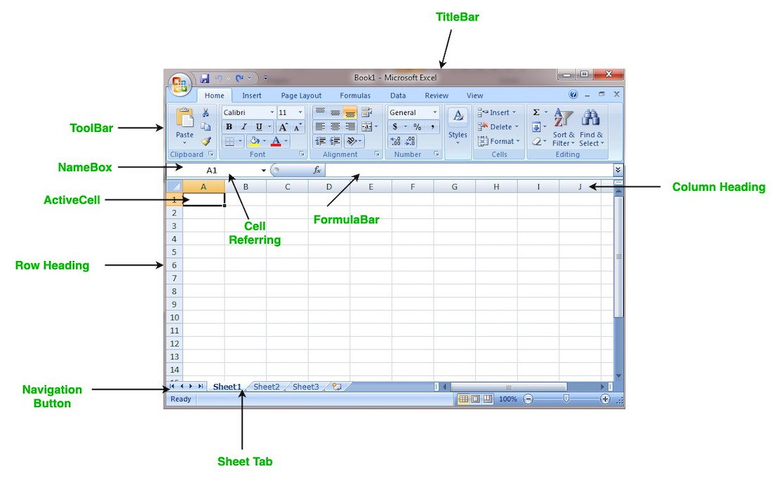
1. TitleBar: The title bar displays the name of the spreadsheet and application.
2. Toolbar: It displays all the options or commands available in Excel for use.
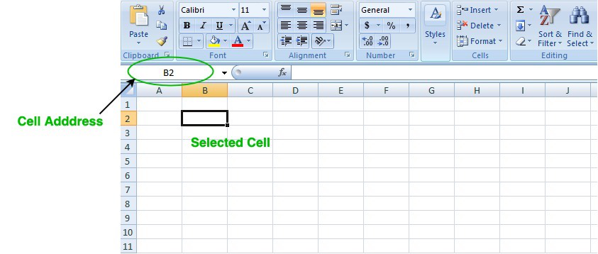
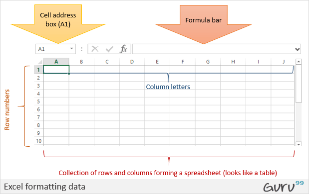
3. NameBox: It displays the address of the current or active cell.
4. Formula Bar: It is used to display the data entered by us in the active cell. Also, this bar is used to apply formulas to the data of the spreadsheet.
5. Column Headings: Every excel spreadsheet contains 256 columns and each column present in the spreadsheet is named by letters or a combination of letters.
6. Row Headings: Every excel spreadsheet contains 65,536 rows and each row present in the spreadsheet is named by a number.
7. Cell: In a spreadsheet, everything like a numeric value, functions, expressions, etc., is recorded in the cell. Or we can say that an intersection of rows and columns is known as a cell. Every cell has its own name or address according to its column and rows and when the cursor is present on the first cell then that cell is known as an active cell.
8. Cell referring: A cell reference, also known as a cell address, is a way for describing a cell on a worksheet that combines a column letter and a row number. We can refer to any cell on the worksheet using cell references (in excel formulae). As shown in the above image the cell in column A and row 1 is referred to as A1. Such notations can be used in any formula or to duplicate the value of one cell to another (by using = A1).
9. Navigation buttons: A spreadsheet contains first, previous, next, and last navigation buttons. These buttons are used to move from one worksheet to another workbook.
10. Sheet tabs: As we know that a workbook is a collection of worksheets. So this tab contains all the worksheets present in the workbook, by default it contains three worksheets but you can add more according to your requirement.
Create a new Spreadsheet or Workbook
To create a new spreadsheet follow the following steps:
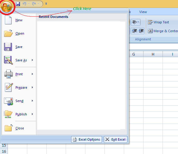
Step 1: Click on the top-left, Microsoft office button and a drop-down menu appear.
Step 2: Now select New from the menu.
Step 3: After selecting the New option a New Workbook dialogue box will appear and then in Create tab, click on the blank Document.
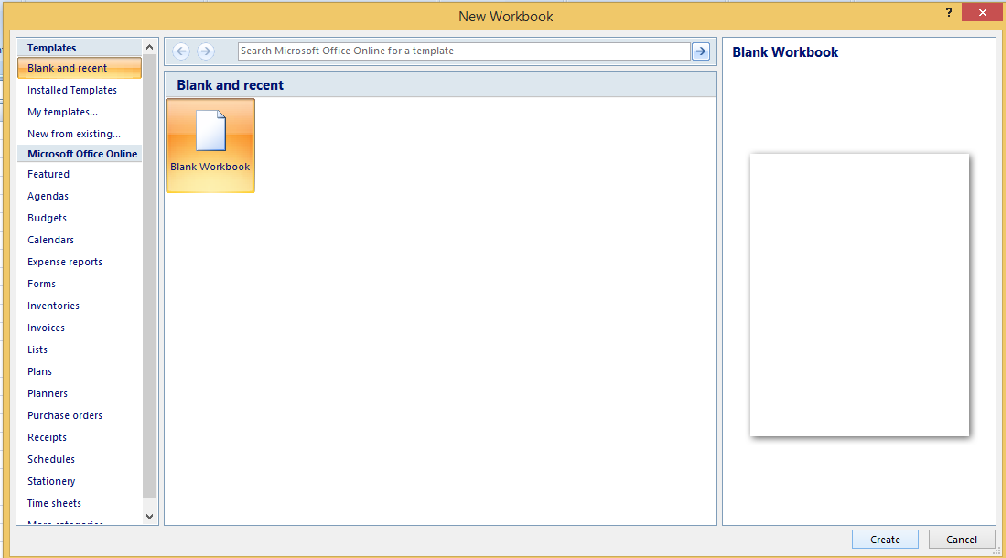
A new blank worksheet is created and is shown on your screen.
Note: When you open MS Excel on your computer, it creates a new Workbook for you.
Saving The Workbook
In Excel we can save a workbook using the following steps:
Step 1: Click on the top-left, Microsoft office button and we get a drop-down menu:
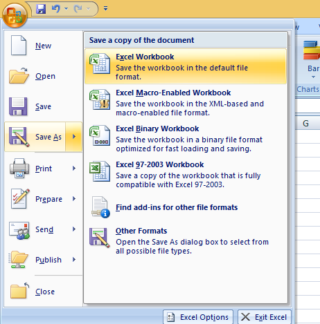
Step 2: Now Save or Save As are the options to save the workbook, so choose one.
- Save As: To name the spreadsheet and then save it to a specific location. Select Save As if you wish to save the file for the first time, or if you want to save it with a new name.
- Save: To save your work, select Save/ click ctrl + S if the file has already been named.
So this is how you can save a workbook in Excel.
Inserting text in Spreadsheet
Excel consists of many rows and columns, each rectangular box in a row or column is referred to as a Cell. So, the combination of a column letter and a row number can be used to find a cell address on a worksheet or spreadsheet. We can refer to any cell in the worksheet using these addresses (in excel formulas). The name box on the top left(below the Home tab) displays the cell’s address whenever you click the cell.
To insert the data into the cell follow the following steps:
Step 1: Go to a cell and click on it
Step 2: By typing something on the keyboard, you can insert your data (In that selected cell).
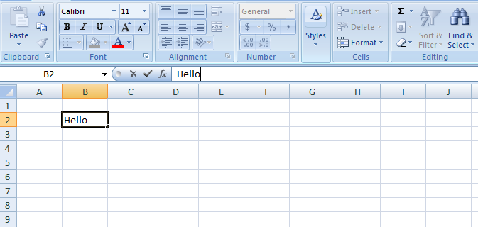
Whatever text you type displays in the formula bar as well (for that cell).
Edit/ Delete Cell Contents in the Spreadsheet
To delete cell content follow the following steps:
Step 1: To alter or delete the text in a cell, first select it.
Step 2: Press the Backspace key on your keyboard to delete and correct text. Alternatively, hit the Delete key to delete the whole contents of a cell. You can also edit and delete text using the formula bar. Simply select the cell and move the pointer to the formula bar.
Содержание
- What is Microsoft Excel and What Does It Do?
- What Excel Is Used For
- Spreadsheet Cells and Cell References
- Data Types, Formulas, and Functions
- Excel and Financial Data
- Excel’s Other Uses
- Excel Alternatives
- Introduction to Microsoft Excel 101: Notes About MS Excel
- What is Microsoft Excel?
- Why Should I Learn Microsoft Excel?
- Where can I get Microsoft Excel?
- How to Open Microsoft Excel?
- Understanding the Ribbon
- Ribbon components explained
- Understanding the worksheet (Rows and Columns, Sheets, Workbooks)
- Customization Microsoft Excel Environment
- Customization of ribbon
- Adding custom tabs to the ribbon
- Setting the colour theme
- Settings for formulas
- Proofing settings
- Save settings
What is Microsoft Excel and What Does It Do?
This versatile program helps you make sense of your data
:max_bytes(150000):strip_icc()/ryanperiansquare-de5f69cde760457facb17deac949263e-180a645bf10845498a859fbbcda36d46.jpg)
Excel is an electronic spreadsheet program that is used for storing, organizing, and manipulating data.
The information we’ve prepared refers to Microsoft Excel in general and is not limited to any specific version of the program.
What Excel Is Used For
Electronic spreadsheet programs were originally based on paper spreadsheets used for accounting. As such, the basic layout of computerized spreadsheets is the same as the paper ones. Related data is stored in tables — which are a collection of small rectangular boxes or cells organized into rows and columns.
All versions of Excel and other spreadsheet programs can store several spreadsheet pages in a single computer file. The saved computer file is often referred to as a workbook and each page in the workbook is a separate worksheet.
Spreadsheet Cells and Cell References
:max_bytes(150000):strip_icc()/RowsandColumns-5a690dd96edd650037ee83cd.jpg)
When you look at the Excel screen — or any other spreadsheet screen — you see a rectangular table or grid of rows and columns.
In newer versions of Excel, each worksheet contains roughly a million rows and more than 16,000 columns, which necessitates an addressing scheme in order to keep track of where data is located.
The horizontal rows are identified by numbers (1, 2, 3) and the vertical columns by letters of the alphabet (A, B, C). For columns beyond 26, columns are identified by two or more letters such as AA, AB, AC or AAA, AAB, etc.
The intersection point between a column and a row is the small rectangular box known as a cell. The cell is the basic unit for storing data in the worksheet, and because each worksheet contains millions of these cells, each one is identified by its cell reference.
A cell reference is a combination of the column letter and the row number such as A3, B6, and AA345. In these cell references, the column letter is always listed first.
Data Types, Formulas, and Functions
:max_bytes(150000):strip_icc()/Formula-5a690e6d1f4e130039a7d806.jpg)
The types of data that a cell can hold include:
- Numbers
- Text
- Dates and times
- Boolean values
- Formulas
Formulas are used for calculations — usually incorporating data contained in other cells. These cells, however, may be located on different worksheets or in different workbooks.
Creating a formula starts by entering the equal sign in the cell where you want the answer displayed. Formulas can also include cell references to the location of data and one or more spreadsheet functions.
Functions in Excel and other electronic spreadsheets are built-in formulas that are designed to simplify carrying out a wide range of calculations – from common operations such as entering the date or time to more complex ones such as finding specific information located in large tables of data.
Excel and Financial Data
:max_bytes(150000):strip_icc()/FinancialData-5a690eff3de423001a6bea13.jpg)
Spreadsheets are often used to store financial data. Formulas and functions that are used on this type of data include:
- Performing basic mathematical operations such as summing columns or rows of numbers
- Finding values such as profit or loss
- Calculating repayment plans for loans or mortgages
- Finding the average, maximum, minimum and other statistical values in a specified range of data
- Carrying out What-If analysis on data, where variables are modified one at a time to see how the change affects other data, such as expenses and profits
Excel’s Other Uses
:max_bytes(150000):strip_icc()/Charttools-5a690f77c673350019bb304b.jpg)
Other common operations that Excel can be used for include:
- Graphing or charting data to assist users in identifying data trends
- Formatting data to make important data easy to find and understand
- Printing data and charts for use in reports
- Sorting and filtering data to find specific information
- Linking worksheet data and charts for use in other programs such as Microsoft PowerPoint and Word
- Importing data from database programs for analysis
Spreadsheets were the original «killer apps» for personal computers because of their ability to compile and make sense of information. Early spreadsheet programs such as VisiCalc and Lotus 1-2-3 were largely responsible for the growth in popularity of computers like the Apple II and the IBM PC as a business tool.
Excel Alternatives
:max_bytes(150000):strip_icc()/TCSQ1-5a690c6b3418c6001912517e.jpg)
Other current spreadsheet programs that are available for use include:
- Google Sheets: A free, web-based spreadsheet program
- Excel Online: A free, scaled-down, web-based version of Excel
- Open Office Calc: A free, downloadable spreadsheet program.
Get the Latest Tech News Delivered Every Day
Источник
Introduction to Microsoft Excel 101: Notes About MS Excel
Updated February 25, 2023
What is Microsoft Excel?
Microsoft Excel is a spreadsheet program used to record and analyze numerical and statistical data. Microsoft Excel provides multiple features to perform various operations like calculations, pivot tables, graph tools, macro programming, etc. It is compatible with multiple OS like Windows, macOS, Android and iOS.
A Excel spreadsheet can be understood as a collection of columns and rows that form a table. Alphabetical letters are usually assigned to columns, and numbers are usually assigned to rows. The point where a column and a row meet is called a cell. The address of a cell is given by the letter representing the column and the number representing a row.
Why Should I Learn Microsoft Excel?
We all deal with numbers in one way or the other. We all have daily expenses which we pay for from the monthly income that we earn. For one to spend wisely, they will need to know their income vs. expenditure. Microsoft Excel comes in handy when we want to record, analyze and store such numeric data. Let’s illustrate this using the following image.
Where can I get Microsoft Excel?
There are number of ways in which you can get Microsoft Excel. You can buy it from a hardware computer shop that also sells software. Microsoft Excel is part of the Microsoft Office suite of programs. Alternatively, you can download it from the Microsoft website but you will have to buy the license key.
In this Microsoft Excel tutorial, we are going to cover the following topics about MS Excel.
How to Open Microsoft Excel?
Running Excel is not different from running any other Windows program. If you are running Windows with a GUI like (Windows XP, Vista, and 7) follow the following steps.
- Click on start menu
- Point to all programs
- Point to Microsoft Excel
- Click on Microsoft Excel
Alternatively, you can also open it from the start menu if it has been added there. You can also open it from the desktop shortcut if you have created one.
For this tutorial, we will be working with Windows 8.1 and Microsoft Excel 2013. Follow the following steps to run Excel on Windows 8.1
- Click on start menu
- Search for Excel N.B. even before you even typing, all programs starting with what you have typed will be listed.
- Click on Microsoft Excel
The following image shows you how to do this
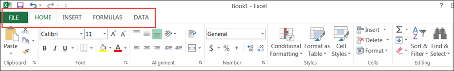
Understanding the Ribbon
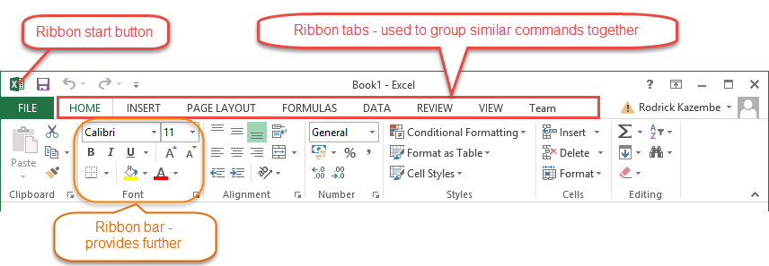
The ribbon provides shortcuts to commands in Excel. A command is an action that the user performs. An example of a command is creating a new document, printing a documenting, etc. The image below shows the ribbon used in Excel 2013.
Ribbon components explained
Ribbon start button – it is used to access commands i.e. creating new documents, saving existing work, printing, accessing the options for customizing Excel, etc.
Ribbon tabs – the tabs are used to group similar commands together. The home tab is used for basic commands such as formatting the data to make it more presentable, sorting and finding specific data within the spreadsheet.
Ribbon bar – the bars are used to group similar commands together. As an example, the Alignment ribbon bar is used to group all the commands that are used to align data together.
Understanding the worksheet (Rows and Columns, Sheets, Workbooks)
A worksheet is a collection of rows and columns. When a row and a column meet, they form a cell. Cells are used to record data. Each cell is uniquely identified using a cell address. Columns are usually labelled with letters while rows are usually numbers.
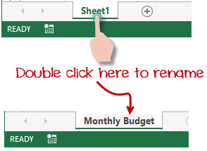
A workbook is a collection of worksheets. By default, a workbook has three cells in Excel. You can delete or add more sheets to suit your requirements. By default, the sheets are named Sheet1, Sheet2 and so on and so forth. You can rename the sheet names to more meaningful names i.e. Daily Expenses, Monthly Budget, etc.
Customization Microsoft Excel Environment
Personally I like the black colour, so my excel theme looks blackish. Your favourite colour could be blue, and you too can make your theme colour look blue-like. If you are not a programmer, you may not want to include ribbon tabs i.e. developer. All this is made possible via customizations. In this sub-section, we are going to look at;
- Customization the ribbon
- Setting the colour theme
- Settings for formulas
- Proofing settings
- Save settings
Customization of ribbon
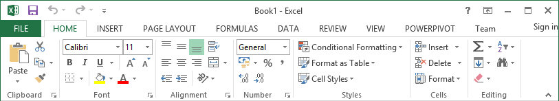
The above image shows the default ribbon in Excel 2013. Let’s start with customization the ribbon, suppose you do not wish to see some of the tabs on the ribbon, or you would like to add some tabs that are missing such as the developer tab. You can use the options window to achieve this.
- Click on the ribbon start button
- Select options from the drop down menu. You should be able to see an Excel Options dialog window
- Select the customize ribbon option from the left-hand side panel as shown below
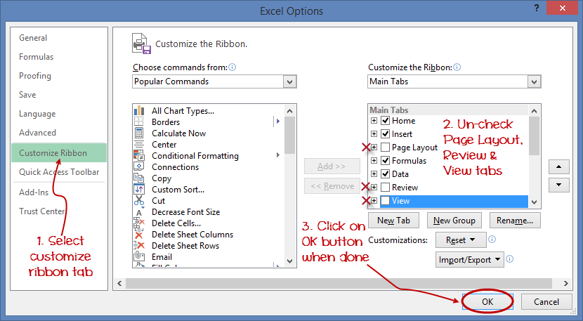
- On your right-hand side, remove the check marks from the tabs that you do not wish to see on the ribbon. For this example, we have removed Page Layout, Review, and View tab.
- Click on the “OK” button when you are done.
Your ribbon will look as follows
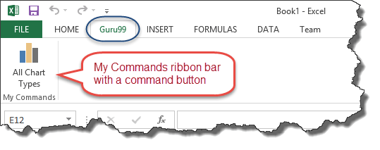
Adding custom tabs to the ribbon
You can also add your own tab, give it a custom name and assign commands to it. Let’s add a tab to the ribbon with the text Guru99

- Right click on the ribbon and select Customize the Ribbon. The dialogue window shown above will appear
- Click on new tab button as illustrated in the animated image below
- Select the newly created tab
- Click on Rename button
- Give it a name of Guru99
- Select the New Group (Custom) under Guru99 tab as shown in the image below
- Click on Rename button and give it a name of My Commands
- Let’s now add commands to my ribbon bar
- The commands are listed on the middle panel
- Select All chart types command and click on Add button
- Click on OK
Your ribbon will look as follows
Setting the colour theme
To set the color-theme for your Excel sheet you have to go to Excel ribbon, and click on à File àOption command. It will open a window where you have to follow the following steps.
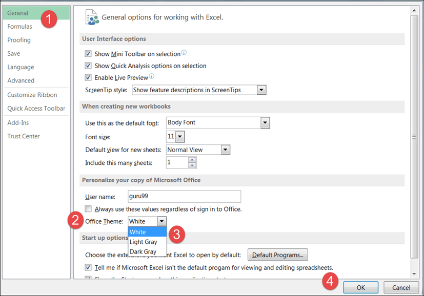
- The general tab on the left-hand panel will be selected by default.
- Look for colour scheme under General options for working with Excel
- Click on the colour scheme drop-down list and select the desired colour
- Click on OK button
Settings for formulas
This option allows you to define how Excel behaves when you are working with formulas. You can use it to set options i.e. autocomplete when entering formulas, change the cell referencing style and use numbers for both columns and rows and other options.
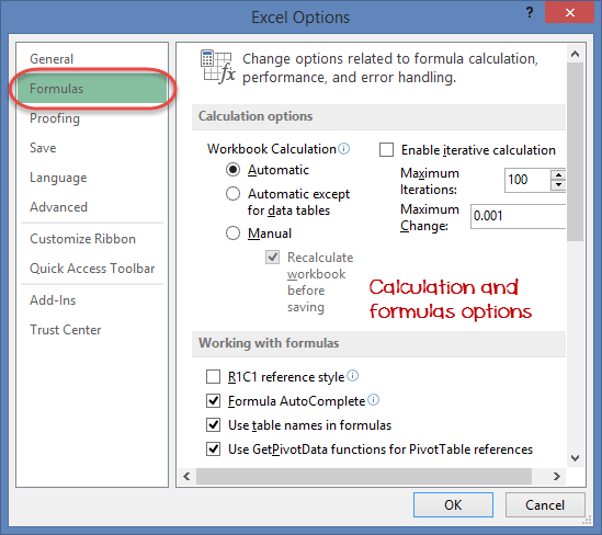
If you want to activate an option, click on its check box. If you want to deactivate an option, remove the mark from the checkbox. You can this option from the Options dialogue window under formulas tab from the left-hand side panel
Proofing settings
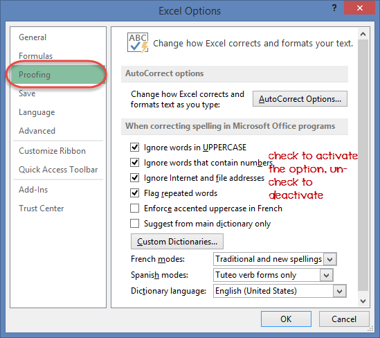
This option manipulates the entered text entered into excel. It allows setting options such as the dictionary language that should be used when checking for wrong spellings, suggestions from the dictionary, etc. You can this option from the options dialogue window under the proofing tab from the left-hand side panel
Save settings
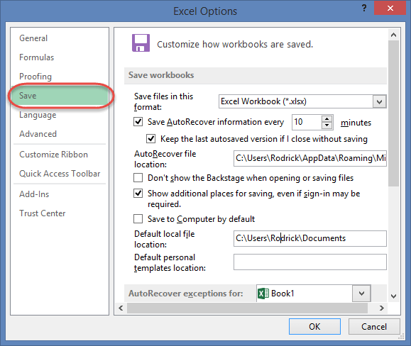
This option allows you to define the default file format when saving files, enable auto recovery in case your computer goes off before you could save your work, etc. You can use this option from the Options dialogue window under save tab from the left-hand side panel
Источник
Every modern PC user, at least oncefaced with a package of programs Microsoft Office, which is now one of the most common, knows that it necessarily contains an application MS Excel. Now we will consider the basic concept of spreadsheets. In passing, brief information about the main elements of the structure of table elements and data and some of their possibilities will be given.
What is an Excel spreadsheet?
The first mention of the Excel program dates back to 1987, when Microsoft released its most famous office suite of applications and programs, united by the common name MS Office.

In fact, the Excel spreadsheet representsa universal means of processing mathematical data of all varieties and levels of complexity. This includes mathematics, algebra, geometry, trigonometry, working with matrices, mathematical analysis, solving complex systems of equations, and much more. Practically everything that belongs to the exact sciences of this plan is presented in the program itself. The functions of spreadsheets are such that many users not only do not know about them, they do not even suspect how powerful this software product is. But first things first.
Getting Started with Spreadsheets
Once the user opens the programExcel, he sees in front of him a table created from the so-called default template. The main working area consists of columns and rows, the intersection of which forms cells. In the understanding of working with all types of data, the main element of the spreadsheet is a cell, because it is in it that they are entered.

Each cell has a numbering consisting ofordinal designation of a column and a row, however, it may differ in different versions of the application. For example, in the 2003 version, the very first cell located at the intersection of column «A» and line «1» is designated as «A1». In the 2010 version, this approach was changed. Here the designation is represented as serial numbers and numbers, but in the description line the columns are designated as «C», and the lines as «R». Many people do not understand why this is so. But here everything is simple: «R» is the first letter of the English word row (row, row), and «C» is the first letter of the word column (column).
Used data
Speaking about the fact that the main element of the electronicThe table is a cell, you need to understand that it concerns exclusively input data (values, text, formulas, functional dependencies, etc.). The data in the cells can have a different format. The function of changing the format of the cell can be called from the context menu when the PCM is clicked on (right-click).

Data can be presented in text,numeric, percentage, exponential, monetary (currency), fractional and time formats, as well as in the form of a date. In addition, you can specify additional parameters for a kind or decimal places when using numbers.
Main window of the program: structure
If you look closely at the main windowyou can see that in the standard version, the table can contain 256 columns and 65536 rows. The bottom of the tabs are tabs. There are three of them in the new file, but you can ask more. If you consider that the main element of the spreadsheet is a sheet, this concept must be attributed to the content on different sheets of different data that can be used crosswise when specifying the appropriate formulas and functions.

Such operations are most applicable when creatingsummary tables, reports or complex computation systems. Separately, it should be said that if there are interlinked data on different sheets, the result is automatically calculated without changing the dependent cells and sheets without reintroducing a formula or function expressing this or that dependence of the variables and constants.
On top is a standard panel withseveral main menus, and just below the formula line. Speaking about the data contained in the cells, we can say that the main element of the spreadsheet is this element, because the line itself displays either text or numeric data entered into cells, or the formulas and functional dependencies. In the sense of displaying information, the formula string and the cell are the same. True, for a string, formatting or specifying a data type is not applicable. This is exclusively a viewer and input.
Formulas in Excel spreadsheets
As for the formulas, they are sufficient in the programa lot of. Some of them are unknown to many users in general. Of course, to understand all of them, you can carefully read the same reference manual, but the program also provides a special opportunity for automation of the process.

When you click on the button «fx«(Or the sign»=«) A list will be displayed, from which you can select the necessary action, which will save the user from manually entering the formula.

There is one more frequently used remedy. This is an auto-sum function, represented as a button on the toolbar. Here, too, the formula will not be introduced. It is enough to activate the cell in the row and column after the selected range, where it is supposed to be calculated, and click on the button. And this is not the only example.
Interconnected data, sheets, files and cross-references
With regard to interlinked links,the cell and the sheet can be attached data from another location in this document, a third-party file, data from some Internet resource, or an executable script. This allows you to even save disk space and reduce the original size of the document itself. Naturally, how to create such interrelations, it is necessary to understand carefully. But, as they say, there would be a desire.
Add-ins, diagrams and graphs
In terms of additional tools andMS Excel spreadsheets provide the user with a wide choice. Not to mention the specific add-ons or executable Java or Visual Basic scripts, let’s dwell on creating graphical visual tools for viewing the analysis results.
It is clear that drawing a diagram or buildinga graph based on a huge amount of dependent data manually, and then inserting such a graphic object into a table as a separate file or an attached image is not something everyone wants.

That is why their automaticcreation with a preliminary choice of type and type. It is clear that they are based on a certain data area. Just in the construction of graphs and diagrams, it can be argued that the main element of the spreadsheet is a selected area or several areas on different sheets or in different attached files, from which the values of variables and dependent computational results will be taken.
Applying filters
In some cases, it may be necessaryThe use of special filters that are installed on one or more columns. In the simplest form, it helps to search for data, text or values in the entire column. On coincidence, all the results found will be shown separately.

If there are dependencies, together withthe filtered data of one column will show the remaining values located in the other columns and rows. But this is the simplest example, because each user filter has its own submenu with certain search criteria or a specific setting.
Conclusion
Of course, consider in one article allthe possibilities of MS Excel are simply impossible. At least here you can understand what elements are the main ones in the tables, based on each specific case or situation, and also at least a little understanding, so to speak, with the basics of work in this unique program. But to fully master it will have to work hard. Often, and the developers themselves do not always know what their offspring are capable of.
</ p>>
In this Microsoft Excel tutorial, we will learn the Microsoft Exel basics. These Microsoft Excel notes will help you learn every MS Excel concepts. Let’s start with the introduction:
What is Microsoft Excel?
Microsoft Excel is a spreadsheet program used to record and analyze numerical and statistical data. Microsoft Excel provides multiple features to perform various operations like calculations, pivot tables, graph tools, macro programming, etc. It is compatible with multiple OS like Windows, macOS, Android and iOS.
A Excel spreadsheet can be understood as a collection of columns and rows that form a table. Alphabetical letters are usually assigned to columns, and numbers are usually assigned to rows. The point where a column and a row meet is called a cell. The address of a cell is given by the letter representing the column and the number representing a row.
Why Should I Learn Microsoft Excel?
We all deal with numbers in one way or the other. We all have daily expenses which we pay for from the monthly income that we earn. For one to spend wisely, they will need to know their income vs. expenditure. Microsoft Excel comes in handy when we want to record, analyze and store such numeric data. Let’s illustrate this using the following image.
Where can I get Microsoft Excel?
There are number of ways in which you can get Microsoft Excel. You can buy it from a hardware computer shop that also sells software. Microsoft Excel is part of the Microsoft Office suite of programs. Alternatively, you can download it from the Microsoft website but you will have to buy the license key.
In this Microsoft Excel tutorial, we are going to cover the following topics about MS Excel.
- How to Open Microsoft Excel?
- Understanding the Ribbon
- Understanding the worksheet
- Customization Microsoft Excel Environment
- Important Excel shortcuts
How to Open Microsoft Excel?
Running Excel is not different from running any other Windows program. If you are running Windows with a GUI like (Windows XP, Vista, and 7) follow the following steps.
- Click on start menu
- Point to all programs
- Point to Microsoft Excel
- Click on Microsoft Excel
Alternatively, you can also open it from the start menu if it has been added there. You can also open it from the desktop shortcut if you have created one.
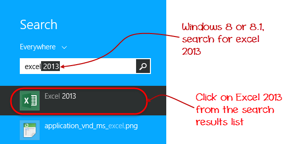
For this tutorial, we will be working with Windows 8.1 and Microsoft Excel 2013. Follow the following steps to run Excel on Windows 8.1
- Click on start menu
- Search for Excel N.B. even before you even typing, all programs starting with what you have typed will be listed.
- Click on Microsoft Excel
The following image shows you how to do this
Understanding the Ribbon
The ribbon provides shortcuts to commands in Excel. A command is an action that the user performs. An example of a command is creating a new document, printing a documenting, etc. The image below shows the ribbon used in Excel 2013.
Ribbon components explained
Ribbon start button – it is used to access commands i.e. creating new documents, saving existing work, printing, accessing the options for customizing Excel, etc.
Ribbon tabs – the tabs are used to group similar commands together. The home tab is used for basic commands such as formatting the data to make it more presentable, sorting and finding specific data within the spreadsheet.
Ribbon bar – the bars are used to group similar commands together. As an example, the Alignment ribbon bar is used to group all the commands that are used to align data together.
Understanding the worksheet (Rows and Columns, Sheets, Workbooks)
A worksheet is a collection of rows and columns. When a row and a column meet, they form a cell. Cells are used to record data. Each cell is uniquely identified using a cell address. Columns are usually labelled with letters while rows are usually numbers.
A workbook is a collection of worksheets. By default, a workbook has three cells in Excel. You can delete or add more sheets to suit your requirements. By default, the sheets are named Sheet1, Sheet2 and so on and so forth. You can rename the sheet names to more meaningful names i.e. Daily Expenses, Monthly Budget, etc.
Customization Microsoft Excel Environment
Personally I like the black colour, so my excel theme looks blackish. Your favourite colour could be blue, and you too can make your theme colour look blue-like. If you are not a programmer, you may not want to include ribbon tabs i.e. developer. All this is made possible via customizations. In this sub-section, we are going to look at;
- Customization the ribbon
- Setting the colour theme
- Settings for formulas
- Proofing settings
- Save settings
Customization of ribbon
The above image shows the default ribbon in Excel 2013. Let’s start with customization the ribbon, suppose you do not wish to see some of the tabs on the ribbon, or you would like to add some tabs that are missing such as the developer tab. You can use the options window to achieve this.
- Click on the ribbon start button
- Select options from the drop down menu. You should be able to see an Excel Options dialog window
- Select the customize ribbon option from the left-hand side panel as shown below
- On your right-hand side, remove the check marks from the tabs that you do not wish to see on the ribbon. For this example, we have removed Page Layout, Review, and View tab.
- Click on the “OK” button when you are done.
Your ribbon will look as follows
Adding custom tabs to the ribbon
You can also add your own tab, give it a custom name and assign commands to it. Let’s add a tab to the ribbon with the text Guru99
- Right click on the ribbon and select Customize the Ribbon. The dialogue window shown above will appear
- Click on new tab button as illustrated in the animated image below
- Select the newly created tab
- Click on Rename button
- Give it a name of Guru99
- Select the New Group (Custom) under Guru99 tab as shown in the image below
- Click on Rename button and give it a name of My Commands
- Let’s now add commands to my ribbon bar
- The commands are listed on the middle panel
- Select All chart types command and click on Add button
- Click on OK
Your ribbon will look as follows
Setting the colour theme
To set the color-theme for your Excel sheet you have to go to Excel ribbon, and click on à File àOption command. It will open a window where you have to follow the following steps.
- The general tab on the left-hand panel will be selected by default.
- Look for colour scheme under General options for working with Excel
- Click on the colour scheme drop-down list and select the desired colour
- Click on OK button
Settings for formulas
This option allows you to define how Excel behaves when you are working with formulas. You can use it to set options i.e. autocomplete when entering formulas, change the cell referencing style and use numbers for both columns and rows and other options.
If you want to activate an option, click on its check box. If you want to deactivate an option, remove the mark from the checkbox. You can this option from the Options dialogue window under formulas tab from the left-hand side panel
Proofing settings
This option manipulates the entered text entered into excel. It allows setting options such as the dictionary language that should be used when checking for wrong spellings, suggestions from the dictionary, etc. You can this option from the options dialogue window under the proofing tab from the left-hand side panel
Save settings
This option allows you to define the default file format when saving files, enable auto recovery in case your computer goes off before you could save your work, etc. You can use this option from the Options dialogue window under save tab from the left-hand side panel
Important Excel shortcuts
| Ctrl + P | used to open the print dialogue window |
| Ctrl + N | creates a new workbook |
| Ctrl + S | saves the current workbook |
| Ctrl + C | copy contents of current select |
| Ctrl + V | paste data from the clipboard |
| SHIFT + F3 | displays the function insert dialog window |
| SHIFT + F11 | Creates a new worksheet |
| F2 | Check formula and cell range covered |
Best Practices when working with Microsoft Excel
- Save workbooks with backward compatibility in mind. If you are not using the latest features in higher versions of Excel, you should save your files in 2003 *.xls format for backwards compatibility
- Use description names for columns and worksheets in a workbook
- Avoid working with complex formulas with many variables. Try to break them down into small managed results that you can use to build on
- Use built-in functions whenever you can instead of writing your own formulas
Summary
- Introduction of MS Excel : Microsoft Excel is a powerful spreadsheet program used to record, manipulate, store numeric data and it can be customized to match your preferences
- The ribbon is used to access various commands in Excel
- The options dialogue window allows you to customize a number of items i.e. the ribbon, formulas, proofing, save, etc.