Fuzzy match for excel

Одна из самых неприятных ситуаций, с которой может столкнуться пользователь при работе в Microsoft Excel — это поиск и подстановка данных с неточным совпадением. Когда вам надо подставить данные из одной таблицы в другую, но вы при этом уверены, что в обеих таблицах совпадающие элементы называются одинаково, то проблем нет — к вашим услугам множество способов: функции ВПР и её аналоги, надстройка Power Query и т.д.

А вот если в одной таблице «Пупкин Василий», а в другой просто «Пупкин», или «Пупкин В.», или даже «Пупкен», то все эти красивые способы не работают. Причем на практике такое встречается постоянно, особенно с почтовыми адресами или названиями компаний:

Обратите внимание на различные типы несоответствий, которые могут встречаться:

• переставлены местами улица, город, дом
• отсутствует какая-то часть адреса или, наоборот, есть что-то лишнее (индекс, номер квартиры)
• по-разному записан город (с буквой «г.» или без) или улица
• опечатки и ошибки (Козань вместо Казань)

Про точное соответствие или даже поиск по маске тут говорить не приходится. Помочь в таком случае могут только специальные макросы или надстройки для Excel. Про одну из таких макро-функций на VBA я уже писал, а здесь хочется рассказать про еще один вариант решения подобной задачи — надстройку Fuzzy Lookup от компании Microsoft.

Эта надстройка существует с 2011 года и совершенно бесплатно скачивается с сайта Microsoft. Системные требования: Windows 7 или новее, Office 2007 или новее, соответственно. После установки у вас в Excel появляется одноименная вкладка с единственной кнопкой на ней:

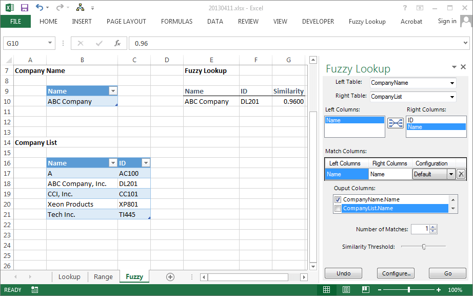
Нажатие на эту кнопку включает специальную панель в правой части окна Excel, где и задаются все настройки поиска:

Сразу хочу отметить, что эта надстройка умеет работать только с умными таблицами, поэтому все исходные таблицы нужно конвертировать в умные с помощью сочетания Ctrl+T или кнопки Форматировать как таблицу на вкладке Главная (Home — Format as Table):

Алгоритм действий при работе с надстройкой Fuzzy Lookup следующий:

1. Выберите какие таблицы нужно связать в выпадающих списках Left и Right Table.
2. Выберите ключевые столбцы в левой и правой таблицах, по которым нужно проверить соответствие и нажмите кнопку для добавления созданной пары в список Match Columns
3. В списке Output Columns отметьте галочками столбцы, которые вы хотите получить на выходе в качестве результата.
4. Установите активную ячейку в пустое место на листе, куда вы хотите вывести данные
5. Нажмите кнопку Go

После анализа мы получаем таблицу, где каждому элементу ключевого столбца из первой таблицы подобрано максимально похожее значение из второй:

Лепота!

Нюансы и подводные камни

• Точность подбора можно регулировать с помощью ползунка Similarity Threshold в нижней части панели Fuzzy Lookup. Чем правее его положение, тем строже будет поиск, и — как следствие — тем меньше результатов надстройка будет находить. Если сдвинуть его влево, то результатов станет больше, но возрастет риск ошибочного совпадения. Тут все зависит от вашей конкретной ситуации — экспериментируйте.
• На больших таблицах поиск может занимать приличное количество времени (до нескольких десятков секунд), хотя многое, конечно, зависит от мощности вашего компьютера. Как вариант, для ускорения в настройках (кнопка Configure в нижней части панели) можно попробовать включить параметр UseApproximateIndexing в разделе Global Settings.
• Перед нажатием на кнопку Go не забудьте выделить пустую ячейку, начиная с которой вы хотите вывести результаты. Если случайно вы оставите активную ячейку где-нибудь в исходных данных, то надстройка выведет итоговую таблицу прямо поверх них, и вы их потеряете. Причем отмена последнего действия будет невозможна, а кнопка Undo в нижней части панели не всегда срабатывает почему-то.
• Для вывода столбца с коэффициентом подобия FuzzyLookup.Similarity необходимо, чтобы у вашего Excel была точка в качестве десятичного разделителя (целой и дробной части). Если это не так, то эту настройку временно можно поменять через Файл — Параметры — Дополнительно (File — Options — Advanced).
• Fuzzy Lookup — это не обычная надстройка, написанная на VBA (как мой PLEX, например), а COM-надстройка. Разница в том, что она устанавливается как отдельная программа, т.е. вам нужны соответствующие права на установку ПО на вашем компьютере. Дома, ясное дело, проблем не будет, а вот многим корпоративным пользователям, скорее всего, придется обращаться к вашим айтишникам. После установки отключать и подключать ее в дальнейшем можно на вкладке Разработчик — Надстройки COM (Developer — COM Add-ins).

В любом случае, при всех имеющихся минусах, эта надстройка однозначно стоит того, чтобы находиться в арсенале любого продвинутого пользователя Microsoft Excel.

Ссылки по теме

This post explores Excel’s lookup functions, approximate matches, fuzzy lookups, and exact matches.  The built-in Excel lookup functions, such as VLOOKUP, are amazing. When implemented in the right way for special projects or in recurring use workbooks, they are able to save a ton of time. The VLOOKUP function alone has saved countless hours in my recurring use workbooks. However, the VLOOKUP function, similar to Excel’s other lookup functions such as HLOOKUP and MATCH, is built to perform an exact match or a range lookup. Both of these are quite different from an approximate match or a fuzzy lookup. This post discusses the details of these ideas, and demonstrates how to perform a fuzzy lookup in Excel 2010 and later.

*** UPDATED BLOG POST: FUZZY MATCH IS AVAILABLE IN POWER QUERY ***

Understanding Built-In Lookup Functions

The built-in Excel lookup functions, such as VLOOKUP, HLOOKUP, and MATCH, work with similar lookup logic.  To simplify this post, we’ll use just one as the example.  Since the VLOOKUP function is probably the most used and most familiar lookup function, we’ll use it as we explore these ideas.

The basic idea of an Excel lookup function is to look for a value in a list.  For example, we could ask Excel to find “ABC Company” in a list of customer names.  That is the basic idea, but the application of lookup functions are numerous and the implementations can become quite sophisticated and powerful.

For this post, I’d like to split the tasks that a lookup function performs into two steps.  I’ll call step one the match, and step two the return. In the first step, the match, Excel must find the matching value.  You tell Excel the value to find, such as “ABC Company” and you tell Excel where to look, such as in a range of cells.  You are asking Excel to find the lookup value in the lookup range.

Step two, the return, is the function’s result. That is, what value the function should return to the cell.  Some lookup functions, such as the MATCH function, tell Excel to return the position number.  Other lookup functions, such as the VLOOKUP function, tell Excel to return a related value.  So, based on which lookup function you select, and which function argument values you enter, Excel knows what to return once it finds its match. So far so good?

Let’s do a quick example at this point.

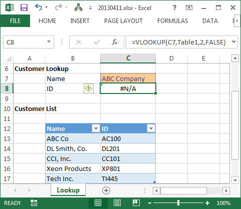
I would like to find a specific customer name “ABC Company” in a list of customers, and if found, I would like Excel to return the customer id which is found in the next column.

I would use a VLOOKUP function, and I would ask it to find “ABC Company” in the Customer Table, and return the ID.  Assuming the customer name was entered in C7, and the customers were stored in a Table named Table1, then the following function would do the trick:

=VLOOKUP(C7, Table1, 2, FALSE)

Where:

• C7 is the value to find
• Table1 is the lookup range
• 2 is the column that has the value we wish to return
• FALSE means we are not performing a range lookup

This function is entered in C8 in the screenshot below.

As you can see, the ID AC100 was successfully returned to the formula cell C8.  And that my friend is the basic idea of the VLOOKUP function.  Find a value (the match) and compute the result (the return).

It is important to note that the lookup value, the text string “ABC Company” must be found in the lookup range.  Except for case (upper and lower), the two values must match exactly.  “ABC Company” would not match “ABC Company, Inc.”, “ABC Co”, or “ABC Company   “.  No leading spaces, no trailing spaces, no extra abbreviations or characters.  They must be the same.  This is called an exact match.  If the value is not the same, the function will not match it, and you’ll get an error, as shown in the screenshot below.

Now that we have covered the basics, it is time to explore the VLOOKUP’s fourth argument.

 The Truth about the VLOOKUP Fourth Argument

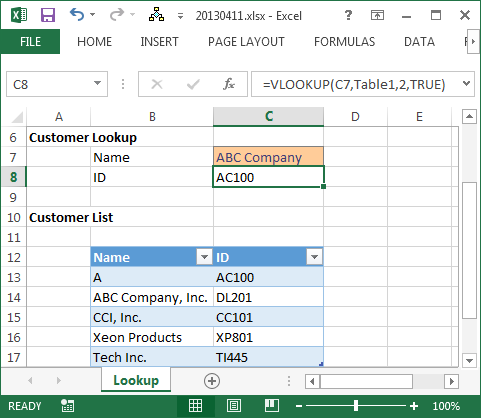
The fourth argument of the VLOOKUP function is officially named: range_lookup.  It is a boolean argument, meaning you can pass it a value of TRUE or FALSE, or any other representation of TRUE or FALSE. The thing that tends to mislead Excel users is the description that Microsoft used for these options.  Excel describes the TRUE value as “Approximate Match” and FALSE as “Exact Match.” A clearer description would have been something like TRUE “You are doing a range lookup” and FALSE “You are not doing a range lookup” but in any event, the descriptions are what they are.

When you select TRUE (Approximate Match) you are not asking Excel to match values that are approximately the same as each other.  The description Approximate Match would tend to imply that the function would match “ABC Company” and “ABC Company, Inc.” since they are approximately the same name.  In some cases and in some data sets, this idea would work.  But this idea does not work in all cases, and thus, can’t be relied upon in our workbooks.  For example, in the screenshot below, the function did not find a match between “ABC Company” and “ABC Company, Inc.” as evidenced by the incorrect ID returned in C8:

In the following screenshot however, the function did find a match between “ABC Company” and “ABC Co” as evidenced by the expected ID returned to C8:

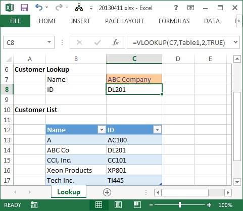
The way that the function actually works when TRUE is selected is this: it walks down the list row by row, and ultimately stops on the row that is less than the value and where the next row is greater than the value.  This is why the lookup range must be sorted in ascending order for the function to return an accurate result when the fourth argument is TRUE.

This idea can be confusing when thinking about text strings, but makes more sense when thinking about numbers.  For example, when trying to find the correct commission rate based on the sales value.  In this case, you want to perform a range lookup.  You want to look up a value from within a range.  This is illustrated in the screenshot below.

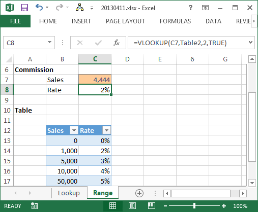
The function walks down row by row trying to determine which row to stop on.  It continues down until it finds a row that is greater than the lookup value, and then it stops on the previous row.  It stops on the row that is less than the value, and where the next row is greater than the lookup value.  This is pretty easy to understand when thinking about numbers, but can be harder to visualize when thinking about text strings. The key to understanding this function argument however, is to realize that the logic is identical when operating on text strings and numbers.  This is why “ABC Company” does not match “ABC Company, Inc.”, because “ABC Company Inc.” is greater than ABC Company.  This is why “ABC Company” will match “ABC Co”, because “ABC Co” is less than “ABC Company.”  As you can see, this is not what we have in mind when thinking about approximate match.

What is a Fuzzy Lookup aka Approximate Match

An approximate match, to us, means that two text strings that are about the same, but not necessarily identical, should match.  For example, “ABC Company” should match “ABC Company, Inc.,” “ABC Co,” and “ABC Company   .”  We think about an approximate match as kind of fuzzy, where some of the characters match but not all.

The idea of a fuzzy lookup is that the values are not a clear match, they are not identical. But that they are likely a match, there is a probability that they are a match.  They likely represent the same underlying entity.

Now that we realize the VLOOKUP function does not truly perform approximate match logic, at least, not in the way we want it, what do we do?

Add-In

When you hit a wall, go around it.  Since the built-in lookup functions do not perform fuzzy logic when performing the match, we hit a built-in limitation of Excel.  Microsoft has offered a way to work around this limitation by offering a free add-in.

Microsoft offers a free add-in that enables Excel to perform fuzzy lookups.  It is called “Fuzzy Lookup Add-In for Excel” and is available at the time of this post at the link below:

http://www.microsoft.com/en-us/download/details.aspx?id=15011

Once installed, this add-in performs fuzzy lookups.  It does not change the behavior of any of the built-in lookup functions. It does not enable your VLOOKUP functions to perform fuzzy lookups.  It is an add-in which basically processes two lists and computes the probability of a match.

You specify the two tables, and within each table the columns to inspect.  Basically, you define step one the match.  You then define step two by identifying which columns from the tables should be included in the result. You can also specify the probability threshold.  You hit go, and the add-in performs its work, and then outputs the resulting table starting at the active cell.  It basically generates a static report based on the settings you select.

Here is a screenshot of the output, showing that it successfully matched “ABC Company” and “ABC Company, Inc.” in the same data set that caused our VLOOKUP function to fail.

For more information about the fuzzy lookup add-in, and more detail on how to use it, please visit the Microsoft link above.  The add-in comes with instructions, a sample Excel file, and a pdf file with background and the logic it uses to do its magic.  It also comes with a license, so, you’ll want to be sure to read the license terms in the LicenseTerms.rtf document included with the download.

There is some extremely interesting computer science and math working behind the scenes, including Jaccard similarity, tokenization of records, and transformations.  Pretty heavy mathematics in there. Thanks Microsoft Research for this add-in!!

Fuzzy text matching is very useful when you want to compare a text string against other strings that don’t have to be identical. You still, however, want to find the one that is closest in terms of words. Fuzzy matching is very useful when e.g. you want to compare a user question against a database of solutions/answers. That is basically what Google does everyday. Rarely will your question ideally match the title of a blog or news article so Google tries to rank pages using fuzzy matching to find ones that are closest to your query.

Microsoft Fuzzy Lookup AddIn

As Fuzzy matching / lookup is a frequent feature Excel users required Microsoft decide to create their own Fuzzy Lookup AddIn. The AddIn basically allows you to lookup columns from another table using Fuzzy Matching and copy them to your source table.

Go here to find Microsoft Official Fuzzy Lookup AddIn for Excel

When playing with the Fuzzy Lookup AddIn I wasn’t happy with it. I had an enormous database of user Questions and Answers and I wanted to have a choice of which items it will match for each of my records basis the user query. Often the fuzzy match algorithm would suggest a match that wasn’t perfect given context. Hence I decide to create my own Fuzzy Match VBA UserForm….

Custom Fuzzy Match using VBA UserForm

What I wanted was an easy way to lookup my query against a Knowledge Base of questions that are ranked in terms of their match against the query. The closer the query is to the question the higher the match. That way I can decide whether indeed I want to take the answer from the question with the highest match rate or maybe one of the below. The additional requirement was to ignore so called “stop words” in my query (the, a, it etc.) as these could generate a lot of false matches, while I wanted fuzzy matching only focus on the keywords.

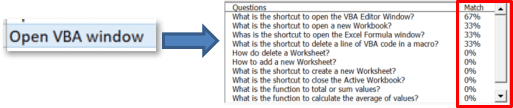
To show you how the Fuzzy Match VBA UserForm works I created a simple Knowledge Base of Excel/VBA related questions. The KB consists of 3 basis columns: Questions, Answer and Category. The Category column is especially useful as looking at the query you might want to limit the Fuzzy algorithm to run on only a subset of items in your database.

Designing the Fuzzy Match UserForm

Below a quick overview of the Fuzzy Match VBA UserForm if you want to see it in action:

Below you can find the design of the VBA Fuzzy Match UserForm.

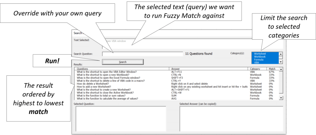
Each field is explained below:

• Text Selected – text from the Excel cell you selected in your workbook before running the VBA macro
• Search Question – if you want to override the “Text Selected” field simply type your query here and hit the Search button again. A typical scenario for this field is when you see that the result for your “Text Selected” don’t return satisfactory results and you would like to adjust the query
• Category(s) – if you want to improve the algorithm performance or simply reduce the categories to be searched then select the ones you are interested in
• Search – the Search button will run the algorithm and return results to the “Results” table
• Selected Question / Selected Answer – when you click on one of the results these fields will show the full text of the Question and Answer column. This makes it easier to copy the results where needed

The VBA Code

Initializing the UserForm

Firstly we will initialize our UserForm and assure it is showing us the current list of categories in our “KnowledgeBase” worksheet:

Private Sub UserForm_Initialize()
    Set catDict = GetListofCategories()
    For Each it In catDict.keys
        lbCategory.AddItem it
    Next it
    lbCategory.AddItem "Any"
    For i = 0 To lbCategory.ListCount - 1
        lbCategory.Selected(i) = True
    Next i
    tbSelectedQuestion.Text = Selection.Value
End Sub

Function GetListofCategories()
    Dim question As Range
    Set dict = CreateObject("Scripting.Dictionary")
    Set wsQnA = GetQnAWorksheet
    For Each question In wsQnA.Range("C:C").SpecialCells(xlCellTypeConstants)
        If question.Row > 1 Then
            If Not dict.Exists(question.Value) Then
                dict.Add question.Value, 1
            End If
        End If
    Next question
    Set GetListofCategories = dict
End Function

Function GetQnAWorksheet() As Worksheet
    Dim ws As Worksheet
    For Each ws In ActiveWorkbook.Sheets
        If ws.Name Like "KnowledgeBase*" And ws.Visible Then
            Set GetQnAWorksheet = ws
            Exit Function
        End If
    Next ws
    MsgBox "KnowledgeBase worksheet not found!~", vbCritical + vbOKOnly, "Error"
    Set GetQnAWorksheet = Nothing
End Function

Function for removing Stop Words

Before we focus on generating matches let us focus for a sec on creating a function that will remove stop words from a given sentence. This will help us get rid of all those unnecessary words like “the, it, this” etc. that will dilute the fuzzy algorithm.

Function RemoveStopWords(sentence As String) As Collection
    If IsEmpty(stopWords) Then stopWords = Split("a;about;above;after;again;against;all;am;an;and;any;are;aren't;as;at;be;because;been;before;being;below;between;both;but;by;can't;cannot;chat;could;couldn't;did;didn't;do;does;doesn't;doing;don't;down;during;each;few;for;from;further;had;hadn't;has;hasn't;have;haven't;having;he;he'd;he'll;he's;her;here;here's;hers;herself;hi;him;himself;his;how;how's;i;i'd;i'll;i'm;i've;if;in;into;is;isn't;it;it's;its;itself;let's;me;more;most;mustn't;my;myself;need;needs;no;nor;not;of;off;on;once;only;or;other;ought;our;ours;out;over;own;same;shan't;she;she'd;she'll;she's;should;shouldn't;so;some;such;than;that;that's;the;their;theirs;them;themselves;then;there;there's;these;they;they'd;they'll;they're;they've;this;those;through;to;too;under;until;up;very;was;wasn't;we;we'd;we'll;we're;we've;were;weren't;what;what's;when;when's;where;where's;which;while;who;who's;whom;why;why's;with;won't;would;wouldn't;you;you'd;you'll;you're;you've;your;yours;yourself;yourselves;?;!;" & _
             "-;,;", ";")
    Dim stopR As Range, r As Variant, col As Collection
    Set col = New Collection
    For Each w In Split(sentence, " ")
        If Not (IsNumeric(Trim(w))) Then
            w = Trim(w)
            If Len(w) > 0 Then col.Add w
        End If
    Next w
    For Each r In stopWords
        For i = col.Count To 1 Step -1
            If UCase(col(i)) = UCase(r) Then
                col.Remove i
            End If
        Next i
    Next r
    Set RemoveStopWords = col
End Function

You probably noticed I embedded a lot of words directly in the function. This makes it easy to add or remove stop words quickly.

Fuzzy Matching algorithm

Now for the meaty part :). Below the key logic for generating the results:

Public stopWords As Variant
Dim selectedChat As Range
Private Sub cbSearch_Click()
    'Clear Search worksheet
    Set selectedChat = Selection
    Dim wsRes As Worksheet: Set wsRes = GetSearchWorksheet
    selectedChat.Worksheet.Activate
    'Remove stop words from question
    Dim qCol As Collection
    Set qCol = RemoveStopWords(Selection.Value)
    'Search
    Dim wsQnA As Worksheet, r As Range, saCol As Collection, sa() As String, saIndex As Long
    Dim dict As Object, dstR As Range, startCount As Long, pMax As Long, currProgress As Long
    Set dict = CreateObject("Scripting.Dictionary")
    For i = 0 To lbCategory.ListCount - 1
        If lbCategory.Selected(i) Then
            dict.Add lbCategory.List(i), lbCategory.List(i)
        End If
    Next i
    'Search question matching Service Area, search query and calculate match
    Set wsQnA = GetQnAWorksheet
    If wsQnA Is Nothing Then Exit Sub
    startCount = wsRes.Range("A:A").SpecialCells(xlCellTypeConstants).Count
    pMax = wsQnA.Range("A:A").SpecialCells(xlCellTypeConstants).Count
    For Each r In wsQnA.Range("A:A").SpecialCells(xlCellTypeConstants)
        If dict.Exists(r.Offset(0, 4).Value) Or IsEmpty(r.Offset(0, 4).Value) And r.Row > 1 Then
            If tbSearch.Value = vbNullString Or InStr(1, r.Value, tbSearch.Value, vbTextCompare) > 0 Then
                Set dstR = wsRes.Range("A1").Offset(startCount):  startCount = startCount + 1
                dstR.Value = r.Value
                dstR.Offset(0, 1).Value = r.Offset(0, 1).Value
                dstR.Offset(0, 2).Value = r.Offset(0, 2).Value
                dstR.Offset(0, 3).Value = CalculateMatch(qCol, r.Value)
                dstR.Offset(0, 3).NumberFormat = "0%"
            End If
        End If
        currProgress = currProgress + 1
        If currProgress Mod 100 = 0 Then
            lStatus.Caption = "Searching " & Format(CDbl(currProgress) / pMax, "0%")
            DoEvents
        End If
    Next r
    'Display Search sorted by Match
    If wsRes.UsedRange.Rows.Count > 0 Then
        With wsRes.Sort
            .SortFields.Clear
            .SortFields.Add2 Key:=GetSearchLastColumn(wsRes), SortOn:=xlSortOnValues, Order:=xlDescending, DataOption:=xlSortNormal
            .SetRange wsRes.UsedRange
            .Header = xlYes
            .MatchCase = False
            .Orientation = xlTopToBottom
            .SortMethod = xlPinYin
            .Apply
        End With
    End If
    
    lbResult.RowSource = GetSearchRangeAddress(wsRes)
    lStatus.Caption = "" & lbResult.ListCount & " Questions found"
End Sub
Function GetSearchRangeAddress(ws As Worksheet)
    GetSearchRangeAddress = "'" & ws.Name & "'!" & Range(ws.Range("A2"), ws.Cells(ws.UsedRange.Rows.Count, ws.UsedRange.Columns.Count)).AddressLocal
End Function
Function GetSearchLastColumn(ws As Worksheet) As Range
    Set GetSearchLastColumn = Range(ws.Range("D2"), ws.Cells(ws.UsedRange.Rows.Count, ws.UsedRange.Columns.Count))
End Function

Function CalculateMatch(sentCol As Collection, sentence As String) As Double
    Dim m As Long, s() As String
    s = Split(sentence, " ")
    For Each w In sentCol
        For Each ws In s
            If UCase(ws) = UCase(w) Then
                m = m + 1
                Exit For
            End If
        Next ws
    Next w
    CalculateMatch = m / sentCol.Count
End Function
Sub CreateSearchResultsHeader(ws As Worksheet)
    ws.Range("A1").Value = "Questions"
    ws.Range("B1").Value = "Answer"
    ws.Range("C1").Value = "Category"
    ws.Range("D1").Value = "Match"
End Sub
Sub AddSearchResultsRow(ws As Worksheet, rowNum As Long, question As String, answer As String, sa As String, match As String)
    ws.Range("A" & rowNum).Value = question
    ws.Range("B" & rowNum).Value = answer
    ws.Range("C" & rowNum).Value = sa
    ws.Range("D" & rowNum).Value = match
End Sub
Function GetSearchWorksheet()
    Dim ws As Worksheet
    For Each ws In ActiveWorkbook.Sheets
        If ws.Name = "SearchResults" Then
            ws.UsedRange.Clear
            CreateSearchResultsHeader ws
            Set GetSearchWorksheet = ws
            Exit Function
        End If
    Next ws
    Set ws = ActiveWorkbook.Sheets.Add
    ws.Name = "SearchResults"
    CreateSearchResultsHeader ws
    Set GetSearchWorksheet = ws
End Function

The above code will do the following – compare the query to each question from the selected categories, calculate the match and add it to a temporary worksheet. Once done the table in the form will be connected to the range in the temporary worksheet and displayed.

Below a few other pieces of code that help display the Q/A in the text boxes and help us clean-up:

Private Sub lbResult_Click()
    'Display question and answer in textbox below
    For i = 0 To lbResult.ListCount - 1
        If lbResult.Selected(i) Then
            tbQ.Value = lbResult.List(i, 0)
            tbA.Value = lbResult.List(i, 1)
        End If
    Next i
End Sub

Private Sub UserForm_Terminate()
    On Error Resume Next
    Application.DisplayAlerts = False
    ActiveWorkbook.Sheets("SearchResults").Delete
    Application.DisplayAlerts = True
End Sub

Download the entire VBA Code Module

If you want to download the entire VBA Code Module for the Excel VBA Fuzzy Match UserForm click the download button below:
Download