
Одна из самых неприятных ситуаций, с которой может столкнуться пользователь при работе в Microsoft Excel — это поиск и подстановка данных с неточным совпадением. Когда вам надо подставить данные из одной таблицы в другую, но вы при этом уверены, что в обеих таблицах совпадающие элементы называются одинаково, то проблем нет — к вашим услугам множество способов: функции ВПР и её аналоги, надстройка Power Query и т.д.
А вот если в одной таблице «Пупкин Василий», а в другой просто «Пупкин», или «Пупкин В.», или даже «Пупкен», то все эти красивые способы не работают. Причем на практике такое встречается постоянно, особенно с почтовыми адресами или названиями компаний:

Обратите внимание на различные типы несоответствий, которые могут встречаться:
- переставлены местами улица, город, дом
- отсутствует какая-то часть адреса или, наоборот, есть что-то лишнее (индекс, номер квартиры)
- по-разному записан город (с буквой «г.» или без) или улица
- опечатки и ошибки (Козань вместо Казань)
Про точное соответствие или даже поиск по маске тут говорить не приходится. Помочь в таком случае могут только специальные макросы или надстройки для Excel. Про одну из таких макро-функций на VBA я уже писал, а здесь хочется рассказать про еще один вариант решения подобной задачи — надстройку Fuzzy Lookup от компании Microsoft.
Эта надстройка существует с 2011 года и совершенно бесплатно скачивается с сайта Microsoft. Системные требования: Windows 7 или новее, Office 2007 или новее, соответственно. После установки у вас в Excel появляется одноименная вкладка с единственной кнопкой на ней:

Нажатие на эту кнопку включает специальную панель в правой части окна Excel, где и задаются все настройки поиска:

Сразу хочу отметить, что эта надстройка умеет работать только с умными таблицами, поэтому все исходные таблицы нужно конвертировать в умные с помощью сочетания Ctrl+T или кнопки Форматировать как таблицу на вкладке Главная (Home — Format as Table):
Алгоритм действий при работе с надстройкой Fuzzy Lookup следующий:
- Выберите какие таблицы нужно связать в выпадающих списках Left и Right Table.
- Выберите ключевые столбцы в левой и правой таблицах, по которым нужно проверить соответствие и нажмите кнопку для добавления созданной пары в список Match Columns
- В списке Output Columns отметьте галочками столбцы, которые вы хотите получить на выходе в качестве результата.
- Установите активную ячейку в пустое место на листе, куда вы хотите вывести данные
- Нажмите кнопку Go
После анализа мы получаем таблицу, где каждому элементу ключевого столбца из первой таблицы подобрано максимально похожее значение из второй:

Лепота!
Нюансы и подводные камни
- Точность подбора можно регулировать с помощью ползунка Similarity Threshold в нижней части панели Fuzzy Lookup. Чем правее его положение, тем строже будет поиск, и — как следствие — тем меньше результатов надстройка будет находить. Если сдвинуть его влево, то результатов станет больше, но возрастет риск ошибочного совпадения. Тут все зависит от вашей конкретной ситуации — экспериментируйте.
- На больших таблицах поиск может занимать приличное количество времени (до нескольких десятков секунд), хотя многое, конечно, зависит от мощности вашего компьютера. Как вариант, для ускорения в настройках (кнопка Configure в нижней части панели) можно попробовать включить параметр UseApproximateIndexing в разделе Global Settings.
- Перед нажатием на кнопку Go не забудьте выделить пустую ячейку, начиная с которой вы хотите вывести результаты. Если случайно вы оставите активную ячейку где-нибудь в исходных данных, то надстройка выведет итоговую таблицу прямо поверх них, и вы их потеряете. Причем отмена последнего действия будет невозможна, а кнопка Undo в нижней части панели не всегда срабатывает почему-то.
- Для вывода столбца с коэффициентом подобия FuzzyLookup.Similarity необходимо, чтобы у вашего Excel была точка в качестве десятичного разделителя (целой и дробной части). Если это не так, то эту настройку временно можно поменять через Файл — Параметры — Дополнительно (File — Options — Advanced).
- Fuzzy Lookup — это не обычная надстройка, написанная на VBA (как мой PLEX, например), а COM-надстройка. Разница в том, что она устанавливается как отдельная программа, т.е. вам нужны соответствующие права на установку ПО на вашем компьютере. Дома, ясное дело, проблем не будет, а вот многим корпоративным пользователям, скорее всего, придется обращаться к вашим айтишникам. После установки отключать и подключать ее в дальнейшем можно на вкладке Разработчик — Надстройки COM (Developer — COM Add-ins).
В любом случае, при всех имеющихся минусах, эта надстройка однозначно стоит того, чтобы находиться в арсенале любого продвинутого пользователя Microsoft Excel.
Ссылки по теме
- Неточный поиск ближайшего похожего текста с помощью макрофункции
- Анализ текста регулярными выражениями (RegExp) в Excel
- Ссылка на скачивание надстройки Fuzzy Lookup с сайта Microsoft
ГлавнаяНечеткий поиск в Excel — Fuzzy Lookup Add-In for Excel
Нечеткий поиск — позволяет искать нечеткие соответствия текста в нескольких источниках.
Установочник:
https://www.microsoft.com/en-us/download/confirmation.aspx?id=15011
Скинуть на лист два источника, которые нужно сравнить.


1.
2.
3.
4.
5.
6. Перед нажатием GO — нужно на листе выбрать область куда выведется результат
Иправление возможной ошибки — меняем разделитель на точку.

Иногда нам нужно не только выполнить точный поиск, но и выполнить нечеткий поиск, как показано на скриншоте ниже. На самом деле в Excel функция «Найти и заменить» несколько помогает при нечетком поиске.
Нечеткий поиск с помощью поиска и замены
Нечеткий поиск одного или нескольких значений с помощью удобного инструмента
Образец файла
Предположим, у вас есть диапазон A1: B6, как показано на скриншоте ниже, вы хотите найти нечеткую строку поиска «яблоко» без учета регистра или приложения в этом диапазоне. Для выполнения задания можно применить функцию «Найти и заменить».

Искать без учета регистра
1. Выберите диапазон, который вы хотите найти, нажмите клавиши Ctrl + F , чтобы включить функцию Найти и заменить , введите строку, которую вы хотите найти, в Найдите текстовое поле.

2. Нажмите Параметры , чтобы развернуть диалоговое окно, снимите флажок Учитывать регистр , но установите флажок Сопоставить все содержимое ячейки .

3. Нажмите Найти все , строки перечислены без учета регистра.

Найти часть строки
1. Выберите диапазон и нажмите клавиши Ctrl + F , чтобы включить функцию Найти и заменить , и введите строку детали, которую вы хотите найти, в Найдите текстовое поле , снимите флажок Соответствовать всему содержимому ячейки , при необходимости также снимите флажок Учитывать регистр .

2. Нажмите Найти все , и будут перечислены ячейки, содержащие строку.

Нечеткий поиск одного значения или нескольких значений с помощью удобного инструмента
Если вам нужно найти примерно одно значение или узнать все приблизительные значения одновременно, вы можете использовать функцию Fuzzy Lookup в Kutools for Excel .
| Kutools for Excel , с более чем 300 удобными функциями, упрощает вашу работу. |
|
Бесплатная загрузка |
После бесплатной установки Kutools for Excel, сделайте следующее:
Найдите примерно одно значение
Предположим, вы хотите найти значение «app» в диапазоне A1: A7, но количество различных символов не может быть больше 2, а количество символов должно быть больше 1.

1. Нажмите Kutools > Найти > Нечеткий поиск , чтобы включить панель Нечеткий поиск .

2. На всплывающей панели выполните следующие действия:
1) Выберите диапазон, который вы использовали для поиска, вы можете установить флажок Указано , чтобы исправить диапазон поиска.
2) Установите флажок Найти по указанному тексту .
3) Введите значение, на основе которого вы хотите выполнять нечеткий поиск, в Text .
4) Укажите необходимые критерии поиска.

3. Нажмите кнопку Найти , затем нажмите стрелку вниз, чтобы развернуть список и просмотреть результаты поиска.

Нечеткий поиск нескольких значений
Предположим, вы хотите найти все приблизительные значения в диапазоне A1: B7, вы можете сделать следующее:

1. Нажмите Kutools > Найти > Нечеткий поиск , чтобы включить панель Нечеткий поиск .
2. На панели Нечеткий поиск выберите диапазон поиска, а затем укажите необходимые критерии поиска.

3. Нажмите кнопку Найти , чтобы перейти к просмотру результатов поиска, затем нажмите стрелку вниз, чтобы развернуть список.

Быстрое разделение данных на несколько листов на основе столбца или фиксированных строк в Excel
|
| Предположим, у вас есть рабочий лист с данными в столбцах A на G имя продавца находится в столбце A, и вам необходимо автоматически разделить эти данные на несколько листов на основе столбца A в той же книге, и каждый продавец будет разделен на новый рабочий лист. Kutools for Excel может помочь вам быстро разделить данные на несколько листов на основе выбранного столбца, как показано на скриншоте ниже в Excel. Нажмите, чтобы получить 60-дневную бесплатную пробную версию! |
 |
| Kutools for Excel: с более чем 300 удобными надстройками Excel, бесплатно и без ограничений в течение 30 дней. |
Образец файла
Щелкните, чтобы загрузить образец файла
Другие операции (статьи)
Найти наибольшее отрицательное значение (меньше 0) в Excel
Для большинства пользователей Excel найти наибольшее значение из диапазона очень легко, но как насчет поиска наибольшего отрицательного значения (меньше чем 0) из диапазона данных, смешанного с отрицательными и положительными значениями?
Найти наименьший общий знаменатель или наибольший общий знаменатель в Excel
Все мы, возможно, помним, что в студенческие годы нас просили вычислить наименьший общий знаменатель или наибольший общий знаменатель некоторых чисел. Но если их десять или больше и несколько больших чисел, эта работа будет сложной.
Пакетный поиск и замена определенного текста в гиперссылках в Excel
В Excel вы можете выполнить пакетную замену определенной текстовой строки или символа в ячейках другим с помощью функции «Найти и заменить». Однако в некоторых случаях вам может потребоваться найти и заменить определенный текст в гиперссылках, исключая другие форматы содержимого.
Примените Функция обратного поиска или поиска в Excel
Как правило, мы можем применить функцию поиска или поиска для поиска определенного текста слева направо в текстовой строке по определенному разделителю. Если вам нужно перевернуть функцию поиска, чтобы найти слово, начинающееся в конце строки, как показано на следующем снимке экрана, как вы могли бы это сделать?
Другие статьи
Инструменты повышения производительности Excel -> ->
The mapping of 301 redirects is an essential albeit often time-consuming SEO task. If you fail to compile and deploy a comprehensive redirect map during a site migration, then the results can be nothing short of catastrophic from an organic traffic / visibility perspective.
Working with large enterprise clients, it’s not uncommon for such websites to features tens of thousands of pages. Such page counts can often be further inflated if an organisation operates internationally across numerous territories and provides content in multiple languages.
In this post I’m going to detail how using Microsoft’s Fuzzy Lookup add-in for Excel could save you significant time (and your sanity) when compiling large redirect maps.
What is a fuzzy lookup
Firstly, what is Microsoft’s Fuzzy Look-Up add-in? The add-in was developed by Microsoft Research to allow the ‘fuzzy’ matching of textual data. It can be utilised to identify fuzzy matching rows both within a single table or to fuzzy join rows across two different tables within Excel. Where fuzzy lookup differs from a standard vlookup, hlookup or index match type formula is its ability to more robustly match rows in the presence of spelling mistakes, abbreviations, synonyms and added / missing data. A further benefit is the ability for the add-in to generate a similarity score allowing for a confidence level to be factored in.
Before we get started, click here to download Microsoft’s Fuzzy Lookup Excel Plugin.
Step 1 – Compile website crawls
Once you have completed installation of the Fuzzy Lookup add-in for Excel, the first task which you must complete is to perform a crawl of both the live (legacy) website and the staging (new) website.
Choosing a crawl tool
To perform this task, you can utilise a host of site crawling tools including: Screaming Frog, DeepCrawl, Moz, Ahrefs. Each tool has their own respective benefits, but my personal preference would be either Screaming Frog or DeepCrawl. The key determining factor for which tool to use is likely to be primarily driven by the size of your site. Screaming Frog is a powerful offline crawl tool which you install on your own machine. It’s performance and ultimately the total number of URLs it can crawl is very much dependent on the spec of your machine. In contrast DeepCrawl is a cloud-based crawl tool which in theory has no limit on the number of URLs it can crawl. In order to utilise Screaming Frog on large enterprise sites then it is best to install it on a dedicated server. The cost of setting up such an environment is likely to outweigh the savings of the initial subscription fee.
From a cost perspective both tools in my opinion offer fantastic value for the functionality they provide. Screaming Frog offers a free version which can be run on sites <500 URLs, with an annual cost of £149 for the unlimited version. In comparison DeepCrawl starts at a monthly cost of £63 per month allowing you to crawl up to 100,000 URLs across 5 separate projects.
In summary if your website features 10,000 URLs or less then Screaming Frog is likely to be your best option, however if you have a website which exceeds this figure then DeepCrawl is likely to be the more cost-effective option in the long run.
Crawl prerequisites
Prior to running a crawl of both the current live website and new staging website, it is crucial to ensure:
- No future content updates are planned to be added to the current live website ahead of the new site launch. If any new pages are added after the crawl has been completed, then it is likely this content will be missed form the redirect map.
- All pages must have been created and ideally populated with content on the new staging website, specifically the following elements: URL, page title and H1(s)
Step 2 – Format data
Once separate crawls have been captured / exported for both the current live website and new staging website, the next step is to remove all unnecessary data. Optimally only the following information is required:
- URL
- Page title
- H1
Legacy crawl
The screenshot below illustrates a sample selection of URLs / content which will act as our current live site:
Staging crawl
This second screenshot illustrates a sample selection of URLs / content captured from our proposed new staging website:
Notice the updated URLs, optimised page titles and refined H1 content.
Once all unnecessary data has been deleted from each respective crawl, copy and paste each crawl into a single document but on to separate tabs – ‘Source’ and ‘Destination’. Additionally, create a third empty tab and name it ‘Redirect Map’. It is this tab where we will compile the final output.

Next format the data from both crawls as a table within their respective tabs. Each table should be given a logical name to ensure they can be easily differentiated when utilising the fuzzy lookup function. ‘liveSite’ and ‘stagingSite’ are the respective table names I will utilise for the purposes of this tutorial. For reference table names must be absent of spaces, so I utilise camel case naming conventions to aid readability.

Step 3 – Perform Fuzzy Lookup(s)
Once you have compiled all crawl data the next step is to begin the actual redirect mapping activity. To begin, open the Fuzzy Lookup sidebar by clicking the Fuzzy Lookup option within Excel’s ribbon.

Create table join
The first step to performing a fuzzy lookup is to create a join (relationship) between your live website crawl (Left Table) and new staging website crawl (Right Table). In the ‘Left Table’ drop down menu select the table named ‘liveSite’ and in the ‘Right Table’ drop down menu select the table named StagingSite’.
Once both tables have been selected, you must now define which columns should be specifically matched within the fuzzy lookup function. Columns are selected by choosing the respective column headers from the drop-down list and then clicking the connect button. Note it may be necessary to delete existing predefined auto-generated column relationships from the ‘Match Columns’ list.
Dependent on your actual data is likely to influence which columns you utilise within your fuzzy lookup function(s). I typically begin by trying the H1. H1s tend to feature the most refined / optimally matchable data. However no two sites are the same so the key here is trial and error until you achieve the optimum result:
Select output columns
In order to produce a redirect map requires a source URL and a destination URL. As such for the output columns select: ‘liveSite.URL’ and ‘stagingSite.URL’.
Additionally select to output the following column ‘FuzzyLookup.Similarity’ (more on this later).
Define number of matches
Next define the number of matches to return per input row. The value should be left unchanged as ‘1’:

Similarity threshold
The similarity threshold allows you to adjust the sensitivity of the fuzzy matching. Typically I would recommend starting in the default position of ‘0.5’ and then adjusting up and down accordingly. Helpfully included within the sidebar is an undo button which you can quickly press to reset the output each time a new configuration is trialed:

Go
The final step prior to hitting ‘Go’ is to place your cursor where you wish the output to be inserted. For the purposes of this tutorial select cel A1 on the ‘Redirect Map’ tab which you previously created.
Step 4 – The Output
The screenshots below illustrate the respective outputs from matching each of the different columns. Notice the varying similarity scores across each column:
H1 match
Page title match
URL match
Step 5 – Manual Checks
It is import to note that you will be left with a requirement to perform manual checks as it is almost certain not all pages will be optimally matched. For example closely related pages may inadvertently be matched to a page which while similar is not be the best / true match. To aid analysis of results you can order the output of results within your newly created redirect map by the output similarity score. The higher the similarity score the greater the confidence of the result. Any score <0.5 is almost certainly likely to require further investigation.
Additional Steps (Performance Enhancements)
While the implementation of redirects is essential to help maintain organic visibility / promote optimum usability, it is also important to carefully consider the respective performance implications. Redirect rules have a direct impact on page speed due to the requirement for a server to check all redirect rules prior to loading a web page. The greater the number of redirects, the more time will be required to parse all respective redirect rules. For this reason it is crucial to rationalise any redirect list prior to uploading in order to ensure it does not contain potential bloat.
In order to help rationalise your redirect map I would strongly recommended both analytics data and authority data is also factored into your redirect map creation methodology. Analytics data should be utilised to exclude pages which have received low entrances or page views. Common sources include: Google Analytics, Adobe Analytics Cloud etc. Similarly authority data should be utilised to help prioritise the inclusion of redirects based on perceived levels of authority held by a page. In order to help identify such levels of authority I would recommend factoring a metric such as Moz’s Page Authority (PA).
Finally in addition to rationalising your redirect map, further potential performance gains can be achieved through the utilisation of pattern matching rules implemented via regular expressions, commonly referred to as regex. A regular expression is a string that describes or matches a set of strings. In the case of redirects, a single regular expression can be utilised to match a set of pages which match a defined criteria. This can enable the number of rules contained within a redirect map to be significantly reduced enabling a server to process it in a reduced amount of time, promoting fast page load times.
We can use Excel Fuzzy Lookup Add-In to match similar, but not exactly matching data. FUZZY LOOKUP returns a table of matched similar data in the chosen column. FUZZY LOOKUP is useful for comparing two same data sets where one of them comes from an external source and can be misspelled or typed incorrectly. This article will guide all levels of excel users on how to use FUZZY LOOKUP.
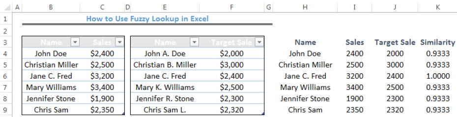 Figure 1- How to Use Fuzzy Lookup in Excel
Installation of Fuzzy Lookup in Excel
You won’t find FUZZY LOOKUP in the standard excel tabs and buttons. Download it by clicking HERE and follow the installation instructions.
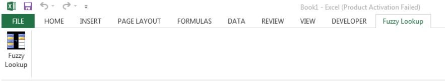 Figure 2- Fuzzy Lookup Installed In Excel
Creation of Fuzzy Lookup Table with the Data
We must format our data into tables to use Fuzzy Lookup.
- To do this, we will select the cell range for each table
- We will click on Insert tab and choose Table
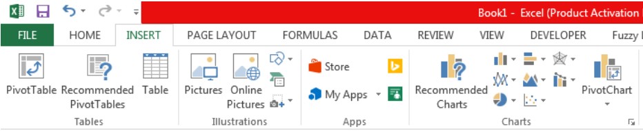 Figure 3- Creation of Fuzzy Lookup Table with the Data
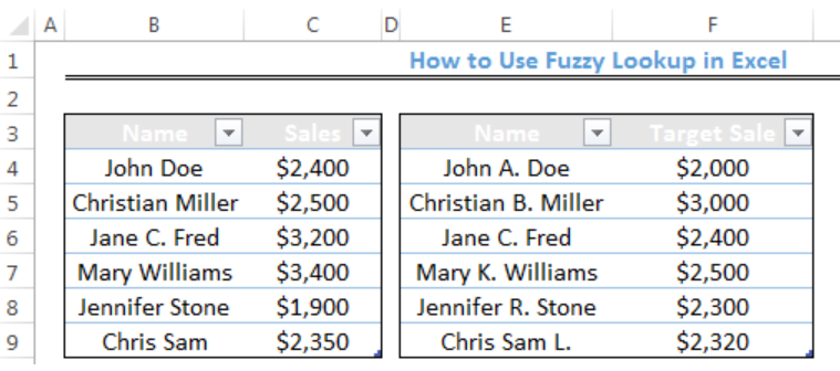 Figure 4- Creation of Fuzzy Lookup Table with the Data
After we have created the two tables, we need to name them to enable their use by Fuzzy Lookup function. We do this by selecting the whole table and enter a name into the Name Box. The name box is where we have H5 in figure 5.
We will enter Sales as the name of the first table and Target Sales for the second table.
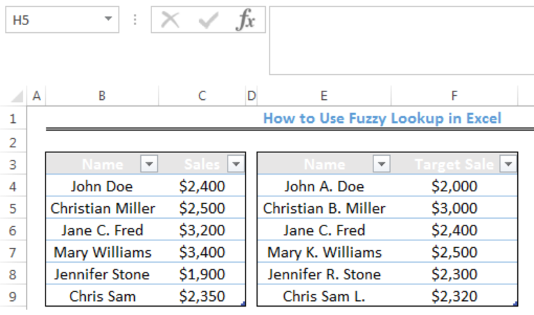 Figure 5- Naming the tables for Fuzzy Lookup Use
Using the FUZZY LOOKUP Function
Our aim is to use the fuzzy lookup function to match Name in the first table with Sales in the first table including target sales in the second table based on their similarity. We are assuming that the names in the second table aren’t spelled correctly.
- First, we will click on Cell H3 where our new table will begin
- We will click on Fuzzy lookup and click on Fuzzy Lookup below file
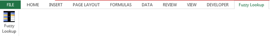 Figure 6- Using the FUZZY LOOKUP Function
- For the output column, we will check the following boxes: Table1.Name, Table1.Sales, Table2.Target Sale, and FuzzyLookup.Similarity
- We will set the Similarity Threshold as 0.9
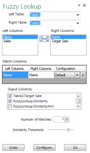 Figure 7- Using the FUZZY LOOKUP Function
- We will click Go
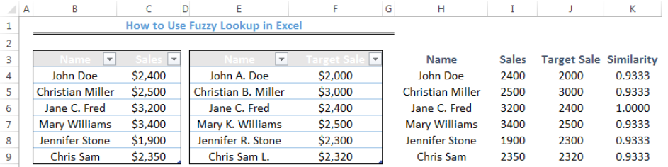 Figure 8- Result of the Fuzzy Lookup Function
Instant Connection to an Expert through our Excelchat Service
Most of the time, the problem you will need to solve will be more complex than a simple application of a formula or function. If you want to save hours of research and frustration, try our live Excelchat service! Our Excel Experts are available 24/7 to answer any Excel question you may have. We guarantee a connection within 30 seconds and a customized solution within 20 minutes.