
Одна из самых неприятных ситуаций, с которой может столкнуться пользователь при работе в Microsoft Excel — это поиск и подстановка данных с неточным совпадением. Когда вам надо подставить данные из одной таблицы в другую, но вы при этом уверены, что в обеих таблицах совпадающие элементы называются одинаково, то проблем нет — к вашим услугам множество способов: функции ВПР и её аналоги, надстройка Power Query и т.д.
А вот если в одной таблице «Пупкин Василий», а в другой просто «Пупкин», или «Пупкин В.», или даже «Пупкен», то все эти красивые способы не работают. Причем на практике такое встречается постоянно, особенно с почтовыми адресами или названиями компаний:

Обратите внимание на различные типы несоответствий, которые могут встречаться:
- переставлены местами улица, город, дом
- отсутствует какая-то часть адреса или, наоборот, есть что-то лишнее (индекс, номер квартиры)
- по-разному записан город (с буквой «г.» или без) или улица
- опечатки и ошибки (Козань вместо Казань)
Про точное соответствие или даже поиск по маске тут говорить не приходится. Помочь в таком случае могут только специальные макросы или надстройки для Excel. Про одну из таких макро-функций на VBA я уже писал, а здесь хочется рассказать про еще один вариант решения подобной задачи — надстройку Fuzzy Lookup от компании Microsoft.
Эта надстройка существует с 2011 года и совершенно бесплатно скачивается с сайта Microsoft. Системные требования: Windows 7 или новее, Office 2007 или новее, соответственно. После установки у вас в Excel появляется одноименная вкладка с единственной кнопкой на ней:

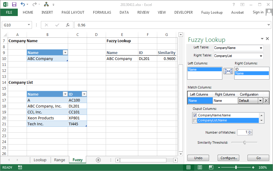
Нажатие на эту кнопку включает специальную панель в правой части окна Excel, где и задаются все настройки поиска:

Сразу хочу отметить, что эта надстройка умеет работать только с умными таблицами, поэтому все исходные таблицы нужно конвертировать в умные с помощью сочетания Ctrl+T или кнопки Форматировать как таблицу на вкладке Главная (Home — Format as Table):
Алгоритм действий при работе с надстройкой Fuzzy Lookup следующий:
- Выберите какие таблицы нужно связать в выпадающих списках Left и Right Table.
- Выберите ключевые столбцы в левой и правой таблицах, по которым нужно проверить соответствие и нажмите кнопку для добавления созданной пары в список Match Columns
- В списке Output Columns отметьте галочками столбцы, которые вы хотите получить на выходе в качестве результата.
- Установите активную ячейку в пустое место на листе, куда вы хотите вывести данные
- Нажмите кнопку Go
После анализа мы получаем таблицу, где каждому элементу ключевого столбца из первой таблицы подобрано максимально похожее значение из второй:

Лепота!
Нюансы и подводные камни
- Точность подбора можно регулировать с помощью ползунка Similarity Threshold в нижней части панели Fuzzy Lookup. Чем правее его положение, тем строже будет поиск, и — как следствие — тем меньше результатов надстройка будет находить. Если сдвинуть его влево, то результатов станет больше, но возрастет риск ошибочного совпадения. Тут все зависит от вашей конкретной ситуации — экспериментируйте.
- На больших таблицах поиск может занимать приличное количество времени (до нескольких десятков секунд), хотя многое, конечно, зависит от мощности вашего компьютера. Как вариант, для ускорения в настройках (кнопка Configure в нижней части панели) можно попробовать включить параметр UseApproximateIndexing в разделе Global Settings.
- Перед нажатием на кнопку Go не забудьте выделить пустую ячейку, начиная с которой вы хотите вывести результаты. Если случайно вы оставите активную ячейку где-нибудь в исходных данных, то надстройка выведет итоговую таблицу прямо поверх них, и вы их потеряете. Причем отмена последнего действия будет невозможна, а кнопка Undo в нижней части панели не всегда срабатывает почему-то.
- Для вывода столбца с коэффициентом подобия FuzzyLookup.Similarity необходимо, чтобы у вашего Excel была точка в качестве десятичного разделителя (целой и дробной части). Если это не так, то эту настройку временно можно поменять через Файл — Параметры — Дополнительно (File — Options — Advanced).
- Fuzzy Lookup — это не обычная надстройка, написанная на VBA (как мой PLEX, например), а COM-надстройка. Разница в том, что она устанавливается как отдельная программа, т.е. вам нужны соответствующие права на установку ПО на вашем компьютере. Дома, ясное дело, проблем не будет, а вот многим корпоративным пользователям, скорее всего, придется обращаться к вашим айтишникам. После установки отключать и подключать ее в дальнейшем можно на вкладке Разработчик — Надстройки COM (Developer — COM Add-ins).
В любом случае, при всех имеющихся минусах, эта надстройка однозначно стоит того, чтобы находиться в арсенале любого продвинутого пользователя Microsoft Excel.
Ссылки по теме
- Неточный поиск ближайшего похожего текста с помощью макрофункции
- Анализ текста регулярными выражениями (RegExp) в Excel
- Ссылка на скачивание надстройки Fuzzy Lookup с сайта Microsoft
Содержание
- Нечеткий текстовый поиск с Fuzzy Lookup в Excel
- Нюансы и подводные камни
- Perform Approximate Match and Fuzzy Lookups in Excel
- Understanding Built-In Lookup Functions
- The Truth about the VLOOKUP Fourth Argument
- What is a Fuzzy Lookup aka Approximate Match
- Add-In
Нечеткий текстовый поиск с Fuzzy Lookup в Excel
Одна из самых неприятных ситуаций, с которой может столкнуться пользователь при работе в Microsoft Excel — это поиск и подстановка данных с неточным совпадением. Когда вам надо подставить данные из одной таблицы в другую, но вы при этом уверены, что в обеих таблицах совпадающие элементы называются одинаково, то проблем нет — к вашим услугам множество способов: функции ВПР и её аналоги, надстройка Power Query и т.д.
А вот если в одной таблице «Пупкин Василий», а в другой просто «Пупкин», или «Пупкин В.», или даже «Пупкен», то все эти красивые способы не работают. Причем на практике такое встречается постоянно, особенно с почтовыми адресами или названиями компаний:
Обратите внимание на различные типы несоответствий, которые могут встречаться:
- переставлены местами улица, город, дом
- отсутствует какая-то часть адреса или, наоборот, есть что-то лишнее (индекс, номер квартиры)
- по-разному записан город (с буквой «г.» или без) или улица
- опечатки и ошибки (Козань вместо Казань)
Про точное соответствие или даже поиск по маске тут говорить не приходится. Помочь в таком случае могут только специальные макросы или надстройки для Excel. Про одну из таких макро-функций на VBA я уже писал, а здесь хочется рассказать про еще один вариант решения подобной задачи — надстройку Fuzzy Lookup от компании Microsoft.
Эта надстройка существует с 2011 года и совершенно бесплатно скачивается с сайта Microsoft. Системные требования: Windows 7 или новее, Office 2007 или новее, соответственно. После установки у вас в Excel появляется одноименная вкладка с единственной кнопкой на ней:
Нажатие на эту кнопку включает специальную панель в правой части окна Excel, где и задаются все настройки поиска:
Сразу хочу отметить, что эта надстройка умеет работать только с умными таблицами, поэтому все исходные таблицы нужно конвертировать в умные с помощью сочетания Ctrl + T или кнопки Форматировать как таблицу на вкладке Главная (Home — Format as Table) :
Алгоритм действий при работе с надстройкой Fuzzy Lookup следующий:
- Выберите какие таблицы нужно связать в выпадающих списках Left и Right Table.
- Выберите ключевые столбцы в левой и правой таблицах, по которым нужно проверить соответствие и нажмите кнопку для добавления созданной пары в список Match Columns
- В списке Output Columns отметьте галочками столбцы, которые вы хотите получить на выходе в качестве результата.
- Установите активную ячейку в пустое место на листе, куда вы хотите вывести данные
- Нажмите кнопку Go
После анализа мы получаем таблицу, где каждому элементу ключевого столбца из первой таблицы подобрано максимально похожее значение из второй:
Нюансы и подводные камни
- Точность подбора можно регулировать с помощью ползунка Similarity Threshold в нижней части панели Fuzzy Lookup. Чем правее его положение, тем строже будет поиск, и — как следствие — тем меньше результатов надстройка будет находить. Если сдвинуть его влево, то результатов станет больше, но возрастет риск ошибочного совпадения. Тут все зависит от вашей конкретной ситуации — экспериментируйте.
- На больших таблицах поиск может занимать приличное количество времени (до нескольких десятков секунд), хотя многое, конечно, зависит от мощности вашего компьютера. Как вариант, для ускорения в настройках (кнопка Configure в нижней части панели) можно попробовать включить параметр UseApproximateIndexing в разделе Global Settings.
- Перед нажатием на кнопку Goне забудьте выделить пустую ячейку, начиная с которой вы хотите вывести результаты. Если случайно вы оставите активную ячейку где-нибудь в исходных данных, то надстройка выведет итоговую таблицу прямо поверх них, и вы их потеряете. Причем отмена последнего действия будет невозможна, а кнопка Undo в нижней части панели не всегда срабатывает почему-то.
- Для вывода столбца с коэффициентом подобия FuzzyLookup.Similarity необходимо, чтобы у вашего Excel была точка в качестве десятичного разделителя (целой и дробной части). Если это не так, то эту настройку временно можно поменять через Файл — Параметры — Дополнительно (File — Options — Advanced) .
- Fuzzy Lookup — это не обычная надстройка, написанная на VBA (как мой PLEX, например), а COM-надстройка. Разница в том, что она устанавливается как отдельная программа, т.е. вам нужны соответствующие права на установку ПО на вашем компьютере. Дома, ясное дело, проблем не будет, а вот многим корпоративным пользователям, скорее всего, придется обращаться к вашим айтишникам. После установки отключать и подключать ее в дальнейшем можно на вкладке Разработчик — Надстройки COM (Developer — COM Add-ins) .
В любом случае, при всех имеющихся минусах, эта надстройка однозначно стоит того, чтобы находиться в арсенале любого продвинутого пользователя Microsoft Excel.
Источник
Perform Approximate Match and Fuzzy Lookups in Excel
This post explores Excel’s lookup functions, approximate matches, fuzzy lookups, and exact matches. The built-in Excel lookup functions, such as VLOOKUP, are amazing. When implemented in the right way for special projects or in recurring use workbooks, they are able to save a ton of time. The VLOOKUP function alone has saved countless hours in my recurring use workbooks. However, the VLOOKUP function, similar to Excel’s other lookup functions such as HLOOKUP and MATCH, is built to perform an exact match or a range lookup. Both of these are quite different from an approximate match or a fuzzy lookup. This post discusses the details of these ideas, and demonstrates how to perform a fuzzy lookup in Excel 2010 and later.
Understanding Built-In Lookup Functions
The built-in Excel lookup functions, such as VLOOKUP, HLOOKUP, and MATCH, work with similar lookup logic. To simplify this post, we’ll use just one as the example. Since the VLOOKUP function is probably the most used and most familiar lookup function, we’ll use it as we explore these ideas.
The basic idea of an Excel lookup function is to look for a value in a list. For example, we could ask Excel to find “ABC Company” in a list of customer names. That is the basic idea, but the application of lookup functions are numerous and the implementations can become quite sophisticated and powerful.
For this post, I’d like to split the tasks that a lookup function performs into two steps. I’ll call step one the match, and step two the return. In the first step, the match, Excel must find the matching value. You tell Excel the value to find, such as “ABC Company” and you tell Excel where to look, such as in a range of cells. You are asking Excel to find the lookup value in the lookup range.
Step two, the return, is the function’s result. That is, what value the function should return to the cell. Some lookup functions, such as the MATCH function, tell Excel to return the position number. Other lookup functions, such as the VLOOKUP function, tell Excel to return a related value. So, based on which lookup function you select, and which function argument values you enter, Excel knows what to return once it finds its match. So far so good?
Let’s do a quick example at this point.
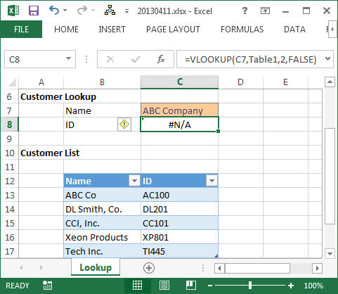
I would like to find a specific customer name “ABC Company” in a list of customers, and if found, I would like Excel to return the customer id which is found in the next column.
I would use a VLOOKUP function, and I would ask it to find “ABC Company” in the Customer Table, and return the ID. Assuming the customer name was entered in C7, and the customers were stored in a Table named Table1, then the following function would do the trick:
=VLOOKUP(C7, Table1, 2, FALSE)
Where:
- C7 is the value to find
- Table1 is the lookup range
- 2 is the column that has the value we wish to return
- FALSE means we are not performing a range lookup
This function is entered in C8 in the screenshot below.

As you can see, the ID AC100 was successfully returned to the formula cell C8. And that my friend is the basic idea of the VLOOKUP function. Find a value (the match) and compute the result (the return).
It is important to note that the lookup value, the text string “ABC Company” must be found in the lookup range. Except for case (upper and lower), the two values must match exactly. “ABC Company” would not match “ABC Company, Inc.”, “ABC Co”, or “ABC Company “. No leading spaces, no trailing spaces, no extra abbreviations or characters. They must be the same. This is called an exact match. If the value is not the same, the function will not match it, and you’ll get an error, as shown in the screenshot below.
Now that we have covered the basics, it is time to explore the VLOOKUP’s fourth argument.
The Truth about the VLOOKUP Fourth Argument
The fourth argument of the VLOOKUP function is officially named: range_lookup. It is a boolean argument, meaning you can pass it a value of TRUE or FALSE, or any other representation of TRUE or FALSE. The thing that tends to mislead Excel users is the description that Microsoft used for these options. Excel describes the TRUE value as “Approximate Match” and FALSE as “Exact Match.” A clearer description would have been something like TRUE “You are doing a range lookup” and FALSE “You are not doing a range lookup” but in any event, the descriptions are what they are.
When you select TRUE (Approximate Match) you are not asking Excel to match values that are approximately the same as each other. The description Approximate Match would tend to imply that the function would match “ABC Company” and “ABC Company, Inc.” since they are approximately the same name. In some cases and in some data sets, this idea would work. But this idea does not work in all cases, and thus, can’t be relied upon in our workbooks. For example, in the screenshot below, the function did not find a match between “ABC Company” and “ABC Company, Inc.” as evidenced by the incorrect ID returned in C8:
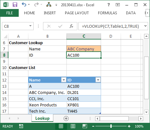
In the following screenshot however, the function did find a match between “ABC Company” and “ABC Co” as evidenced by the expected ID returned to C8:
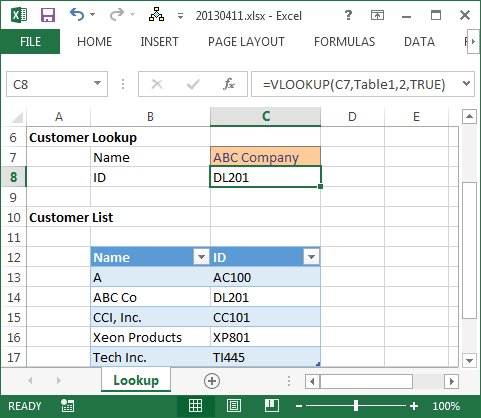
The way that the function actually works when TRUE is selected is this: it walks down the list row by row, and ultimately stops on the row that is less than the value and where the next row is greater than the value. This is why the lookup range must be sorted in ascending order for the function to return an accurate result when the fourth argument is TRUE.
This idea can be confusing when thinking about text strings, but makes more sense when thinking about numbers. For example, when trying to find the correct commission rate based on the sales value. In this case, you want to perform a range lookup. You want to look up a value from within a range. This is illustrated in the screenshot below.
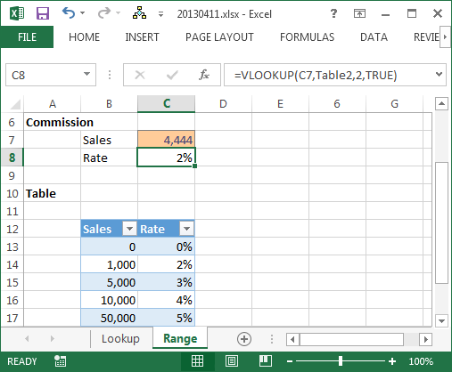
The function walks down row by row trying to determine which row to stop on. It continues down until it finds a row that is greater than the lookup value, and then it stops on the previous row. It stops on the row that is less than the value, and where the next row is greater than the lookup value. This is pretty easy to understand when thinking about numbers, but can be harder to visualize when thinking about text strings. The key to understanding this function argument however, is to realize that the logic is identical when operating on text strings and numbers. This is why “ABC Company” does not match “ABC Company, Inc.”, because “ABC Company Inc.” is greater than ABC Company. This is why “ABC Company” will match “ABC Co”, because “ABC Co” is less than “ABC Company.” As you can see, this is not what we have in mind when thinking about approximate match.
What is a Fuzzy Lookup aka Approximate Match
An approximate match, to us, means that two text strings that are about the same, but not necessarily identical, should match. For example, “ABC Company” should match “ABC Company, Inc.,” “ABC Co,” and “ABC Company .” We think about an approximate match as kind of fuzzy, where some of the characters match but not all.
The idea of a fuzzy lookup is that the values are not a clear match, they are not identical. But that they are likely a match, there is a probability that they are a match. They likely represent the same underlying entity.
Now that we realize the VLOOKUP function does not truly perform approximate match logic, at least, not in the way we want it, what do we do?
Add-In
When you hit a wall, go around it. Since the built-in lookup functions do not perform fuzzy logic when performing the match, we hit a built-in limitation of Excel. Microsoft has offered a way to work around this limitation by offering a free add-in.
Microsoft offers a free add-in that enables Excel to perform fuzzy lookups. It is called “Fuzzy Lookup Add-In for Excel” and is available at the time of this post at the link below:
Once installed, this add-in performs fuzzy lookups. It does not change the behavior of any of the built-in lookup functions. It does not enable your VLOOKUP functions to perform fuzzy lookups. It is an add-in which basically processes two lists and computes the probability of a match.
You specify the two tables, and within each table the columns to inspect. Basically, you define step one the match. You then define step two by identifying which columns from the tables should be included in the result. You can also specify the probability threshold. You hit go, and the add-in performs its work, and then outputs the resulting table starting at the active cell. It basically generates a static report based on the settings you select.
Here is a screenshot of the output, showing that it successfully matched “ABC Company” and “ABC Company, Inc.” in the same data set that caused our VLOOKUP function to fail.
For more information about the fuzzy lookup add-in, and more detail on how to use it, please visit the Microsoft link above. The add-in comes with instructions, a sample Excel file, and a pdf file with background and the logic it uses to do its magic. It also comes with a license, so, you’ll want to be sure to read the license terms in the LicenseTerms.rtf document included with the download.
There is some extremely interesting computer science and math working behind the scenes, including Jaccard similarity, tokenization of records, and transformations. Pretty heavy mathematics in there. Thanks Microsoft Research for this add-in!!
Источник
ГлавнаяНечеткий поиск в Excel — Fuzzy Lookup Add-In for Excel
Нечеткий поиск — позволяет искать нечеткие соответствия текста в нескольких источниках.
Установочник:
https://www.microsoft.com/en-us/download/confirmation.aspx?id=15011
Скинуть на лист два источника, которые нужно сравнить.


1.
2.
3.
4.
5.
6. Перед нажатием GO — нужно на листе выбрать область куда выведется результат
Иправление возможной ошибки — меняем разделитель на точку.

Skip to content
Ищем похожие записи и приблизительные совпадения
Быстрый способ выполнить приблизительный поиск в Excel
Используйте Fuzzy Duplicate Finder для поиска и исправления опечаток в таблицах Excel. Надстройка выполняет поиск частичных дубликатов, которые отличаются на от 1 до 10 символов, и распознает пропущенные, лишние или ошибочные символы. Вы просто выбираете, что исправить, делаете пару щелчков мышью и получаете в свое распоряжение исправленный набор данных.
-
60-дневная безусловная гарантия возврата денег
-
Бесплатные обновления на 2 года
-
Бесплатная и бессрочная техническая поддержка
С помощью инструмента поиска Fuzzy Duplicate Finder вы сможете:
Искать в нескольких строках и столбцах
Найдите все похожие значения, которые отличаются от 1 до 10 символов.
Управляйте правильными вариантами написания
Замените найденные опечатки одним из слов из списка встречающихся вариантов или введите собственное наиболее правильное значение.
Быстро переходить между результатами поиска
Все найденные совпадения организованы по группам в зависимости от степени и характера совпадения.
Экспорт найденных опечаток
Экспортируйте результаты поиска на отдельный рабочий лист для просмотра или исправления.

Что такое инструмент поиска похожих записей и для чего он мне нужен?
Fuzzy Duplicate Finder для Excel может помочь вам найти и исправить всевозможные частичные дубликаты, опечатки и слова с ошибками на ваших листах. Инструмент выполняет поиск нечетких дубликатов, которые отличаются на 1 — 10 символов, и распознает пропущенные, лишние или ошибочные символы. Это позволяет автоматически или вручную исправлять ошибки ввода и опечатки прямо в результатах поиска.
Почему бы не использовать программу проверки орфографии Excel для исправления опечаток?
Встроенная в Excel программа проверки орфографии и грамматики ищет только очевидные ошибки. Он не найдет все варианты с одним и тем же именем и не покажет вам список всех этих нечетких совпадений. Ведь опечатка или ошибка могут быть вполне орфографически правильны, но по смыслу — совершенно неверны. Более того, в стандартном словаре Excel может просто не хватать нужного вам значения.
А как насчет надстройки Microsoft Fuzzy Lookup для Excel?
Надстройка Fuzzy Lookup от Microsoft работает только в Excel 2007–2013 и может сравнивать данные только в двух похожих наборах данных, отформатированных в виде таблиц.
Эта же надстройка работает с любой версией Excel 2019, 2016–2010, а также Office 365, поддерживает все версии Windows и может обрабатывать любой диапазон ячеек независимо от его формата.
Как работает Fuzzy Duplicate Finder?
Инструмент позволяет находить нечеткие совпадения, когда выполнены следующие действия:
- Выберите диапазон ячеек для поиска.
- Установите максимальное количество различающихся символов.
- Установите максимальное количество символов в слове / ячейке.
- Нажмите кнопку «Поиск опечаток (Search for typos)» , чтобы увидеть все неверные значения.
- Выберите из списка или введите вручную правильное значение и нажмите Применить .
Могу ли я снова запустить поиск без перезапуска инструмента?
Что делать, если мне нужно использовать значение, отличное от предложенного, в качестве правильного?
Что произойдет, если мои слова в предложениях разделены какими-то необычными символами: &, _, — и т.д.? Надстройка будет работать?
Конечно, есть специальное поле, в котором можно указать разделители, используемые между словами.
Я не хочу сразу исправлять ошибки, я просто хочу посмотреть, есть ли они. Что мне делать?
В надстройке есть возможность экспортировать результаты, чтобы вы могли увидеть все слова с нечеткими совпадениями на одном листе. Кроме того, вы можете легко применить изменения, а затем отменить их. Для этого служит кнопка Undo.
Скачать Ultimate Suite
The mapping of 301 redirects is an essential albeit often time-consuming SEO task. If you fail to compile and deploy a comprehensive redirect map during a site migration, then the results can be nothing short of catastrophic from an organic traffic / visibility perspective.
Working with large enterprise clients, it’s not uncommon for such websites to features tens of thousands of pages. Such page counts can often be further inflated if an organisation operates internationally across numerous territories and provides content in multiple languages.
In this post I’m going to detail how using Microsoft’s Fuzzy Lookup add-in for Excel could save you significant time (and your sanity) when compiling large redirect maps.
What is a fuzzy lookup
Firstly, what is Microsoft’s Fuzzy Look-Up add-in? The add-in was developed by Microsoft Research to allow the ‘fuzzy’ matching of textual data. It can be utilised to identify fuzzy matching rows both within a single table or to fuzzy join rows across two different tables within Excel. Where fuzzy lookup differs from a standard vlookup, hlookup or index match type formula is its ability to more robustly match rows in the presence of spelling mistakes, abbreviations, synonyms and added / missing data. A further benefit is the ability for the add-in to generate a similarity score allowing for a confidence level to be factored in.
Before we get started, click here to download Microsoft’s Fuzzy Lookup Excel Plugin.
Step 1 – Compile website crawls
Once you have completed installation of the Fuzzy Lookup add-in for Excel, the first task which you must complete is to perform a crawl of both the live (legacy) website and the staging (new) website.
Choosing a crawl tool
To perform this task, you can utilise a host of site crawling tools including: Screaming Frog, DeepCrawl, Moz, Ahrefs. Each tool has their own respective benefits, but my personal preference would be either Screaming Frog or DeepCrawl. The key determining factor for which tool to use is likely to be primarily driven by the size of your site. Screaming Frog is a powerful offline crawl tool which you install on your own machine. It’s performance and ultimately the total number of URLs it can crawl is very much dependent on the spec of your machine. In contrast DeepCrawl is a cloud-based crawl tool which in theory has no limit on the number of URLs it can crawl. In order to utilise Screaming Frog on large enterprise sites then it is best to install it on a dedicated server. The cost of setting up such an environment is likely to outweigh the savings of the initial subscription fee.
From a cost perspective both tools in my opinion offer fantastic value for the functionality they provide. Screaming Frog offers a free version which can be run on sites <500 URLs, with an annual cost of £149 for the unlimited version. In comparison DeepCrawl starts at a monthly cost of £63 per month allowing you to crawl up to 100,000 URLs across 5 separate projects.
In summary if your website features 10,000 URLs or less then Screaming Frog is likely to be your best option, however if you have a website which exceeds this figure then DeepCrawl is likely to be the more cost-effective option in the long run.
Crawl prerequisites
Prior to running a crawl of both the current live website and new staging website, it is crucial to ensure:
- No future content updates are planned to be added to the current live website ahead of the new site launch. If any new pages are added after the crawl has been completed, then it is likely this content will be missed form the redirect map.
- All pages must have been created and ideally populated with content on the new staging website, specifically the following elements: URL, page title and H1(s)
Step 2 – Format data
Once separate crawls have been captured / exported for both the current live website and new staging website, the next step is to remove all unnecessary data. Optimally only the following information is required:
- URL
- Page title
- H1
Legacy crawl
The screenshot below illustrates a sample selection of URLs / content which will act as our current live site:
Staging crawl
This second screenshot illustrates a sample selection of URLs / content captured from our proposed new staging website:
Notice the updated URLs, optimised page titles and refined H1 content.
Once all unnecessary data has been deleted from each respective crawl, copy and paste each crawl into a single document but on to separate tabs – ‘Source’ and ‘Destination’. Additionally, create a third empty tab and name it ‘Redirect Map’. It is this tab where we will compile the final output.

Next format the data from both crawls as a table within their respective tabs. Each table should be given a logical name to ensure they can be easily differentiated when utilising the fuzzy lookup function. ‘liveSite’ and ‘stagingSite’ are the respective table names I will utilise for the purposes of this tutorial. For reference table names must be absent of spaces, so I utilise camel case naming conventions to aid readability.

Step 3 – Perform Fuzzy Lookup(s)
Once you have compiled all crawl data the next step is to begin the actual redirect mapping activity. To begin, open the Fuzzy Lookup sidebar by clicking the Fuzzy Lookup option within Excel’s ribbon.

Create table join
The first step to performing a fuzzy lookup is to create a join (relationship) between your live website crawl (Left Table) and new staging website crawl (Right Table). In the ‘Left Table’ drop down menu select the table named ‘liveSite’ and in the ‘Right Table’ drop down menu select the table named StagingSite’.
Once both tables have been selected, you must now define which columns should be specifically matched within the fuzzy lookup function. Columns are selected by choosing the respective column headers from the drop-down list and then clicking the connect button. Note it may be necessary to delete existing predefined auto-generated column relationships from the ‘Match Columns’ list.
Dependent on your actual data is likely to influence which columns you utilise within your fuzzy lookup function(s). I typically begin by trying the H1. H1s tend to feature the most refined / optimally matchable data. However no two sites are the same so the key here is trial and error until you achieve the optimum result:
Select output columns
In order to produce a redirect map requires a source URL and a destination URL. As such for the output columns select: ‘liveSite.URL’ and ‘stagingSite.URL’.
Additionally select to output the following column ‘FuzzyLookup.Similarity’ (more on this later).
Define number of matches
Next define the number of matches to return per input row. The value should be left unchanged as ‘1’:

Similarity threshold
The similarity threshold allows you to adjust the sensitivity of the fuzzy matching. Typically I would recommend starting in the default position of ‘0.5’ and then adjusting up and down accordingly. Helpfully included within the sidebar is an undo button which you can quickly press to reset the output each time a new configuration is trialed:

Go
The final step prior to hitting ‘Go’ is to place your cursor where you wish the output to be inserted. For the purposes of this tutorial select cel A1 on the ‘Redirect Map’ tab which you previously created.
Step 4 – The Output
The screenshots below illustrate the respective outputs from matching each of the different columns. Notice the varying similarity scores across each column:
H1 match
Page title match
URL match
Step 5 – Manual Checks
It is import to note that you will be left with a requirement to perform manual checks as it is almost certain not all pages will be optimally matched. For example closely related pages may inadvertently be matched to a page which while similar is not be the best / true match. To aid analysis of results you can order the output of results within your newly created redirect map by the output similarity score. The higher the similarity score the greater the confidence of the result. Any score <0.5 is almost certainly likely to require further investigation.
Additional Steps (Performance Enhancements)
While the implementation of redirects is essential to help maintain organic visibility / promote optimum usability, it is also important to carefully consider the respective performance implications. Redirect rules have a direct impact on page speed due to the requirement for a server to check all redirect rules prior to loading a web page. The greater the number of redirects, the more time will be required to parse all respective redirect rules. For this reason it is crucial to rationalise any redirect list prior to uploading in order to ensure it does not contain potential bloat.
In order to help rationalise your redirect map I would strongly recommended both analytics data and authority data is also factored into your redirect map creation methodology. Analytics data should be utilised to exclude pages which have received low entrances or page views. Common sources include: Google Analytics, Adobe Analytics Cloud etc. Similarly authority data should be utilised to help prioritise the inclusion of redirects based on perceived levels of authority held by a page. In order to help identify such levels of authority I would recommend factoring a metric such as Moz’s Page Authority (PA).
Finally in addition to rationalising your redirect map, further potential performance gains can be achieved through the utilisation of pattern matching rules implemented via regular expressions, commonly referred to as regex. A regular expression is a string that describes or matches a set of strings. In the case of redirects, a single regular expression can be utilised to match a set of pages which match a defined criteria. This can enable the number of rules contained within a redirect map to be significantly reduced enabling a server to process it in a reduced amount of time, promoting fast page load times.