Функция случайного числа в excel на английском

This article describes the formula syntax and usage of the RAND function in Microsoft Excel.

Description

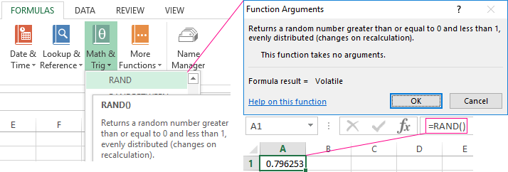
RAND returns an evenly distributed random real number greater than or equal to 0 and less than 1. A new random real number is returned every time the worksheet is calculated.

Syntax

RAND()

The RAND function syntax has no arguments.

Remarks

• To generate a random real number between a and b, use:

=RAND()*(b-a)+a

• If you want to use RAND to generate a random number but don’t want the numbers to change every time the cell is calculated, you can enter =RAND() in the formula bar, and then press F9 to change the formula to a random number. The formula will calculate and leave you with just a value.

Example

Copy the example data in the following table, and paste it in cell A1 of a new Excel worksheet. For formulas to show results, select them, press F2, and then press Enter. You can adjust the column widths to see all the data, if needed.

Formula	Description	Result
=RAND()	A random number greater than or equal to 0 and less than 1	varies
=RAND()*100	A random number greater than or equal to 0 and less than 100	varies
=INT(RAND()*100)	A random whole number greater than or equal to 0 and less than 100	varies
	Note: When a worksheet is recalculated by entering a formula or data in a different cell, or by manually recalculating (press F9), a new random number is generated for any formula that uses the RAND function.

Need more help?

You can always ask an expert in the Excel Tech Community or get support in the Answers community.

See Also

Mersenne Twister algorithm

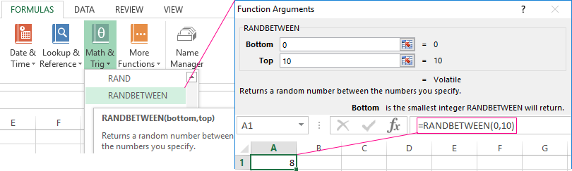
RANDBETWEEN function

Ф

ункция

СЛУЧМЕЖДУ(

)

, английский вариант RANDBETWEEN(),

возвращает случайное ЦЕЛОЕ число в заданном интервале.

Синтаксис функции

СЛУЧМЕЖДУ(

нижняя_граница;верхняя_граница

)

Нижн_граница

— наименьшее целое число, которое возвращает функция.

Верхн_граница

— наибольшее целое число, которое возвращает функция.

Если значение

нижняя_граница

больше значения

верхняя_граница

, функция вернет ошибку #ЧИСЛО! Предполагается, что границы диапазона – целые числа. Если введено число с дробной частью, то дробная часть будет отброшена.

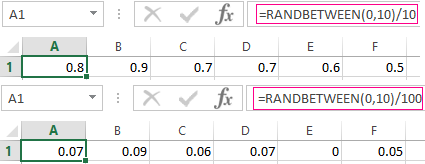
Если необходимо получить случайное число, например, в интервале от 0 до 0,1, то нужно написать следующую формулу:

=СЛУЧМЕЖДУ(0;10)/100

(с точностью 0,01, т.е. случайные значения будут 0,02; 0,05 и т.д.)

=СЛУЧМЕЖДУ(0;1000)/10000

(с точностью 0,0001, т.е. случайные значения будут 0,0689; 0,0254 и т.д.)

Если необходимо получить не целое, а вещественное число, например, в интервале от 3 до 10, то нужно использовать функцию

СЛЧИС()

:

=СЛЧИС()*(10-3)+3

(точностью 15 знаков, т.е. случайные значения будут 7,68866700270417; 8,68428856478223 и т.д.)

Если требуется сгенерировать случайное число от -2,699 до 30,02, причем оно должно быть округлено до тысячных (количество знаков после запятой случайного числа = максимальному количеству знаков после запятой границ интервала), то сначала нужно определить количество знаков после запятой у обоих границ (см.

файл примера

). Это можно сделать с помощью формулы =

ДЛСТР(A15)-1-ДЛСТР(ЦЕЛОЕ(A15))

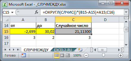
Затем воспользоваться функцией

СЛЧИС()

, округлив значение.

Примечание

. Границы интервала должны быть заданы константой. В случае расчетных значений интервалов результат непредсказуем (см.

Проблемы округления в MS EXCEL

). Совет: Если границы интервала рассчитываются формулами, что в них можно задать необходимую точность.

Функция пересчитывает свое значение после каждого ввода нового значения в любую ячейку листа (или изменения значения ячейки) или нажатии

клавиши

F9

.

We have got a sequence of numbers consisting of virtually independent elements that obey a certain counting distribution. As a rule, it’s a uniform distribution.

There are different ways to generate random numbers in Excel. Let’s view the best of them.



Random Number Function In Excel

1. The function RAND() returns a random real number of a uniform distribution. It will be less than 1, and greater than or equal to 0.
2. The function RANDBETWEEN returns a random integer number.

Let’s view some examples of their practical application.

Selection of random numbers using RAND

This function doesn’t require arguments.

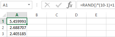
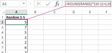
For example, to generate a random real number in the range 1 to 10, use the following formula: =RAND()*(5-1)+1.

The returned random number is distributed uniformly on the interval [1,10].

Each time the sheet is calculated or the value is changed in any cell within the sheet, a new random number is returned. If you want to save the generated set of numbers, replace the formula with its value.

1. Click on the cell containing the random number.
2. Select the formula in the formula bar.
3. Press F9. Then Enter.

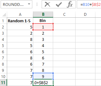
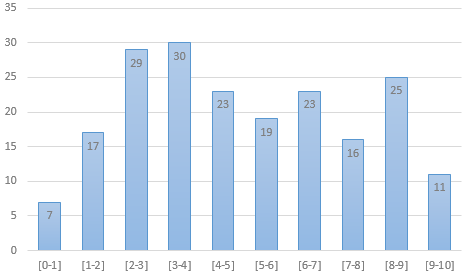
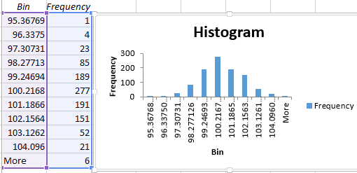
Let us check the uniformity of distribution of the random numbers from the first selection using a distribution bar chart.

1. We round the values that the function =RAND() returns. To do this, we use the function: =ROUND().And fill this formula with the big range: A2:A201.



2. Form the ranges to contain the values (bin). The first such range is 0-0.1. For the subsequent ones use the formula =B2+$B$2.



3. Determine the frequency of random numbers in range A2:A201. In cell C2 use the array formula:

   After input formula, select range C2:C11, press key F2 and press hot keys: CTRL+SHIFT+ENTER. We will execute the formula in the array Excel.



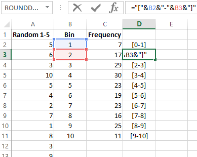
4. Form the ranges with the use of the concatenation character (=»[0,0-«&C2&»]»).



5. Build a distribution bar chart for the 200 values obtained with the use of the RAND() function.

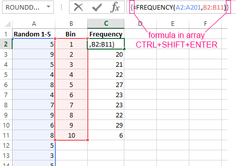
The vertical values represent the frequency. The horizontal ones represent the ranges.



RANDBETWEEN function

The syntax of the RANDBETWEEN function is as follows: (lower limit; upper limit). The first argument must be less than the second. Otherwise, the function will return an error. It is assumed that the limits are integers. The formula discards the fractional part.

An example of the function’s application:

Random numbers with an accuracy of 0.1 and 0.01:

How To Create Random Number Generator In Excel

Let’s create a random number generator that generates values from a certain range. Use a formula of the following form:

The formula randomly selects any of the numbers in the range A1:A10.

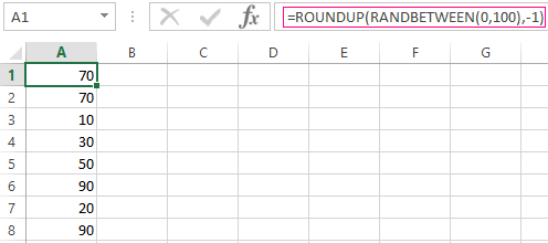
Let’s create a random number generator in the range 0-100, with a step of 10.

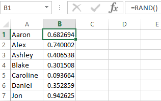
It’s required to select 2 random text values from the list. Using the RAND() function, let’s match the text values in the range A1:A7 with random numbers.

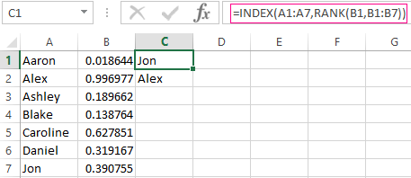
Use the =INDEX function to select two random text values from the initial list.

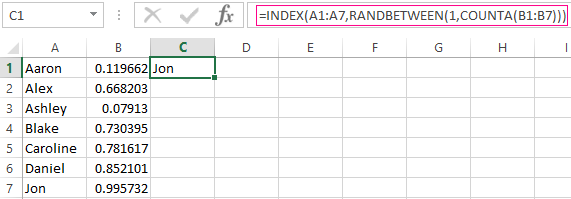
To select one random value from the list, apply the following formula:

Generator Of Standard Distribution Random Numbers

The RAND and RANDBETWEEN functions return random numbers with a single distribution. There’s an equal probability for any value to fall into the lower or upper limit of the requested range. The variation of the target value turns out to be huge.

A standard distribution means most of the generated numbers are close to the target number. Let’s adjust the RANDBETWEEN formula and create an array of data with a standard distribution.

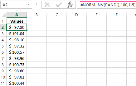
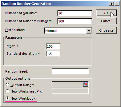
The prime cost of the X product is $100. The entire batch is subject to a standard distribution. The random variable also obeys a standard probability distribution.

Under such conditions, the average value of the range is $100. Let’s generate an array and build a chart that obeys a standard distribution with a standard deviation of $1.5.

Use the function:

Excel calculates the values in the range of probabilities. As the probability of manufacturing a product with a prime cost of $100 is maximal, the formula returns values that are close to 100 more often than other values.

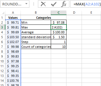
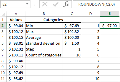
Let’s proceed to building the chart. First of all, you need to create a table containing the categories. To do this, split the array into periods:

1. Determine the minimum and maximum values in the range using the =MIN(A2:102) and =MAX(A2:102) functions.
2. Indicate the value of each period or step. In our example, it’s equal to 1.
3. The number of categories is 10.



4. The lower limit of the table containing the categories is the nearest multiple number rounded down. Enter the formula =ROUNDDOWN(C2,0) into the E1 cell.



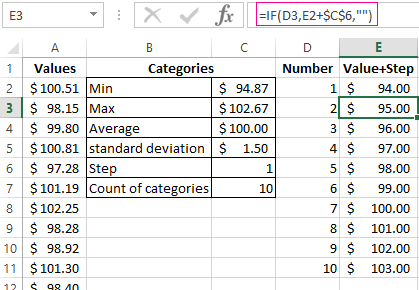
5. In the E2 cell and below, the formula will look as follows:

   That is, each subsequent value is increased by the specified step size.



6. Let’s calculate the number of variables in the given interval. Use the function:

   The formula will look as follows:

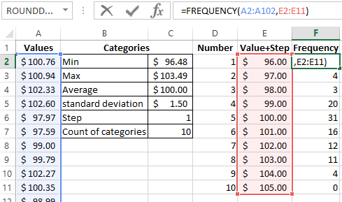
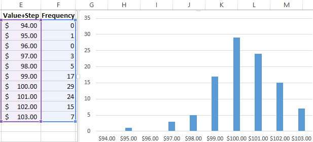
Based on the obtained data, we can build a chart with a normal distribution. The value axis represents the number of variables in the interval; the category axis represents the periods.

A chart with a normal distribution is built. As it should be, its shape resembles a bell.

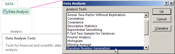
There’s a much simpler way to do the same with the help of the «Data Analysis» package. Select «Random Number Generation».

Click here to learn how to set up the standard feature: «Data Analysis».

Fill in the generation parameters. Set the distribution as «Normal».

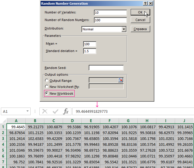
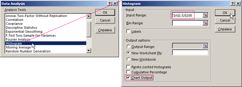
Click OK. It gives us a set of random numbers. Open the «Data Analysis» once again. Select «Histogram». Configure the parameters. Be sure to check the «Chart Output» box.

The obtained result is as follows:

Download random number generators in Excel

An Excel chart with a standard distribution has been built.

Бывают случаи, когда мы хотим смоделировать случайность, фактически не выполняя случайный процесс. Например, предположим, что мы хотим проанализировать конкретный случай 1000000 подбрасываний честной монеты. Мы могли бы подбросить монету миллион раз и записать результаты, но это займет некоторое время. Одна альтернатива – использовать функции случайных чисел в Microsoft Excel. Обе функции RAND и RANDBETWEEN предоставляют способы моделирования случайного поведения.

Функция RAND

Мы начнем с рассмотрения RAND функция. Эта функция используется путем ввода в ячейку Excel следующего текста:

 = RAND () 
 

Функция не принимает аргументов в круглых скобках. Она возвращает случайное действительное число от 0 до 1. Здесь этот интервал действительных чисел считается единым пространством выборки, поэтому при использовании этой функции с равной вероятностью будет возвращено любое число от 0 до 1.

Функцию RAND можно использовать для моделирования случайного процесса. Например, если мы хотим использовать это для имитации подбрасывания монеты, нам нужно будет использовать только функцию ЕСЛИ. Когда наше случайное число меньше 0,5, тогда функция может возвращать H для голов. Когда число больше или равно 0,5, тогда мы могли бы заставить функцию возвращать T для хвостов.

Функция RANDBETWEEN

Вторая функция Excel, работающая со случайностью, называется СЛУЧАЙНОМЕР. Эта функция используется путем ввода следующего текста в пустую ячейку Excel.

 = RANDBETWEEN ([нижняя граница], [верхняя граница]) 
 

Здесь текст в квадратных скобках должен быть заменен двумя разными числами. Функция вернет целое число, которое было случайно выбрано между двумя аргументами функции. Опять же, предполагается единообразное пространство выборки, что означает, что каждое целое число с равной вероятностью будет выбрано.

Например, оценка RANDBETWEEN (1,3) пять раз может привести к 2, 1, 3, 3, 3.

Этот пример показывает важное использование слова «между» в Excel. Это следует интерпретировать в широком смысле, включая верхнюю и нижнюю границы (при условии, что они являются целыми числами).

Опять же, с использованием функции ЕСЛИ мы могли бы очень легко смоделировать подбрасывание любого количества монет. Все, что нам нужно сделать, это использовать функцию RANDBETWEEN (1, 2) вниз по столбцу ячеек. В другом столбце мы могли бы использовать функцию ЕСЛИ, которая возвращает H, если из нашей функции RANDBETWEEN была возвращена 1, и T в противном случае.

Конечно, есть и другие возможности использования функции СЛУЧАЙНА. Это было бы простое приложение для моделирования качения матрицы. Здесь нам понадобится RANDBETWEEN (1, 6). Каждое число от 1 до 6 включительно представляет одну из шести сторон игральной кости..

Предостережения при пересчете

Эти функции, работающие со случайностью, будут возвращать разные значения при каждом пересчете. Это означает, что каждый раз, когда функция оценивается в другой ячейке, случайные числа будут заменяться обновленными случайными числами. По этой причине, если конкретный набор случайных чисел будет изучен позже, было бы целесообразно скопировать эти значения, а затем вставить эти значения в другую часть рабочего листа.

Действительно случайно

Мы должны быть осторожны при использовании этих функций, потому что они являются черными ящиками. Нам неизвестен процесс, который Excel использует для генерации случайных чисел. По этой причине трудно точно знать, что мы получаем случайные числа.