
| title | keywords | f1_keywords | ms.prod | api_name | ms.assetid | ms.date | ms.localizationpriority |
|---|---|---|---|---|---|---|---|
|
Range object (Excel) |
vbaxl10.chm143072 |
vbaxl10.chm143072 |
excel |
Excel.Range |
b8207778-0dcc-4570-1234-f130532cc8cd |
08/14/2019 |
high |
Range object (Excel)
Represents a cell, a row, a column, a selection of cells containing one or more contiguous blocks of cells, or a 3D range.
[!includeAdd-ins note]
Remarks
The default member of Range forwards calls without parameters to the Value property and calls with parameters to the Item member. Accordingly, someRange = someOtherRange is equivalent to someRange.Value = someOtherRange.Value, someRange(1) to someRange.Item(1) and someRange(1,1) to someRange.Item(1,1).
The following properties and methods for returning a Range object are described in the Example section:
- Range and Cells properties of the Worksheet object
- Range and Cells properties of the Range object
- Rows and Columns properties of the Worksheet object
- Rows and Columns properties of the Range object
- Offset property of the Range object
- Union method of the Application object
Example
Use Range (arg), where arg names the range, to return a Range object that represents a single cell or a range of cells. The following example places the value of cell A1 in cell A5.
Worksheets("Sheet1").Range("A5").Value = _
    Worksheets("Sheet1").Range("A1").Value
The following example fills the range A1:H8 with random numbers by setting the formula for each cell in the range. When it’s used without an object qualifier (an object to the left of the period), the Range property returns a range on the active sheet. If the active sheet isn’t a worksheet, the method fails.
Use the Activate method of the Worksheet object to activate a worksheet before you use the Range property without an explicit object qualifier.
Worksheets("Sheet1").Activate
Range("A1:H8").Formula = "=Rand()"    'Range is on the active sheet
The following example clears the contents of the range named Criteria.
[!NOTE]
If you use a text argument for the range address, you must specify the address in A1-style notation (you cannot use R1C1-style notation).
Worksheets(1).Range("Criteria").ClearContents
Use Cells on a worksheet to obtain a range consisting all single cells on the worksheet. You can access single cells via Item(row, column), where row is the row index and column is the column index.
Item can be omitted since the call is forwarded to it by the default member of Range.
The following example sets the value of cell A1 to 24 and of cell B1 to 42 on the first sheet of the active workbook.
Worksheets(1).Cells(1, 1).Value = 24
Worksheets(1).Cells.Item(1, 2).Value = 42
The following example sets the formula for cell A2.
ActiveSheet.Cells(2, 1).Formula = "=Sum(B1:B5)"
Although you can also use Range("A1") to return cell A1, there may be times when the Cells property is more convenient because you can use a variable for the row or column. The following example creates column and row headings on Sheet1. Be aware that after the worksheet has been activated, the Cells property can be used without an explicit sheet declaration (it returns a cell on the active sheet).
[!NOTE]
Although you could use Visual Basic string functions to alter A1-style references, it is easier (and better programming practice) to use theCells(1, 1)notation.
Sub SetUpTable()
Worksheets("Sheet1").Activate
For TheYear = 1 To 5
    Cells(1, TheYear + 1).Value = 1990 + TheYear
Next TheYear
For TheQuarter = 1 To 4
    Cells(TheQuarter + 1, 1).Value = "Q" & TheQuarter
Next TheQuarter
End Sub
Use_expression_.Cells, where expression is an expression that returns a Range object, to obtain a range with the same address consisting of single cells.
On such a range, you access single cells via Item(row, column), where are relative to the upper-left corner of the first area of the range.
Item can be omitted since the call is forwarded to it by the default member of Range.
The following example sets the formula for cell C5 and D5 of the first sheet of the active workbook.
Worksheets(1).Range("C5:C10").Cells(1, 1).Formula = "=Rand()"
Worksheets(1).Range("C5:C10").Cells.Item(1, 2).Formula = "=Rand()"
Use Range (cell1, cell2), where cell1 and cell2 are Range objects that specify the start and end cells, to return a Range object. The following example sets the border line style for cells A1:J10.
[!NOTE]
Be aware that the period in front of each occurrence of the Cells property is required if the result of the preceding With statement is to be applied to the Cells property. In this case, it indicates that the cells are on worksheet one (without the period, the Cells property would return cells on the active sheet).
With Worksheets(1)
    .Range(.Cells(1, 1), _
        .Cells(10, 10)).Borders.LineStyle = xlThick
End With
Use Rows on a worksheet to obtain a range consisting all rows on the worksheet. You can access single rows via Item(row), where row is the row index.
Item can be omitted since the call is forwarded to it by the default member of Range.
[!NOTE]
It’s not legal to provide the second parameter of Item for ranges consisting of rows. You first have to convert it to single cells via Cells.
The following example deletes row 5 and 10 of the first sheet of the active workbook.
Worksheets(1).Rows(10).Delete
Worksheets(1).Rows.Item(5).Delete
Use Columns on a worksheet to obtain a range consisting all columns on the worksheet. You can access single columns via Item(row) [sic], where row is the column index given as a number or as an A1-style column address.
Item can be omitted since the call is forwarded to it by the default member of Range.
[!NOTE]
It’s not legal to provide the second parameter of Item for ranges consisting of columns. You first have to convert it to single cells via Cells.
The following example deletes column «B», «C», «E», and «J» of the first sheet of the active workbook.
Worksheets(1).Columns(10).Delete
Worksheets(1).Columns.Item(5).Delete
Worksheets(1).Columns("C").Delete
Worksheets(1).Columns.Item("B").Delete
Use_expression_.Rows, where expression is an expression that returns a Range object, to obtain a range consisting of the rows in the first area of the range.
You can access single rows via Item(row), where row is the relative row index from the top of the first area of the range.
Item can be omitted since the call is forwarded to it by the default member of Range.
[!NOTE]
It’s not legal to provide the second parameter of Item for ranges consisting of rows. You first have to convert it to single cells via Cells.
The following example deletes the ranges C8:D8 and C6:D6 of the first sheet of the active workbook.
Worksheets(1).Range("C5:D10").Rows(4).Delete
Worksheets(1).Range("C5:D10").Rows.Item(2).Delete
Use_expression_.Columns, where expression is an expression that returns a Range object, to obtain a range consisting of the columns in the first area of the range.
You can access single columns via Item(row) [sic], where row is the relative column index from the left of the first area of the range given as a number or as an A1-style column address.
Item can be omitted since the call is forwarded to it by the default member of Range.
[!NOTE]
It’s not legal to provide the second parameter of Item for ranges consisting of columns. You first have to convert it to single cells via Cells.
The following example deletes the ranges L2:L10, G2:G10, F2:F10 and D2:D10 of the first sheet of the active workbook.
Worksheets(1).Range("C5:Z10").Columns(10).Delete
Worksheets(1).Range("C5:Z10").Columns.Item(5).Delete
Worksheets(1).Range("C5:Z10").Columns("D").Delete
Worksheets(1).Range("C5:Z10").Columns.Item("B").Delete
Use Offset (row, column), where row and column are the row and column offsets, to return a range at a specified offset to another range. The following example selects the cell three rows down from and one column to the right of the cell in the upper-left corner of the current selection. You cannot select a cell that is not on the active sheet, so you must first activate the worksheet.
Worksheets("Sheet1").Activate
  'Can't select unless the sheet is active
Selection.Offset(3, 1).Range("A1").Select
Use Union (range1, range2, …) to return multiple-area ranges—that is, ranges composed of two or more contiguous blocks of cells. The following example creates an object defined as the union of ranges A1:B2 and C3:D4, and then selects the defined range.
Dim r1 As Range, r2 As Range, myMultiAreaRange As Range
Worksheets("sheet1").Activate
Set r1 = Range("A1:B2")
Set r2 = Range("C3:D4")
Set myMultiAreaRange = Union(r1, r2)
myMultiAreaRange.Select
If you work with selections that contain more than one area, the Areas property is useful. It divides a multiple-area selection into individual Range objects and then returns the objects as a collection. Use the Count property on the returned collection to verify a selection that contains more than one area, as shown in the following example.
Sub NoMultiAreaSelection()
    NumberOfSelectedAreas = Selection.Areas.Count
    If NumberOfSelectedAreas > 1 Then
        MsgBox "You cannot carry out this command " & _
            "on multi-area selections"
    End If
End Sub
This example uses the AdvancedFilter method of the Range object to create a list of the unique values, and the number of times those unique values occur, in the range of column A.
Sub Create_Unique_List_Count()
    'Excel workbook, the source and target worksheets, and the source and target ranges.
    Dim wbBook As Workbook
    Dim wsSource As Worksheet
    Dim wsTarget As Worksheet
    Dim rnSource As Range
    Dim rnTarget As Range
    Dim rnUnique As Range
    'Variant to hold the unique data
    Dim vaUnique As Variant
    'Number of unique values in the data
    Dim lnCount As Long

    'Initialize the Excel objects
    Set wbBook = ThisWorkbook
    With wbBook
        Set wsSource = .Worksheets("Sheet1")
        Set wsTarget = .Worksheets("Sheet2")
    End With

    'On the source worksheet, set the range to the data stored in column A
    With wsSource
        Set rnSource = .Range(.Range("A1"), .Range("A100").End(xlDown))
    End With

    'On the target worksheet, set the range as column A.
    Set rnTarget = wsTarget.Range("A1")

    'Use AdvancedFilter to copy the data from the source to the target,
    'while filtering for duplicate values.
    rnSource.AdvancedFilter Action:=xlFilterCopy, _
                            CopyToRange:=rnTarget, _
                            Unique:=True

    'On the target worksheet, set the unique range on Column A, excluding the first cell
    '(which will contain the "List" header for the column).
    With wsTarget
        Set rnUnique = .Range(.Range("A2"), .Range("A100").End(xlUp))
    End With

    'Assign all the values of the Unique range into the Unique variant.
    vaUnique = rnUnique.Value

    'Count the number of occurrences of every unique value in the source data,
    'and list it next to its relevant value.
    For lnCount = 1 To UBound(vaUnique)
        rnUnique(lnCount, 1).Offset(0, 1).Value = _
            Application.Evaluate("COUNTIF(" & _
            rnSource.Address(External:=True) & _
            ",""" & rnUnique(lnCount, 1).Text & """)")
    Next lnCount

    'Label the column of occurrences with "Occurrences"
    With rnTarget.Offset(0, 1)
        .Value = "Occurrences"
        .Font.Bold = True
    End With

End Sub
Methods
- Activate
- AddComment
- AddCommentThreaded
- AdvancedFilter
- AllocateChanges
- ApplyNames
- ApplyOutlineStyles
- AutoComplete
- AutoFill
- AutoFilter
- AutoFit
- AutoOutline
- BorderAround
- Calculate
- CalculateRowMajorOrder
- CheckSpelling
- Clear
- ClearComments
- ClearContents
- ClearFormats
- ClearHyperlinks
- ClearNotes
- ClearOutline
- ColumnDifferences
- Consolidate
- ConvertToLinkedDataType
- Copy
- CopyFromRecordset
- CopyPicture
- CreateNames
- Cut
- DataTypeToText
- DataSeries
- Delete
- DialogBox
- Dirty
- DiscardChanges
- EditionOptions
- ExportAsFixedFormat
- FillDown
- FillLeft
- FillRight
- FillUp
- Find
- FindNext
- FindPrevious
- FlashFill
- FunctionWizard
- Group
- Insert
- InsertIndent
- Justify
- ListNames
- Merge
- NavigateArrow
- NoteText
- Parse
- PasteSpecial
- PrintOut
- PrintPreview
- RemoveDuplicates
- RemoveSubtotal
- Replace
- RowDifferences
- Run
- Select
- SetCellDataTypeFromCell
- SetPhonetic
- Show
- ShowCard
- ShowDependents
- ShowErrors
- ShowPrecedents
- Sort
- SortSpecial
- Speak
- SpecialCells
- SubscribeTo
- Subtotal
- Table
- TextToColumns
- Ungroup
- UnMerge
Properties
- AddIndent
- Address
- AddressLocal
- AllowEdit
- Application
- Areas
- Borders
- Cells
- Characters
- Column
- Columns
- ColumnWidth
- Comment
- CommentThreaded
- Count
- CountLarge
- Creator
- CurrentArray
- CurrentRegion
- Dependents
- DirectDependents
- DirectPrecedents
- DisplayFormat
- End
- EntireColumn
- EntireRow
- Errors
- Font
- FormatConditions
- Formula
- FormulaArray
- FormulaHidden
- FormulaLocal
- FormulaR1C1
- FormulaR1C1Local
- HasArray
- HasFormula
- HasRichDataType
- Height
- Hidden
- HorizontalAlignment
- Hyperlinks
- ID
- IndentLevel
- Interior
- Item
- Left
- LinkedDataTypeState
- ListHeaderRows
- ListObject
- LocationInTable
- Locked
- MDX
- MergeArea
- MergeCells
- Name
- Next
- NumberFormat
- NumberFormatLocal
- Offset
- Orientation
- OutlineLevel
- PageBreak
- Parent
- Phonetic
- Phonetics
- PivotCell
- PivotField
- PivotItem
- PivotTable
- Precedents
- PrefixCharacter
- Previous
- QueryTable
- Range
- ReadingOrder
- Resize
- Row
- RowHeight
- Rows
- ServerActions
- ShowDetail
- ShrinkToFit
- SoundNote
- SparklineGroups
- Style
- Summary
- Text
- Top
- UseStandardHeight
- UseStandardWidth
- Validation
- Value
- Value2
- VerticalAlignment
- Width
- Worksheet
- WrapText
- XPath
See also
- Excel Object Model Reference
[!includeSupport and feedback]
Excel VBA Range Object
Range is a property in VBA that helps specify a particular cell, a range of cells, a row, a column, or a three-dimensional range. In the context of the Excel worksheet, the VBA range object includes a single cell or multiple cells spread across various rows and columns.
For example, the range property in VBA is used to refer to specific rows or columns while writing the code. The code “Range(“A1:A5”).Value=2” returns the number 2 in the range A1:A5.
In VBA, macros are recordedRecording macros is a method whereby excel stores the tasks performed by the user. Every time a macro is run, these exact actions are performed automatically. Macros are created in either the View tab (under the “macros” drop-down) or the Developer tab of Excel.
read more and executed to automate the Excel tasks. This helps perform the repetitive processes in a faster and more accurate way. For running the macros, VBA identifies the cells on which the called tasks are to be performed. It is here that the range object in VBA comes in use.
The VBA range property is similar to the worksheet property and has several applications.
Table of contents
- Excel VBA Range Object
- How to use the VBA Range Function in Excel?
- The Syntax of the VBA Range Property
- Example #1–Select a Single Cell
- Example #2–Select an Entire Row
- Example #3–Select an Entire Column
- Example #4–Select Contiguous Cells
- Example #5–Select Non-contiguous Cells
- Example #6–Select a Range Intersection
- Example #7–Merge a Range of Cells
- Example #8–Clear Formatting of a Range
- Frequently Asked Questions
- Recommended Articles
You are free to use this image on your website, templates, etc, Please provide us with an attribution linkArticle Link to be Hyperlinked
For eg:
Source: VBA Range (wallstreetmojo.com)
How to use the VBA Range Function in Excel?
A hierarchy pattern is used in Excel VBA to refer to the range object. This three-level object hierarchy consists of the following elements:
- Object Qualifier: This refers to the location of the object. It is the workbook or the worksheet where the object is placed.
- Property: This stores the information related to the object.
- Method: This refers to the action that the object will perform. For example, for a given range, the methods are actions like sorting, formatting, selecting, clearing, etc.
The given hierarchical structure is to be followed whenever a VBA objectThe “Object Required” error, also known as Error 424, is a VBA run-time error that occurs when you provide an invalid object, i.e., one that is not available in VBA’s object hierarchy.read more is referred. These three elements are separated by the dot operator (.) in the following way:
Application.Workbooks.Worksheets.Range
Note 1: The range object referred by using the given (three-level) hierarchy is known as a fully qualified reference.
Note 2: The “property” and “method” are used for manipulating cell values.
The Syntax of the VBA Range Property
The syntax of the range property in VBA is shown in the following image:
![]()
For example, to refer to the cell B1 (range) in “sheet3” (worksheet) of “booknew” (workbook), the following reference is used:
Application.Workbooks(“Booknew.xlsm”).Worksheets(“Sheet3”).Range(“B1”)
You can download this VBA Range Excel Template here – VBA Range Excel Template
Example #1–Select a Single Cell
We want to select the cell B2 in “sheet1” of the workbook.
Step 1: Open the workbook saved with the Excel extensionExcel extensions represent the file format. It helps the user to save different types of excel files in various formats. For instance, .xlsx is used for simple data, and XLSM is used to store the VBA code.read more “.xlsm” (macro-enabled workbook). The “.xlsx” format does not allow saving the macros that are presently being written.
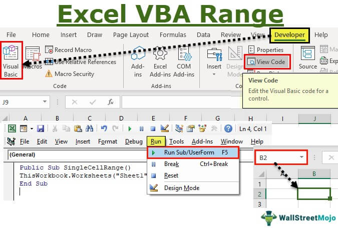
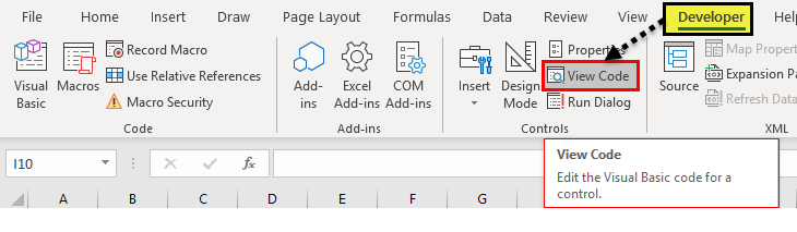
Step 2: Open the VBA editorThe Visual Basic for Applications Editor is a scripting interface. These scripts are primarily responsible for the creation and execution of macros in Microsoft software.read more with the shortcut “ALT+F11.” Alternatively, click “view code” in the “controls” group of the Developer tab, as shown in the following image.
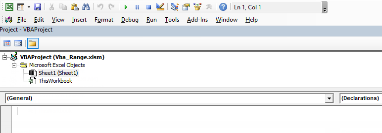
Step 3: The screen, shown in the following image, appears.
Step 4: Enter the following code.
Public Sub SingleCellRange()
ThisWorkbook.Worksheets (“Sheet1”).Range(“B2”).Select
End Sub
With this code, we instruct the program to go to the specified cell (B2) of a particular worksheet and workbook. The action to be performed is to select the given cell.
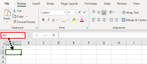
At present, cell A2 is activated, as shown in the following image.
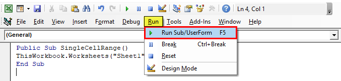
Step 5: Run the code by clicking “run sub/UserForm” from the Run tab. Alternatively, use the Excel shortcut keyAn Excel shortcut is a technique of performing a manual task in a quicker way.read more F5 to run the code.
Step 6: The result is shown in the following image. The cell B2 is selected after the execution of the program. Hence, after running the code, the activated cell is B2.
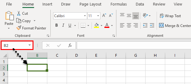
Similarly, the code can be modified to select a variety of cells and ranges and perform different actions on them.
Example #2–Select an Entire Row
We want to select the second row in “sheet1” of the workbook.
Step 1: Enter the following code and run it.
Public Sub EntireRowRange()
ThisWorkbook.Worksheets (“Sheet1”).Range(“2:2”).Select
End Sub
The range (“2:2”) in the code represents the second row.

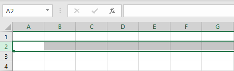
Step 2: The result is shown in the following image. The second row is entirely selected by running the given code.
Example #3–Select an Entire Column
We want to select the column C in “sheet1” of the workbook.
Step 1: Enter the following code and run it.
Public Sub EntireColumnRange()
ThisWorkbook.Worksheets (“Sheet1”).Range(“C:C”).Select
End Sub
The range (“C:C”) in the code represents the column C.

Step 2: The execution of the code and the result is shown in the following image. The column C is entirely selected by running the given code.
Similarly, one can select contiguous and non-contiguous cells, the intersection of cell ranges, etc.
Example #4–Select Contiguous Cells
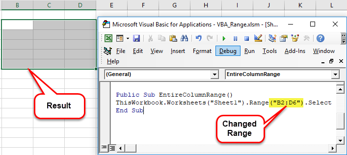
We want to select the range B2:D6 in “sheet1” of the workbook.
Step 1: Enter the following code and run it.
Public Sub EntireColumnRange()
ThisWorkbook.Worksheets (“Sheet1”).Range(“B2:D6”).Select
End Sub
The range (“B2:D6”) in the code represents the contiguous range B2:D6.
Step 2: The result is shown in the following image. The range B2:D6 is selected by running the given code.
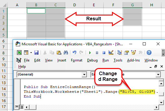
Example #5–Select Non-contiguous Cells
We want to select the ranges B1:C5 and G1:G3 in “sheet1” of the workbook.
Step 1: Enter the following code and run it.
Public Sub EntireColumnRange()
ThisWorkbook.Worksheets (“Sheet1”).Range(“B1:C5, G1:G3”).Select
End Sub
The range (“B1:C5, G1:G3”) in the code represents the two non-contiguous ranges B1:C5 and G1:G3.
Step 2: The result is shown in the following image. The ranges B1:C5 and G1:G3 are selected by running the given code.
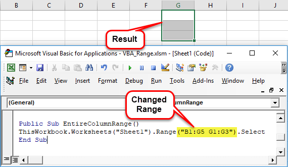
Example #6–Select a Range Intersection
We want to select the intersection of two ranges B1:G5 and G1:G3 in “sheet1” of the workbook.
Step 1: Enter the following code and run it.
Public Sub EntireColumnRange()
ThisWorkbook.Worksheets (“Sheet1”).Range(“B1:G5 G1:G3”).Select
End Sub
The range (“B1:G5 G1:G3”) in the code represents the intersection of the two ranges B1:G5 and G1:G3.
Note: The comma within the two ranges is absent in this case.
Step 2: The result is shown in the following image. The cells common to the ranges B1:G5 and G1:G3 are selected by running the given code. Hence, the common cells in the specified range are G1:G3.
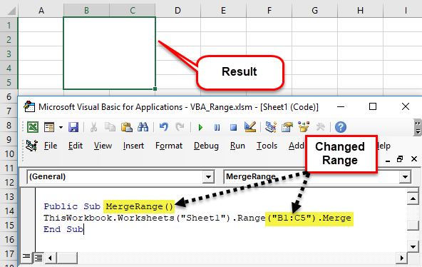
Example #7–Merge a Range of Cells
We want to select and merge the cells B1:C5 in “sheet1” of the workbook.
Step 1: Enter the following code and run it.
Public Sub MergeRange()
ThisWorkbook.Worksheets (“Sheet1”).Range(“B1:C5”).Merge
End Sub
The range (“B1:C5”) represents the range B1:C5 on which we are performing the action “merge.”
Step 2: The result is shown in the following image. The cells in the range B1:C5 have been merged by running the given code.
Example #8–Clear Formatting of a Range
The following image shows the range F2:H6, which is highlighted in yellow. We want to clear the Excel formattingFormatting is a useful feature in Excel that allows you to change the appearance of the data in a worksheet. Formatting can be done in a variety of ways. For example, we can use the styles and format tab on the home tab to change the font of a cell or a table.read more on this range in “sheet1” of the workbook.
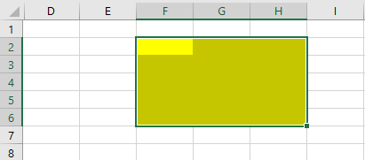
Step 1: Enter the following code and run it.
Public Sub ClearFormats()
ThisWorkbook.Worksheets(“Sheet1”).Range(“F2:H6”).ClearFormats
End Sub
The range (“F2:H6”) in the given syntaxVBA ThisWorkbook refers to the workbook on which the users currently write the code to execute all of the tasks in the current workbook. In this, it doesn’t matter which workbook is active and only requires the reference to the workbook, where the users write the code.read more represents the range F2:H6 from which we are removing the existing formatting.
Step 2: The result is shown in the following image. The formatting from the cells in the range F2:H6 has been cleared by running the given code.
Similarly, the formatting of the entire worksheet can be removed. Moreover, the content of a range of cells can be cleared by using the action “.ClearContents.”
Frequently Asked Questions
1. Define the VBA range.
The VBA range represents a single cell, a row, a column, a group of cells, or a three-dimensional range. The range must be specified in the following hierarchical pattern:
Application.Workbooks.Worksheets.Range
The references following this format are known as fully qualified references. For simplifying these references, the “application” object can be omitted. In such cases, VBA assumes that the user is working on MS Excel.
For example, a simplified reference is Workbooks(“Book2.xlsm”).Worksheets(“Sheet2”).Range
The basic syntax of the VBA range property consists of the keyword “Range” followed by the parentheses. The relevant range is included within double quotation marks.
For example, the following reference refers to cell C1 in the given worksheet and workbook.
Application.Workbooks(“Book2.xlsm”).Worksheets(“Sheet2”).Range(“C1”)
2. How to copy and paste the VBA range?
The following syntax helps copy the range C1:C5:
Range(“C1:C5”).Copy
The following syntax helps copy the range C1:C5 from the present sheet to “sheet3”:
Range(“C1:C5”).Copy destination:= Worksheets(“Sheet3”).Range(“D1”)
The following syntax helps paste in cell D1 of “sheet3”:
Worksheets(“Sheet3”).Range(“D1”).PasteSpecial
Note: Alternatively, the range can be first selected and the resulting selection can be copied.
3. How to clear cells in a VBA range?
The following syntax helps clear the values, comments, and formats from the range C1:C5:
Range(“C1:C5”).Clear
The following syntax helps clear the content or values from the range C1:C5:
Range(“C1:C5”).ClearContents
Note: The clearing methods “ClearNotes,” “ClearComments,” “ClearOutline,” “ClearHyperlinks,” and so on clear particular types of data from the range.
Recommended Articles
This has been a guide to VBA Range. Here we learn how to select a particular cell and range of cells with the help of VBA range objects and examples in Excel. You may also have a look at other articles related to Excel VBA –
- VBA Application.Match
- Excel VBA Cells Reference
- Use VLookup in VBA
- Using VBA Msg Box
“It is a capital mistake to theorize before one has data”- Sir Arthur Conan Doyle
This post covers everything you need to know about using Cells and Ranges in VBA. You can read it from start to finish as it is laid out in a logical order. If you prefer you can use the table of contents below to go to a section of your choice.
Topics covered include Offset property, reading values between cells, reading values to arrays and formatting cells.
A Quick Guide to Ranges and Cells
| Function | Takes | Returns | Example | Gives |
|---|---|---|---|---|
|
Range |
cell address | multiple cells | .Range(«A1:A4») | $A$1:$A$4 |
| Cells | row, column | one cell | .Cells(1,5) | $E$1 |
| Offset | row, column | multiple cells | Range(«A1:A2») .Offset(1,2) |
$C$2:$C$3 |
| Rows | row(s) | one or more rows | .Rows(4) .Rows(«2:4») |
$4:$4 $2:$4 |
| Columns | column(s) | one or more columns | .Columns(4) .Columns(«B:D») |
$D:$D $B:$D |
Download the Code
The Webinar
If you are a member of the VBA Vault, then click on the image below to access the webinar and the associated source code.
(Note: Website members have access to the full webinar archive.)

Introduction
This is the third post dealing with the three main elements of VBA. These three elements are the Workbooks, Worksheets and Ranges/Cells. Cells are by far the most important part of Excel. Almost everything you do in Excel starts and ends with Cells.
Generally speaking, you do three main things with Cells
- Read from a cell.
- Write to a cell.
- Change the format of a cell.
Excel has a number of methods for accessing cells such as Range, Cells and Offset.These can cause confusion as they do similar things and can lead to confusion
In this post I will tackle each one, explain why you need it and when you should use it.
Let’s start with the simplest method of accessing cells – using the Range property of the worksheet.
Important Notes
I have recently updated this article so that is uses Value2.
You may be wondering what is the difference between Value, Value2 and the default:
' Value2
Range("A1").Value2 = 56

' Value
Range("A1").Value = 56

' Default uses value
Range("A1") = 56
Using Value may truncate number if the cell is formatted as currency. If you don’t use any property then the default is Value.
It is better to use Value2 as it will always return the actual cell value(see this article from Charle Williams.)
The Range Property
The worksheet has a Range property which you can use to access cells in VBA. The Range property takes the same argument that most Excel Worksheet functions take e.g. “A1”, “A3:C6” etc.
The following example shows you how to place a value in a cell using the Range property.
' https://excelmacromastery.com/
Public Sub WriteToCell()

    ' Write number to cell A1 in sheet1 of this workbook
    ThisWorkbook.Worksheets("Sheet1").Range("A1").Value2 = 67

    ' Write text to cell A2 in sheet1 of this workbook
    ThisWorkbook.Worksheets("Sheet1").Range("A2").Value2 = "John Smith"

    ' Write date to cell A3 in sheet1 of this workbook
    ThisWorkbook.Worksheets("Sheet1").Range("A3").Value2 = #11/21/2017#

End Sub
As you can see Range is a member of the worksheet which in turn is a member of the Workbook. This follows the same hierarchy as in Excel so should be easy to understand. To do something with Range you must first specify the workbook and worksheet it belongs to.
For the rest of this post I will use the code name to reference the worksheet.

The following code shows the above example using the code name of the worksheet i.e. Sheet1 instead of ThisWorkbook.Worksheets(“Sheet1”).
' https://excelmacromastery.com/
Public Sub UsingCodeName()

    ' Write number to cell A1 in sheet1 of this workbook
    Sheet1.Range("A1").Value2 = 67

    ' Write text to cell A2 in sheet1 of this workbook
    Sheet1.Range("A2").Value2 = "John Smith"

    ' Write date to cell A3 in sheet1 of this workbook
    Sheet1.Range("A3").Value2 = #11/21/2017#

End Sub
You can also write to multiple cells using the Range property
' https://excelmacromastery.com/
Public Sub WriteToMulti()

    ' Write number to a range of cells
    Sheet1.Range("A1:A10").Value2 = 67

    ' Write text to multiple ranges of cells
    Sheet1.Range("B2:B5,B7:B9").Value2 = "John Smith"

End Sub
You can download working examples of all the code from this post from the top of this article.
The Cells Property of the Worksheet
The worksheet object has another property called Cells which is very similar to range. There are two differences
- Cells returns a range of one cell only.
- Cells takes row and column as arguments.
The example below shows you how to write values to cells using both the Range and Cells property
' https://excelmacromastery.com/
Public Sub UsingCells()

    ' Write to A1
    Sheet1.Range("A1").Value2 = 10
    Sheet1.Cells(1, 1).Value2  = 10

    ' Write to A10
    Sheet1.Range("A10").Value2 = 10
    Sheet1.Cells(10, 1).Value2  = 10

    ' Write to E1
    Sheet1.Range("E1").Value2 = 10
    Sheet1.Cells(1, 5).Value2  = 10

End Sub
You may be wondering when you should use Cells and when you should use Range. Using Range is useful for accessing the same cells each time the Macro runs.
For example, if you were using a Macro to calculate a total and write it to cell A10 every time then Range would be suitable for this task.
Using the Cells property is useful if you are accessing a cell based on a number that may vary. It is easier to explain this with an example.
In the following code, we ask the user to specify the column number. Using Cells gives us the flexibility to use a variable number for the column.
' https://excelmacromastery.com/
Public Sub WriteToColumn()

    Dim UserCol As Integer

    ' Get the column number from the user
    UserCol = Application.InputBox(" Please enter the column...", Type:=1)

    ' Write text to user selected column
    Sheet1.Cells(1, UserCol).Value2 = "John Smith"

End Sub
In the above example, we are using a number for the column rather than a letter.
To use Range here would require us to convert these values to the letter/number cell reference e.g. “C1”. Using the Cells property allows us to provide a row and a column number to access a cell.
Sometimes you may want to return more than one cell using row and column numbers. The next section shows you how to do this.
Using Cells and Range together
As you have seen you can only access one cell using the Cells property. If you want to return a range of cells then you can use Cells with Ranges as follows
' https://excelmacromastery.com/
Public Sub UsingCellsWithRange()

    With Sheet1
        ' Write 5 to Range A1:A10 using Cells property
        .Range(.Cells(1, 1), .Cells(10, 1)).Value2 = 5

        ' Format Range B1:Z1 to be bold
        .Range(.Cells(1, 2), .Cells(1, 26)).Font.Bold = True

    End With

End Sub
As you can see, you provide the start and end cell of the Range. Sometimes it can be tricky to see which range you are dealing with when the value are all numbers. Range has a property called Address which displays the letter/ number cell reference of any range. This can come in very handy when you are debugging or writing code for the first time.
In the following example we print out the address of the ranges we are using:
' https://excelmacromastery.com/
Public Sub ShowRangeAddress()

    ' Note: Using underscore allows you to split up lines of code
    With Sheet1

        ' Write 5 to Range A1:A10 using Cells property
        .Range(.Cells(1, 1), .Cells(10, 1)).Value2 = 5
        Debug.Print "First address is : " _
            + .Range(.Cells(1, 1), .Cells(10, 1)).Address

        ' Format Range B1:Z1 to be bold
        .Range(.Cells(1, 2), .Cells(1, 26)).Font.Bold = True
        Debug.Print "Second address is : " _
            + .Range(.Cells(1, 2), .Cells(1, 26)).Address

    End With

End Sub
In the example I used Debug.Print to print to the Immediate Window. To view this window select View->Immediate Window(or Ctrl G)


You can download all the code for this post from the top of this article.
The Offset Property of Range
Range has a property called Offset. The term Offset refers to a count from the original position. It is used a lot in certain areas of programming. With the Offset property you can get a Range of cells the same size and a certain distance from the current range. The reason this is useful is that sometimes you may want to select a Range based on a certain condition. For example in the screenshot below there is a column for each day of the week. Given the day number(i.e. Monday=1, Tuesday=2 etc.) we need to write the value to the correct column.

We will first attempt to do this without using Offset.
' https://excelmacromastery.com/
' This sub tests with different values
Public Sub TestSelect()

    ' Monday
    SetValueSelect 1, 111.21
    ' Wednesday
    SetValueSelect 3, 456.99
    ' Friday
    SetValueSelect 5, 432.25
    ' Sunday
    SetValueSelect 7, 710.17

End Sub

' Writes the value to a column based on the day
Public Sub SetValueSelect(lDay As Long, lValue As Currency)

    Select Case lDay
        Case 1: Sheet1.Range("H3").Value2 = lValue
        Case 2: Sheet1.Range("I3").Value2 = lValue
        Case 3: Sheet1.Range("J3").Value2 = lValue
        Case 4: Sheet1.Range("K3").Value2 = lValue
        Case 5: Sheet1.Range("L3").Value2 = lValue
        Case 6: Sheet1.Range("M3").Value2 = lValue
        Case 7: Sheet1.Range("N3").Value2 = lValue
    End Select

End Sub
As you can see in the example, we need to add a line for each possible option. This is not an ideal situation. Using the Offset Property provides a much cleaner solution
' https://excelmacromastery.com/
' This sub tests with different values
Public Sub TestOffset()

    DayOffSet 1, 111.01
    DayOffSet 3, 456.99
    DayOffSet 5, 432.25
    DayOffSet 7, 710.17

End Sub

Public Sub DayOffSet(lDay As Long, lValue As Currency)

    ' We use the day value with offset specify the correct column
    Sheet1.Range("G3").Offset(, lDay).Value2 = lValue

End Sub
As you can see this solution is much better. If the number of days in increased then we do not need to add any more code. For Offset to be useful there needs to be some kind of relationship between the positions of the cells. If the Day columns in the above example were random then we could not use Offset. We would have to use the first solution.
One thing to keep in mind is that Offset retains the size of the range. So .Range(“A1:A3”).Offset(1,1) returns the range B2:B4. Below are some more examples of using Offset
' https://excelmacromastery.com/
Public Sub UsingOffset()

    ' Write to B2 - no offset
    Sheet1.Range("B2").Offset().Value2 = "Cell B2"

    ' Write to C2 - 1 column to the right
    Sheet1.Range("B2").Offset(, 1).Value2 = "Cell C2"

    ' Write to B3 - 1 row down
    Sheet1.Range("B2").Offset(1).Value2 = "Cell B3"

    ' Write to C3 - 1 column right and 1 row down
    Sheet1.Range("B2").Offset(1, 1).Value2 = "Cell C3"

    ' Write to A1 - 1 column left and 1 row up
    Sheet1.Range("B2").Offset(-1, -1).Value2 = "Cell A1"

    ' Write to range E3:G13 - 1 column right and 1 row down
    Sheet1.Range("D2:F12").Offset(1, 1).Value2 = "Cells E3:G13"

End Sub
Using the Range CurrentRegion
CurrentRegion returns a range of all the adjacent cells to the given range.
In the screenshot below you can see the two current regions. I have added borders to make the current regions clear.

A row or column of blank cells signifies the end of a current region.
You can manually check the CurrentRegion in Excel by selecting a range and pressing Ctrl + Shift + *.
If we take any range of cells within the border and apply CurrentRegion, we will get back the range of cells in the entire area.
For example
Range(“B3”).CurrentRegion will return the range B3:D14
Range(“D14”).CurrentRegion will return the range B3:D14
Range(“C8:C9”).CurrentRegion will return the range B3:D14
and so on
How to Use
We get the CurrentRegion as follows
' Current region will return B3:D14 from above example
Dim rg As Range
Set rg = Sheet1.Range("B3").CurrentRegion
Read Data Rows Only
Read through the range from the second row i.e.skipping the header row
' Current region will return B3:D14 from above example
Dim rg As Range
Set rg = Sheet1.Range("B3").CurrentRegion

' Start at row 2 - row after header
Dim i As Long
For i = 2 To rg.Rows.Count
    ' current row, column 1 of range
    Debug.Print rg.Cells(i, 1).Value2
Next i
Remove Header
Remove header row(i.e. first row) from the range. For example if range is A1:D4 this will return A2:D4
' Current region will return B3:D14 from above example
Dim rg As Range
Set rg = Sheet1.Range("B3").CurrentRegion

' Remove Header
Set rg = rg.Resize(rg.Rows.Count - 1).Offset(1)

' Start at row 1 as no header row
Dim i As Long
For i = 1 To rg.Rows.Count
    ' current row, column 1 of range
    Debug.Print rg.Cells(i, 1).Value2
Next i
Using Rows and Columns as Ranges
If you want to do something with an entire Row or Column you can use the Rows or Columns property of the Worksheet. They both take one parameter which is the row or column number you wish to access
' https://excelmacromastery.com/
Public Sub UseRowAndColumns()

    ' Set the font size of column B to 9
    Sheet1.Columns(2).Font.Size = 9

    ' Set the width of columns D to F
    Sheet1.Columns("D:F").ColumnWidth = 4

    ' Set the font size of row 5 to 18
    Sheet1.Rows(5).Font.Size = 18

End Sub
Using Range in place of Worksheet
You can also use Cells, Rows and Columns as part of a Range rather than part of a Worksheet. You may have a specific need to do this but otherwise I would avoid the practice. It makes the code more complex. Simple code is your friend. It reduces the possibility of errors.
The code below will set the second column of the range to bold. As the range has only two rows the entire column is considered B1:B2
' https://excelmacromastery.com/
Public Sub UseColumnsInRange()

    ' This will set B1 and B2 to be bold
    Sheet1.Range("A1:C2").Columns(2).Font.Bold = True

End Sub
You can download all the code for this post from the top of this article.
Reading Values from one Cell to another
In most of the examples so far we have written values to a cell. We do this by placing the range on the left of the equals sign and the value to place in the cell on the right. To write data from one cell to another we do the same. The destination range goes on the left and the source range goes on the right.
The following example shows you how to do this:
' https://excelmacromastery.com/
Public Sub ReadValues()

    ' Place value from B1 in A1
    Sheet1.Range("A1").Value2 = Sheet1.Range("B1").Value2

    ' Place value from B3 in sheet2 to cell A1
    Sheet1.Range("A1").Value2 = Sheet2.Range("B3").Value2

    ' Place value from B1 in cells A1 to A5
    Sheet1.Range("A1:A5").Value2 = Sheet1.Range("B1").Value2

    ' You need to use the "Value" property to read multiple cells
    Sheet1.Range("A1:A5").Value2 = Sheet1.Range("B1:B5").Value2

End Sub
As you can see from this example it is not possible to read from multiple cells. If you want to do this you can use the Copy function of Range with the Destination parameter
' https://excelmacromastery.com/
Public Sub CopyValues()

    ' Store the copy range in a variable
    Dim rgCopy As Range
    Set rgCopy = Sheet1.Range("B1:B5")

    ' Use this to copy from more than one cell
    rgCopy.Copy Destination:=Sheet1.Range("A1:A5")

    ' You can paste to multiple destinations
    rgCopy.Copy Destination:=Sheet1.Range("A1:A5,C2:C6")

End Sub
The Copy function copies everything including the format of the cells. It is the same result as manually copying and pasting a selection. You can see more about it in the Copying and Pasting Cells section.
Using the Range.Resize Method
When copying from one range to another using assignment(i.e. the equals sign), the destination range must be the same size as the source range.
Using the Resize function allows us to resize a range to a given number of rows and columns.
For example:
' https://excelmacromastery.com/
Sub ResizeExamples()

    ' Prints A1
    Debug.Print Sheet1.Range("A1").Address

    ' Prints A1:A2
    Debug.Print Sheet1.Range("A1").Resize(2, 1).Address

    ' Prints A1:A5
    Debug.Print Sheet1.Range("A1").Resize(5, 1).Address

    ' Prints A1:D1
    Debug.Print Sheet1.Range("A1").Resize(1, 4).Address

    ' Prints A1:C3
    Debug.Print Sheet1.Range("A1").Resize(3, 3).Address

End Sub
When we want to resize our destination range we can simply use the source range size.
In other words, we use the row and column count of the source range as the parameters for resizing:
' https://excelmacromastery.com/
Sub Resize()

    Dim rgSrc As Range, rgDest As Range

    ' Get all the data in the current region
    Set rgSrc = Sheet1.Range("A1").CurrentRegion

      ' Get the range destination
    Set rgDest = Sheet2.Range("A1")
    Set rgDest = rgDest.Resize(rgSrc.Rows.Count, rgSrc.Columns.Count)

    rgDest.Value2 = rgSrc.Value2

End Sub
We can do the resize in one line if we prefer:
' https://excelmacromastery.com/
Sub ResizeOneLine()

    Dim rgSrc As Range

    ' Get all the data in the current region
    Set rgSrc = Sheet1.Range("A1").CurrentRegion

    With rgSrc
        Sheet2.Range("A1").Resize(.Rows.Count, .Columns.Count).Value2 = .Value2
    End With

End Sub
Reading Values to variables
We looked at how to read from one cell to another. You can also read from a cell to a variable. A variable is used to store values while a Macro is running. You normally do this when you want to manipulate the data before writing it somewhere. The following is a simple example using a variable. As you can see the value of the item to the right of the equals is written to the item to the left of the equals.
' https://excelmacromastery.com/
Public Sub UseVariables()

    ' Create
    Dim number As Long

    ' Read number from cell
    number = Sheet1.Range("A1").Value2

    ' Add 1 to value
    number = number + 1

    ' Write new value to cell
    Sheet1.Range("A2").Value2 = number

End Sub
To read text to a variable you use a variable of type String:
' https://excelmacromastery.com/
Public Sub UseVariableText()

    ' Declare a variable of type string
    Dim text As String

    ' Read value from cell
    text = Sheet1.Range("A1").Value2

    ' Write value to cell
    Sheet1.Range("A2").Value2 = text

End Sub
You can write a variable to a range of cells. You just specify the range on the left and the value will be written to all cells in the range.
' https://excelmacromastery.com/
Public Sub VarToMulti()

    ' Read value from cell
    Sheet1.Range("A1:B10").Value2 = 66

End Sub
You cannot read from multiple cells to a variable. However you can read to an array which is a collection of variables. We will look at doing this in the next section.
How to Copy and Paste Cells
If you want to copy and paste a range of cells then you do not need to select them. This is a common error made by new VBA users.
Note: We normally use Range.Copy when we want to copy formats, formulas, validation. If we want to copy values it is not the most efficient method.
I have written a complete guide to copying data in Excel VBA here.
You can simply copy a range of cells like this:
Range("A1:B4").Copy Destination:=Range("C5")
Using this method copies everything – values, formats, formulas and so on. If you want to copy individual items you can use the PasteSpecial property of range.
It works like this
Range("A1:B4").Copy
Range("F3").PasteSpecial Paste:=xlPasteValues
Range("F3").PasteSpecial Paste:=xlPasteFormats
Range("F3").PasteSpecial Paste:=xlPasteFormulas
The following table shows a full list of all the paste types
| Paste Type |
|---|
| xlPasteAll |
| xlPasteAllExceptBorders |
| xlPasteAllMergingConditionalFormats |
| xlPasteAllUsingSourceTheme |
| xlPasteColumnWidths |
| xlPasteComments |
| xlPasteFormats |
| xlPasteFormulas |
| xlPasteFormulasAndNumberFormats |
| xlPasteValidation |
| xlPasteValues |
| xlPasteValuesAndNumberFormats |
Reading a Range of Cells to an Array
You can also copy values by assigning the value of one range to another.
Range("A3:Z3").Value2 = Range("A1:Z1").Value2
The value of range in this example is considered to be a variant array. What this means is that you can easily read from a range of cells to an array. You can also write from an array to a range of cells. If you are not familiar with arrays you can check them out in this post.
The following code shows an example of using an array with a range:
' https://excelmacromastery.com/
Public Sub ReadToArray()

    ' Create dynamic array
    Dim StudentMarks() As Variant

    ' Read 26 values into array from the first row
    StudentMarks = Range("A1:Z1").Value2

    ' Do something with array here

    ' Write the 26 values to the third row
    Range("A3:Z3").Value2 = StudentMarks

End Sub
Keep in mind that the array created by the read is a 2 dimensional array. This is because a spreadsheet stores values in two dimensions i.e. rows and columns
Going through all the cells in a Range
Sometimes you may want to go through each cell one at a time to check value.
You can do this using a For Each loop shown in the following code
' https://excelmacromastery.com/
Public Sub TraversingCells()

    ' Go through each cells in the range
    Dim rg As Range
    For Each rg In Sheet1.Range("A1:A10,A20")
        ' Print address of cells that are negative
        If rg.Value < 0 Then
            Debug.Print rg.Address + " is negative."
        End If
    Next

End Sub
You can also go through consecutive Cells using the Cells property and a standard For loop.
The standard loop is more flexible about the order you use but it is slower than a For Each loop.
' https://excelmacromastery.com/
Public Sub TraverseCells()

    ' Go through cells from A1 to A10
    Dim i As Long
    For i = 1 To 10
        ' Print address of cells that are negative
        If Range("A" & i).Value < 0 Then
            Debug.Print Range("A" & i).Address + " is negative."
        End If
    Next

    ' Go through cells in reverse i.e. from A10 to A1
    For i = 10 To 1 Step -1
        ' Print address of cells that are negative
        If Range("A" & i) < 0 Then
            Debug.Print Range("A" & i).Address + " is negative."
        End If
    Next

End Sub
Formatting Cells
Sometimes you will need to format the cells the in spreadsheet. This is actually very straightforward. The following example shows you various formatting you can add to any range of cells
' https://excelmacromastery.com/
Public Sub FormattingCells()

    With Sheet1

        ' Format the font
        .Range("A1").Font.Bold = True
        .Range("A1").Font.Underline = True
        .Range("A1").Font.Color = rgbNavy

        ' Set the number format to 2 decimal places
        .Range("B2").NumberFormat = "0.00"
        ' Set the number format to a date
        .Range("C2").NumberFormat = "dd/mm/yyyy"
        ' Set the number format to general
        .Range("C3").NumberFormat = "General"
        ' Set the number format to text
        .Range("C4").NumberFormat = "Text"

        ' Set the fill color of the cell
        .Range("B3").Interior.Color = rgbSandyBrown

        ' Format the borders
        .Range("B4").Borders.LineStyle = xlDash
        .Range("B4").Borders.Color = rgbBlueViolet

    End With

End Sub
Main Points
The following is a summary of the main points
- Range returns a range of cells
- Cells returns one cells only
- You can read from one cell to another
- You can read from a range of cells to another range of cells.
- You can read values from cells to variables and vice versa.
- You can read values from ranges to arrays and vice versa
- You can use a For Each or For loop to run through every cell in a range.
- The properties Rows and Columns allow you to access a range of cells of these types
What’s Next?
Free VBA Tutorial If you are new to VBA or you want to sharpen your existing VBA skills then why not try out the The Ultimate VBA Tutorial.
Related Training: Get full access to the Excel VBA training webinars and all the tutorials.
(NOTE: Planning to build or manage a VBA Application? Learn how to build 10 Excel VBA applications from scratch.)
О чём пойдёт речь?
Знакомство с объектной моделью Excel следует начинать с такого замечательного объекта, как Range. Поскольку любая ячейка — это Range, то без знания, как с этим объектом эффективно взаимодействовать, вам будет затруднительно программировать для Excel. Это очень ладно-скроенный объект. При некоторой сноровке вы найдёте его весьма удобным в эксплуатации.
Что такое объекты?
Мы собираемся изучать объект Range, поэтому пару слов надо сказать, что такое, собственно, «объект«. Всё, что вы наблюдаете в Excel, всё с чем вы работаете — это набор объектов. Например, лист рабочей книги Excel — не что иное, как объект типа WorkSheet. Однотипные объекты объединяют в коллекции себе подобных. Например, листы объединены в коллекцию Sheets. Чтобы не путать друг с другом объекты одного и того же типа, они имеют отличающиеся имена, а также номер индекса в коллекции. Объекты имеют свойства, методы и события.
Свойства — это информация об объекте. Часто эти свойства можно менять, что автоматически влечет изменения внешнего вида объекта или его поведения. Например свойство Visible объекта Worksheet отвечает за видимость листа на экране. Если ему присвоить значение xlSheetHidden (это константа, которая по факту равно нулю), то лист будет скрыт.
Методы — это то, что объект может делать. Например, метод Delete объекта Worksheet удаляет себя из книги. Метод Select делает лист активным.
События — это механизм, при помощи которого вы можете исполнять свой код VBA сразу по факту возникновения того или иного события с вашим объектом. Например, есть возможность выполнять ваш код, как только пользователь сделал текущим определенный лист рабочей книги, либо как только пользователь что-то изменил на этом листе.
Range это диапазон ячеек. Минимум — одна ячейка, максимум — весь лист, теоретически насчитывающий более 17 миллиардов ячеек (строки 2^20 * столбцы 2^14 = 2^34).
В Excel объявлены глобально и всегда готовы к использованию несколько коллекций, имеющий членами объекты типа Range, либо свойства это же типа.
Коллекции глобального объекта Application: Cells, Columns, Rows, а также свойства Range, Selection, ActiveCell, ThisCell.
ActiveCell — активная ячейка текущего листа, ThisCell — если вы написали пользовательскую функцию рабочего листа, то через это свойство вы можете определить какая конкретно ячейка в данный момент пересчитывает вашу функцию. Об остальных перечисленных объектов речь пойдёт ниже.
Работа с отдельными ячейками
| Синтаксическая форма | Комментарии по использованию |
| Range(«D5«) или [D5] |
Ячейка D5 текущего листа. Полная и краткая формы. Тут применим только синтаксис типа A1, но не R1C1. То есть такая конструкция Range(«R1C2«) — вызовет ошибку, даже если в книге Excel включен режим формул R1C1. Разумеется после этой формы вы можете обратиться к свойствам соответствующей ячейки. Например, Range(«D5«).Interior.Color = RGB(0, 255, 0). |
| Cells(5, 4) или Cells(5, «D») | Ячейка D5 текущего листа через свойство Cells. 5 — строка (row), 4 — столбец (column). Допустимость второй формы мало кому известна. |
| Cells(65540) | Ячейку D5 можно адресовать и через указание только одного параметра свойсва Cells. При этом нумерация идёт слева направо, потом сверху вниз. То есть сначала нумеруется вся строка (2^14=16384 колонок) и только потом идёт переход на следующую строку. То есть Cells(16385) вернёт вам ячейку A2, а D5 будет Cells(65540). Пока данный способ выглядит не очень удобным. |
Работа с диапазоном ячеек
| Синтаксическая форма | Комментарии по использованию |
| Range(«A1:B4«) или [A1:B4] | Диапазон ячеек A1:B4 текущего листа. Обратите внимание, что указываются координаты верхнего левого и правого нижнего углов диапазона. Причём первый указываемый угол вполне может быть правым нижним, это не имеет значения. |
| Range(Cells(1, 1), Cells(4, 2)) | Диапазон ячеек A1:B4 текущего листа. Удобно, когда вы знаете именно цифровые координаты углов диапазона. |
Работа со строками
| Синтаксическая форма | Комментарии по использованию |
| Range(«3:5«) или [3:5] | Строки 3, 4 и 5 текущего листа целиком. |
| Range(«A3:XFD3«) или [A3:XFD3] | Строка 3, но с указанием колонок. Просто, чтобы вы понимали, что это тождественные формы. XFD — последняя колонка листа. |
| Rows(«3:3«) | Строка 3 через свойство Rows. Параметр в виде диапазона строк. Двоеточие — это символ диапазона. |
| Rows(3) | Тут параметр — индекс строки в массиве строк. Так можно сослаться только не конкретную строку. Обратите внимание, что в предыдущем примере параметр текстовая строка «3:3» и она взята в кавычки, а тут — чистое число. |
Работа со столбцами
| Синтаксическая форма | Комментарии по использованию |
| Range(«B:B«) или [B:B] | Колонка B текущего листа. |
| Range(«B1:B1048576«) или [B1:B1048576] | То же самое, но с указанием номеров строк, чтобы вы понимали, что это тождественные формы. 2^20=1048576 — максимальный номер строки на листе. |
| Columns(«B:B«) | То же самое через свойство Columns. Параметр — текстовая строка. |
| Columns(2) | То же самое. Параметр — числовой индекс столбца. «A» -> 1, «B» -> 2, и т.д. |
Весь лист
| Синтаксическая форма | Комментарии по использованию |
| Range(«A1:XFD1048576«) или [A1:XFD1048576] | Диапазон размером во всё адресное пространство листа Excel. Воспринимайте эту таблицу лишь как теорию — так работать с листами вам не придётся — слишком большое количество ячеек. Даже современные компьютеры не смогут помочь Excel быстро работать с такими массивами информации. Тут проблема больше даже в самом приложении. |
| Range(«1:1048576«) или [1:1048576] | То же самое, но через строки. |
| Range(«A:XFD«) или [A:XFD] | Аналогично — через адреса столбцов. |
| Cells | Свойство Cells включает в себя ВСЕ ячейки. |
| Rows | Все строки листа. |
| Columns | Все столбцы листа. |
Следует иметь в виду, что свойства Range, Cells, Columns и Rows имеют как объекты типа Worksheet, так и объекты Range. Соответственно в первом случае эти коллекции будут относиться ко всему листу и отсчитываться будут от A1, а вот в случае конкретного объекта Range эти коллекции будут относиться только к ячейкам этого диапазона и отсчитываться будут от левого верхнего угла диапазона. Например Cells(2,2) указывает на ячейку B2, а Range(«C3:D5»).Cells(2,2) укажет на D4.
Также много путаницы в умы вносит тот факт, что объект Range имеет одноименное свойство range. К примеру, Range(«A100:D500»).Range(«A2») — тут выражение до точки ( Range(«A100:D500») ) является объектом Range, выражение после точки ( Range(«A2») ) — свойство range упомянутого объекта, но возвращает это свойство тоже объект типа Range. Вот такие пироги. Из этого следует, что такая цепочка может иметь и более двух членов. Практического смысла в этом будет не много, но синтаксически это будут совершенно корректно, например, так: Range(«CV100:GR200»).Range(«J10:T20»).Range(«A1:B2») укажет на диапазон DE109:DF110.
Ещё один сюрприз таится в том, что объекты Range имеют свойство по-умолчанию Item( RowIndex [, ColumnIndex] ). По правилам VBA при ссылке на default свойства имя свойства (Item) можно опускать. Кстати говоря, то что вы привыкли видеть в скобках после Cells, есть не что иное, как это дефолтовое свойство Item, а не родные параметры Cells, который их не имеет вовсе. Ну ладно к Cells все привыкли и это никакого отторжения не вызывает, но если вы увидите нечто подобное — Range(«C3:D5»)(2,2), то, скорее всего, будете несколько озадачены, а тем временем — это буквально тоже самое, что и у Cells — всё то же дефолтовое свойство Item. Последняя конструкция ссылается на D4. А вот для Columns и Rows свойство Item может быть только одночленным, например Columns(1) — и к этой форме мы тоже вполне привыкли. Однако конструкции вида Columns(2)(3)(4) могут сильно удивить (столбец 7 будет выделен).
Примеры кода
Скачать
Типовые задачи
-
Перебор ячеек в диапазоне (вариант 1)
В данном примере организован цикл For…Next и доступ к ячейкам осуществляется по их индексу. Вместо parRange(i) мы могли бы написать parRange.Item(i) (выше это объяснялось). Обратите внимание, что мы в этом примере успешно применяем, как вариант с parRange(i,c), так и parRange(i). То есть, если мы применяем одночленную форму свойства Item, то диапазон перебирается по строкам (A1, B1, C1, A2, …), а если двухчленную, то столбец у нас зафиксирован и каждая итерация цикла — на новой строке. Это очень интересный эффект, его можно применять для вытягивания таблиц по вертикали. Но — продолжим!
Количество ячеек в диапазоне получено при помощи свойства .Count. Как .Item, так и .Count — это всё атрибуты коллекций, которые широко применяются в объектой модели MS Office и, в частности, Excel.
Sub Handle_Cells_1(parRange As Range)
  For i = 1 To parRange.Count
    parRange(i, 5) = parRange(i).Address & " = " & parRange(i)
  Next
End Sub
-
Перебор ячеек в диапазоне (вариант 2)
В этом примере мы использовали цикл For each…Next, что выглядит несколько лаконичней. Однако, в некоторых случаях вам может потребоваться переменная i из предыдущего примера, например, для вывода результатов в определенные строки листа, поэтому выбирайте удробную вам форму оператора For. Тут в цикле мы «вытягивали» все ячейки диапазона в текстовую строку, чтобы потом отобразить её через функцию MsgBox.
Sub Handle_Cells_2(parRange As Range)
  For Each c In parRange
    strLine = strLine & c.Address & "=" & c & "; "
  Next
  MsgBox strLine
End Sub
-
Перебор ячеек в диапазоне (вариант 3)
Если необходимо перебирать ячейки в порядке A1, A2, A3, B1, …, а не A1, B1, C1, A2, …, то вы можете это организовать при помощи 2-х циклов For. Обратите внимание, как мы узнали количество столбцов (parRange.Columns.Count) и строк (parRange.Rows.Count) в диапазоне, а также на использование свойства Cells. Тут Cells относится к листу и никак не связано с диапазоном parRange.
Sub Handle_Cells_3(parRange As Range)
  colNum = parRange.Columns.Count
  For i = 1 To parRange.Rows.Count
    For j = 1 To colNum
      Cells(i + (j - 1) * colNum, colNum + 2) = parRange(i, j)
    Next j
  Next i
End Sub
-
Перебор строк диапазона
В цикле For each…Next перебираем коллекцию Rows объекта parRange. Для каждой строки формируем цвет на основе первых трёх ячеек каждой строки. Поскульку у нас в ячейках формула, присваивающая ячейке случайное число от 1 до 255, то цвета получаются всегда разные. Оператор With позволяет нам сократить код и, к примеру, вместо Line.Cells(2) написать просто .Cells(2).
Sub Handle_Rows_1(parRange As Range)
  For Each Line In parRange.Rows
    With Line
      .Interior.Color = RGB(.Cells(1), .Cells(2), .Cells(3))
    End With
  Next
End Sub
-
Перебор столбцов
Перебираем коллекцию Columns. Тоже используем оператор With. В последней ячейке каждого столбца у нас хранится размер шрифта для всей колонки, который мы и применяем к свойству Line.Font.Size.
Sub Handle_Columns_1(parRange As Range)
  For Each Line In parRange.Columns
    With Line
      .Font.Size = .Cells(.Cells.Count)
    End With
  Next
End Sub
-
Перебор областей диапазона
Как вы знаете, в Excel можно выделить несвязанные диапазоны и проделать с ними какие-то операции. Поддерживает это и объект Range. Получить диапазон, состоящий из нескольких областей (area) очень легко — достаточно перечислить через запятую адреса соответствующих диапазонов: Range(«A1:B3, B5:D8, Z1:AA12«).
Вот такой составной диапазон и разбирается процедурой, показанной ниже. Организован цикл по коллекции Areas, настроен оператор with на текущий элемент коллекции, и ниже и правее относительно ячейки J1 мы собираем некоторые сведения о свойствах областей составного диапазона (которые каждый по себе, конечно же, тоже являются объектами типа Range). Для задания смещения от ячейки J1 нами впервые использовано очень полезное свойство Offset. Каждый диапазон получает случайный цвет, плюс мы заносим в таблицу порядковый номер диапазона (i), его адрес (.Address), количество ячеек (.Count) и цвет (.Interior.Color) после того, как он вычислен.Sub Handle_Areas_1(parRange As Range) For i = 1 To parRange.Areas.Count With parRange.Areas(i) Cells(1, 10).Offset(i, 0) = i Cells(1, 10).Offset(i, 1) = .Address Cells(1, 10).Offset(i, 2) = .Count .Interior.Color = RGB(Int(Rnd * 255), Int(Rnd * 255), Int(Rnd * 255)) Cells(1, 10).Offset(i, 3) = .Interior.Color End With Next End Sub
Продолжение следует…
Читайте также:
-
Поиск границ текущей области
-
Массивы в VBA
-
Структуры данных и их эффективность
-
Автоматическое скрытие/показ столбцов и строк
The VBA Range Object
The Excel Range Object is an object in Excel VBA that represents a cell, row, column, a selection of cells or a 3 dimensional range. The Excel Range is also a Worksheet property that returns a subset of its cells.
Worksheet Range
The Range is a Worksheet property which allows you to select any subset of cells, rows, columns etc.
Dim r as Range 'Declared Range variable
Set r = Range("A1") 'Range of A1 cell
Set r = Range("A1:B2") 'Square Range of 4 cells - A1,A2,B1,B2
Set r= Range(Range("A1"), Range ("B1")) 'Range of 2 cells A1 and B1
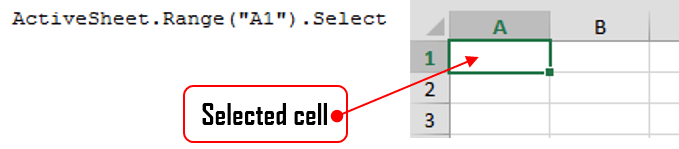
Range("A1:B2").Select 'Select the Cells A1:B2 in your Excel Worksheet
Range("A1:B2").Activate 'Activate the cells and show them on your screen (will switch to Worksheet and/or scroll to this range.
Select a cell or Range of cells using the Select method. It will be visibly marked in Excel:
Working with Range variables
The Range is a separate object variable and can be declared as other variables. As the VBA Range is an object you need to use the Set statement:
Dim myRange as Range
'...
Set myRange = Range("A1") 'Need to use Set to define myRange
The Range object defaults to your ActiveWorksheet. So beware as depending on your ActiveWorksheet the Range object will return values local to your worksheet:
Range("A1").Select
'...is the same as...
ActiveSheet.Range("A1").Select
You might want to define the Worksheet reference by Range if you want your reference values from a specifc Worksheet:
Sheets("Sheet1").Range("A1").Select 'Will always select items from Worksheet named Sheet1
The ActiveWorkbook is not same to ThisWorkbook. Same goes for the ActiveSheet. This may reference a Worksheet from within a Workbook external to the Workbook in which the macro is executed as Active references simply the currently top-most worksheet. Read more here
Range properties
The Range object contains a variety of properties with the main one being it’s Value and an the second one being its Formula.
A Range Value is the evaluated property of a cell or a range of cells. For example a cell with the formula =10+20 has an evaluated value of 20.
A Range Formula is the formula provided in the cell or range of cells. For example a cell with a formula of =10+20 will have the same Formula property.
'Let us assume A1 contains the formula "=10+20"

Debug.Print Range("A1").Value 'Returns: 30

Debug.Print Range("A1").Formula 'Returns: =10+20
Other Range properties include:
Work in progress
Worksheet Cells
A Worksheet Cells property is similar to the Range property but allows you to obtain only a SINGLE CELL, based on its row and column index. Numbering starts at 1:

The Cells property is in fact a Range object not a separate data type.
Excel facilitates a Cells function that allows you to obtain a cell from within the ActiveSheet, current top-most worksheet.
Cells(2,2).Select 'Selects B2
'...is the same as...
ActiveSheet.Cells(2,2).Select 'Select B2
Cells are Ranges which means they are not a separate data type:
Dim myRange as Range
Set myRange = Cells(1,1) 'Cell A1
Range Rows and Columns
As we all know an Excel Worksheet is divided into Rows and Columns. The Excel VBA Range object allows you to select single or multiple rows as well as single or multiple columns. There are a couple of ways to obtain Worksheet rows in VBA:
Getting an entire row or column
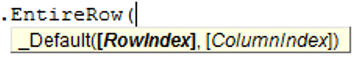
 To get and entire row of a specified Range you need to use the EntireRow property. Although, the function’s parameters suggest taking both a RowIndex and ColumnIndex it is enough just to provide the row number. Row indexing starts at 1.
 To get and entire column of a specified Range you need to use the EntireColumn property. Although, the function’s parameters suggest taking both a RowIndex and ColumnIndex it is enough just to provide the column number. Column indexing starts at 1.
Range("B2").EntireRows(1).Hidden = True 'Gets and hides the entire row 2

Range("B2").EntireColumns(1).Hidden = True 'Gets and hides the entire column 2
The three properties EntireRow/EntireColumn, Rows/Columns and Row/Column are often misunderstood so read through to understand the differences.
Get a row/column of a specified range
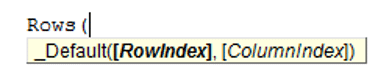 If you want to get a certain row within a Range simply use the Rows property of the Worksheet. Although, the function’s parameters suggest taking both a RowIndex and ColumnIndex it is enough just to provide the row number. Row indexing starts at 1.
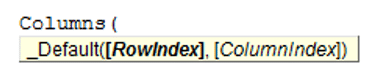 Similarly you can use the Columns function to obtain any single column within a Range. Although, the function’s parameters suggest taking both a RowIndex and ColumnIndex actually the first argument you provide will be the column index. Column indexing starts at 1.
Rows(1).Hidden = True 'Hides the first row in the ActiveSheet
'same as
ActiveSheet.Rows(1).Hidden = True

Columns(1).Hidden = True 'Hides the first column in the ActiveSheet
'same as
ActiveSheet.Columns(1).Hidden = True
To get a range of rows/columns you need to use the Range function like so:
Range(Rows(1), Rows(3)).Hidden = True 'Hides rows 1:3
'same as
Range("1:3").Hidden = True
'same as
ActiveSheet.Range("1:3").Hidden = True

Range(Columns(1), Columns(3)).Hidden = True 'Hides columns A:C
'same as
Range("A:C").Hidden = True
'same as
ActiveSheet.Range("A:C").Hidden = True
Get row/column of specified range
The above approach assumed you want to obtain only rows/columns from the ActiveSheet – the visible and top-most Worksheet. Usually however, you will want to obtain rows or columns of an existing Range. Similarly as with the Worksheet Range property, any Range facilitates the Rows and Columns property.
Dim myRange as Range
Set myRange = Range("A1:C3")

myRange.Rows.Hidden = True 'Hides rows 1:3
myRange.Columns.Hidden = True 'Hides columns A:C

Set myRange = Range("C10:F20")
myRange.Rows(2).Hidden = True 'Hides rows 11
myRange.Columns(3).Hidden = True 'Hides columns E
Getting a Ranges first row/column number
Aside from the Rows and Columns properties Ranges also facilitate a Row and Column property which provide you with the number of the Ranges first row and column.
Set myRange = Range("C10:F20")

'Get first row number
Debug.Print myRange.Row 'Result: 10
'Get first column number
Debug.Print myRange.Column 'Result: 3
Converting Column number to Excel Column
This is an often question that turns up – how to convert a column number to a string e.g. 100 to “CV”.
Function GetExcelColumn(columnNumber As Long)
    Dim div As Long, colName As String, modulo As Long
    div = columnNumber: colName = vbNullString

    Do While div > 0
        modulo = (div - 1) Mod 26
        colName = Chr(65 + modulo) & colName
        div = ((div - modulo) / 26)
    Loop

    GetExcelColumn = colName
End Function
Range Cut/Copy/Paste
Cutting and pasting rows is generally a bad practice which I heavily discourage as this is a practice that is moments can be heavily cpu-intensive and often is unaccounted for.
Copy function
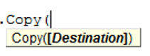 The Copy function works on a single cell, subset of cell or subset of rows/columns.
'Copy values and formatting from cell A1 to cell D1
Range("A1").Copy Range("D1")

'Copy 3x3 A1:C3 matrix to D1:F3 matrix - dimension must be same
Range("A1:C3").Copy Range("D1:F3")

'Copy rows 1:3 to rows 4:6
Range("A1:A3").EntireRow.Copy Range("A4")

'Copy columns A:C to columns D:F
Range("A1:C1").EntireColumn.Copy Range("D1")
The Copy function can also be executed without an argument. It then copies the Range to the Windows Clipboard for later Pasting.
Cut function
![]() The Cut function, similarly as the Copy function, cuts single cells, ranges of cells or rows/columns.
The Cut function, similarly as the Copy function, cuts single cells, ranges of cells or rows/columns.
'Cut A1 cell and paste it to D1
Range("A1").Cut Range("D1")

'Cut 3x3 A1:C3 matrix and paste it in D1:F3 matrix - dimension must be same
Range("A1:C3").Cut Range("D1:F3")

'Cut rows 1:3 and paste to rows 4:6
Range("A1:A3").EntireRow.Cut Range("A4")

'Cut columns A:C and paste to columns D:F
Range("A1:C1").EntireColumn.Cut Range("D1")
The Cut function can be executed without arguments. It will then cut the contents of the Range and copy it to the Windows Clipboard for pasting.
Cutting cells/rows/columns does not shift any remaining cells/rows/columns but simply leaves the cut out cells empty
PasteSpecial function
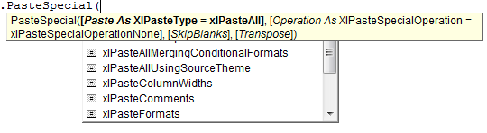 The Range PasteSpecial function works only when preceded with either the Copy or Cut Range functions. It pastes the Range (or other data) within the Clipboard to the Range on which it was executed.
Syntax
The PasteSpecial function has the following syntax:
PasteSpecial( Paste, Operation, SkipBlanks, Transpose)
The PasteSpecial function can only be used in tandem with the Copy function (not Cut)
Parameters
Paste
The part of the Range which is to be pasted. This parameter can have the following values:
| Parameter | Constant | Description | |
|---|---|---|---|
| xlPasteSpecialOperationAdd | 2 | Copied data will be added with the value in the destination cell. | |
| xlPasteSpecialOperationDivide | 5 | Copied data will be divided with the value in the destination cell. | |
| xlPasteSpecialOperationMultiply | 4 | Copied data will be multiplied with the value in the destination cell. | |
| xlPasteSpecialOperationNone | -4142 | No calculation will be done in the paste operation. | |
| xlPasteSpecialOperationSubtract | 3 | Copied data will be subtracted with the value in the destination cell. |
Operation
The paste operation e.g. paste all, only formatting, only values, etc. This can have one of the following values:
| Name | Constant | Description |
|---|---|---|
| xlPasteAll | -4104 | Everything will be pasted. |
| xlPasteAllExceptBorders | 7 | Everything except borders will be pasted. |
| xlPasteAllMergingConditionalFormats | 14 | Everything will be pasted and conditional formats will be merged. |
| xlPasteAllUsingSourceTheme | 13 | Everything will be pasted using the source theme. |
| xlPasteColumnWidths | 8 | Copied column width is pasted. |
| xlPasteComments | -4144 | Comments are pasted. |
| xlPasteFormats | -4122 | Copied source format is pasted. |
| xlPasteFormulas | -4123 | Formulas are pasted. |
| xlPasteFormulasAndNumberFormats | 11 | Formulas and Number formats are pasted. |
| xlPasteValidation | 6 | Validations are pasted. |
| xlPasteValues | -4163 | Values are pasted. |
| xlPasteValuesAndNumberFormats | 12 | Values and Number formats are pasted. |
SkipBlanks
If True then blanks will not be pasted.
Transpose
Transpose the Range before paste (swap rows with columns).
PasteSpecial Examples
'Cut A1 cell and paste its values to D1
Range("A1").Copy
Range("D1").PasteSpecial
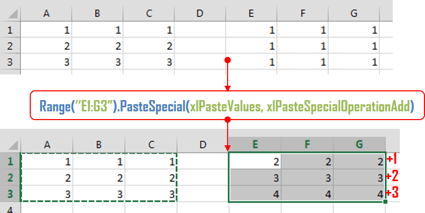
'Copy 3x3 A1:C3 matrix and add all the values to E1:G3 matrix (dimension must be same)
Range("A1:C3").Copy
Range("E1:G3").PasteSpecial xlPasteValues, xlPasteSpecialOperationAdd
Below an example where the Excel Range A1:C3 values are copied an added to the E1:G3 Range. You can also multiply, divide and run other similar operations.
Paste
The Paste function allows you to paste data in the Clipboard to the actively selected Range. Cutting and Pasting can only be accomplished with the Paste function.
'Cut A1 cell and paste its values to D1
Range("A1").Cut
Range("D1").Select
ActiveSheet.Paste

'Cut 3x3 A1:C3 matrix and paste it in D1:F3 matrix - dimension must be same
Range("A1:C3").Cut
Range("D1:F3").Select
ActiveSheet.Paste

'Cut rows 1:3 and paste to rows 4:6
Range("A1:A3").EntireRow.Cut
Range("A4").Select
ActiveSheet.Paste

'Cut columns A:C and paste to columns D:F
Range("A1:C1").EntireColumn.Cut
Range("D1").Select
ActiveSheet.Paste
Range Clear/Delete
The Clear function
The Clear function clears the entire content and formatting from an Excel Range. It does not, however, shift (delete) the cleared cells.
Range("A1:C3").Clear
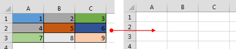
The Delete function
 The Delete function deletes a Range of cells, removing them entirely from the Worksheet, and shifts the remaining Cells in a selected shift direction.
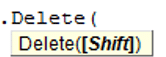
Although the manual Delete cell function provides 4 ways of shifting cells. The VBA Delete Shift values can only be either be xlShiftToLeft or xlShiftUp.
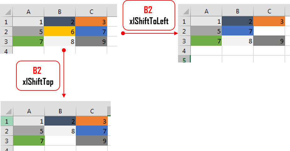
'If Shift omitted, Excel decides - shift up in this case
Range("B2").Delete

'Delete and Shift remaining cells left
Range("B2").Delete xlShiftToLeft

'Delete and Shift remaining cells up
Range("B2").Delete xlShiftTop

'Delete entire row 2 and shift up
Range("B2").EntireRow.Delete

'Delete entire column B and shift left
Range("B2").EntireRow.Delete
Traversing Ranges
Traversing cells is really useful when you want to run an operation on each cell within an Excel Range. Fortunately this is easily achieved in VBA using the For Each or For loops.
Dim cellRange As Range

For Each cellRange In Range("A1:C3")
  Debug.Print cellRange.Value
Next cellRange
Although this may not be obvious, beware of iterating/traversing the Excel Range using a simple For loop. For loops are not efficient on Ranges. Use a For Each loop as shown above. This is because Ranges resemble more Collections than Arrays. Read more on For vs For Each loops here
Traversing the UsedRange
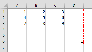 Every Worksheet has a UsedRange. This represents that smallest rectangle Range that contains all cells that have or had at some point values. In other words if the further out in the bottom, right-corner of the Worksheet there is a certain cell (e.g. E8) then the UsedRange will be as large as to include that cell starting at cell A1 (e.g. A1:E8). In Excel you can check the current UsedRange hitting CTRL+END. In VBA you get the UsedRange like this:
ActiveSheet.UsedRange
'same as
UsedRange
You can traverse through the UsedRange like this:
Dim cellRange As Range

For Each cellRange In UsedRange
  Debug.Print "Row: " & cellRange.Row & ", Column: " & cellRange.Column
Next cellRange
The UsedRange is a useful construct responsible often for bloated Excel Workbooks. Often delete unused Rows and Columns that are considered to be within the UsedRange can result in significantly reducing your file size. Read also more on the XSLB file format here
Range Addresses
The Excel Range Address property provides a string value representing the Address of the Range.
![]()
Syntax
Below the syntax of the Excel Range Address property:
Address( [RowAbsolute], [ColumnAbsolute], [ReferenceStyle], [External], [RelativeTo] )
Parameters
RowAbsolute
Optional. If True returns the row part of the reference address as an absolute reference. By default this is True.
$D$10:$G$100 'RowAbsolute is set to True
$D10:$G100 'RowAbsolute is set to False
ColumnAbsolute
Optional. If True returns the column part of the reference as an absolute reference. By default this is True.
$D$10:$G$100 'ColumnAbsolute is set to True
D$10:G$100 'ColumnAbsolute is set to False
ReferenceStyle
Optional. The reference style. The default value is xlA1. Possible values:
| Constant | Value | Description |
|---|---|---|
| xlA1 | 1 | Default. Use xlA1 to return an A1-style reference |
| xlR1C1 | -4150 | Use xlR1C1 to return an R1C1-style reference |
External
Optional. If True then property will return an external reference address, otherwise a local reference address will be returned. By default this is False.
$A$1 'Local
[Book1.xlsb]Sheet1!$A$1 'External
RelativeTo
Provided RowAbsolute and ColumnAbsolute are set to False, and the ReferenceStyle is set to xlR1C1, then you must include a starting point for the relative reference. This must be a Range variable to be set as the reference point.
Merged Ranges
![]() Merged cells are Ranges that consist of 2 or more adjacent cells. To Merge a collection of adjacent cells run Merge function on that Range.
Merged cells are Ranges that consist of 2 or more adjacent cells. To Merge a collection of adjacent cells run Merge function on that Range.
The Merge has only a single parameter – Across, a boolean which if True will merge cells in each row of the specified range as separate merged cells. Otherwise the whole Range will be merged. The default value is False.
Merge examples
To merge the entire Range:
'This will turn of any alerts warning that values may be lost
Application.DisplayAlerts = False

Range("B2:C3").Merge
This will result in the following:
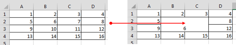
To merge just the rows set Across to True.
'This will turn of any alerts warning that values may be lost
Application.DisplayAlerts = False

Range("B2:C3").Merge True
This will result in the following:
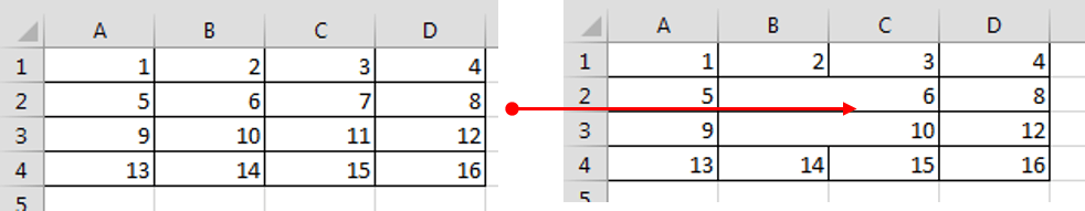
Remember that merged Ranges can only have a single value and formula. Hence, if you merge a group of cells with more than a single value/formula only the first value/formula will be set as the value/formula for your new merged Range
Checking if Range is merged
To check if a certain Range is merged simply use the Excel Range MergeCells property:
Range("B2:C3").Merge

Debug.Print Range("B2").MergeCells 'Result: True
The MergeArea
The MergeArea is a property of an Excel Range that represent the whole merge Range associated with the current Range. Say that $B$2:$C$3 is a merged Range – each cell within that Range (e.g. B2, C3..) will have the exact same MergedArea. See example below:
Range("B2:C3").Merge
Debug.Print Range("B2").MergeArea.Address 'Result: $B$2:$C$3
Named Ranges
Named Ranges are Ranges associated with a certain Name (string). In Excel you can find all your Named Ranges by going to Formulas->Name Manager. They are very useful when working on certain values that are used frequently through out your Workbook. Imagine that you are writing a Financial Analysis and want to use a common Discount Rate across all formulas. Just the address of the cell e.g. “A2”, won’t be self-explanatory. Why not use e.g. “DiscountRate” instead? Well you can do just that.
Creating a Named Range
Named Ranges can be created either within the scope of a Workbook or Worksheet:
Dim r as Range
'Within Workbook
Set r = ActiveWorkbook.Names.Add("NewName", Range("A1"))
'Within Worksheet
Set r = ActiveSheet.Names.Add("NewName", Range("A1"))
This gives you flexibility to use similar names across multiple Worksheets or use a single global name across the entire Workbook.
Listing all Named Ranges
You can list all Named Ranges using the Name Excel data type. Names are objects that represent a single NamedRange. See an example below of listing our two newly created NamedRanges:
Call ActiveWorkbook.Names.Add("NewName", Range("A1"))
Call ActiveSheet.Names.Add("NewName", Range("A1"))

Dim n As Name
For Each n In ActiveWorkbook.Names
  Debug.Print "Name: " & n.Name & ", Address: " & _
       n.RefersToRange.Address & ", Value: "; n.RefersToRange.Value
Next n

'Result:
'Name: Sheet1!NewName, Address: $A$1, Value:  1
'Name: NewName, Address: $A$1, Value:  1
SpecialCells
SpecialCells are a very useful Excel Range property, that allows you to select a subset of cells/Ranges within a certain Range.
Syntax
The SpecialCells property has the following syntax:
SpecialCells( Type, [Value] )
Parameters
Type
The type of cells to be returned. Possible values:
| Constant | Value | Description |
|---|---|---|
| xlCellTypeAllFormatConditions | -4172 | Cells of any format |
| xlCellTypeAllValidation | -4174 | Cells having validation criteria |
| xlCellTypeBlanks | 4 | Empty cells |
| xlCellTypeComments | -4144 | Cells containing notes |
| xlCellTypeConstants | 2 | Cells containing constants |
| xlCellTypeFormulas | -4123 | Cells containing formulas |
| xlCellTypeLastCell | 11 | The last cell in the used range |
| xlCellTypeSameFormatConditions | -4173 | Cells having the same format |
| xlCellTypeSameValidation | -4175 | Cells having the same validation criteria |
| xlCellTypeVisible | 12 | All visible cells |
Value
If Type is equal to xlCellTypeConstants or xlCellTypeFormulas this determines the types of cells to return e.g. with errors.
| Constant | Value |
|---|---|
| xlErrors | 16 |
| xlLogical | 4 |
| xlNumbers | 1 |
| xlTextValues | 2 |
SpecialCells examples
Get Excel Range with Constants
This will return only cells with constant cells within the Range C1:C3:
For Each r In Range("A1:C3").SpecialCells(xlCellTypeConstants)
  Debug.Print r.Value
Next r
Search for Excel Range with Errors
For Each r In ActiveSheet.UsedRange.SpecialCells(xlCellTypeFormulas, xlErrors)
  Debug.Print r.Address
Next r
Ranges are a key concept in Excel, and knowing how to work with them is essential for anyone who wants to program or automate their work using Excel VBA.
In this tutorial, we’ll take a look at how to work with Excel ranges in VBA. We’ll start by discussing what a Range object is. Then, we’ll look at the different ways of referencing a range. Lastly, we’ll explore various examples of how to work with ranges using VBA code.
Excel VBA: The Range object
The Excel VBA Range object is used to represent a range in a worksheet. A range can be a cell, a group of cells, or even all the 17,179,869,184 cells in a sheet.
When programming with Excel VBA, the Range object is going to be your best friend. That’s because much of your work will focus on manipulating data within sheets. Understanding how to work with the Range object will make it easier for you to perform various actions on cells, such as changing their values, sorting, or doing a copy-paste.
The following is the Excel object hierarchy:
Application > Workbook > Worksheet > Range
You can see that the Excel VBA Range object is a property of the Worksheet object. This means that you can access a range by specifying the name of the sheet and the cell address you want to work with. When you don’t specify a sheet name, by default Excel will look for the range in the active sheet. For example, if Sheet1 is active, then both of these lines will refer to the same cell range:
Range("A1")
Worksheets("Sheet1").Range("A1")
Let’s have a closer look at how to reference a range in the section below.


Referencing a range of cells in Excel VBA
Referring to a Range object in Excel VBA can be done in several ways. We’ll discuss the basic syntax and some alternatives that you might want to use, depending on your needs.
Excel VBA: Syntax for specifying a cell range
To refer to a range that consists of one cell, for example, cell D5, you can use the syntax below:
Range("D5")
To refer to a range of cells, you have two acceptable syntaxes. For example, A1 through D5 can be specified using any one below:
Range("A1:D5")
Range("A1", "D5")
To refer to a range outside the active sheet, you need to include the worksheet name. Here’s an example:
Worksheets("Sheet1").Range("A1:D5")
To refer to an entire row, for example, Row 5:
Range("5:5")
To refer to an entire column, for example, Column D:
Range("D:D")
Excel VBA also allows you to refer to multiple ranges at once by using a comma to separate each area. For example, see the below syntax used for referring to all ranges shown in the image:
Range("B2:D8, F4:G5")
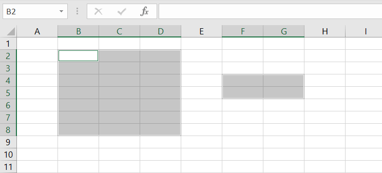
Tip: Notice that all of the syntaxes above use double quotes to enclose the range address. To make it quicker for you to type, you can use shortcuts that involve using square brackets without quotes, as shown in the table below:
| Syntax | Shortcut |
|---|---|
Range("D5") |
[D5] |
Range("A1:D5") |
[A1:D5] |
Range("5:5") |
[5:5] |
Range("B2:D8, F4:G5") |
[B2:D8, F4:G5] |
Excel VBA: Referencing a named range
You have probably already used named ranges in your worksheets. They can be found under Name Manager in the Formulas tab.
To refer to a range named MyRange, use the following code:
Range("MyRange")
Remember to enclose the range’s name in double quotes. Otherwise, Excel thinks that you’re referring to a variable.
Alternatively, you can also use the shortcut syntax discussed previously. In this case, double quotes aren’t used:
[MyRange]
Excel VBA: Referencing a range using the Cells property
Another way to refer to a range is by using the Cells property. This property takes two arguments:
Cells(Row, Column)
You must use a numeric value for Row, but you may use either a numeric or string value for Column. Both of these lines refer to cell D5:
Cells(5, "D")
Cells(5, 4)
The advantage of using the Cells property to refer to ranges becomes clear when you need to loop through rows or columns. You can create a more readable piece of code by using variables as the Cells arguments in a looping.
Excel VBA: Referencing a range using the Offset property
The Offset property provides another handy means for referring to ranges. It allows you to refer to a cell based on the location of another cell, such as the active cell.
Like the Cells property, the Offset property has two parameters. The first determines how many rows to offset, while the second represents the number of columns to offset. Here is the syntax:
Range.Offset(RowOffset, ColumnOffset)
For example, the following code refers to cell D5 from cell A1:
Range("A1").Offset(4,3)
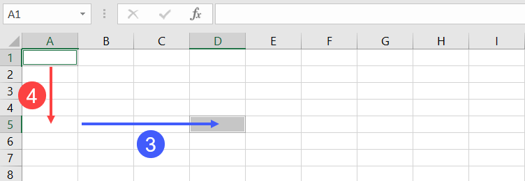
The negative numbers refer to cells that are above or below the range of values. For example, a -2 row offset refers to two rows above the range, and a -1 column offset refers to a column to the left of the range. The following example refers to cell A1:
Range("D3").Offset(-2, -3)
If you need to go over only a row or a column, but not both, you don’t have to enter both the row and the column parameters. You can also use 0 as one or both of the arguments. For example, the following lines refer to D5:
Range("D5").Offset(0, 0)
Range("D2").Offset(3, 0)
Range("G5").Offset(, -3)
Let’s take a look at some of the most common range examples. These examples will show you how to use VBA to select and manipulate ranges in your worksheets. Some of these examples are complete procedures, while others are code snippets that you can just copy-paste to your own Sub to try.
Excel VBA: Select a range of cells
To select a range of cells, use the Select method.
The following line selects a range from A1 to D5 in the active worksheet:
Range("A1:D5").Select
To select a range from A1 to the active cell, use the following line:
Range("A1", ActiveCell).Select
The following code selects from the active cell to 3 rows below the active cell and five columns to the right:
Range(ActiveCell, ActiveCell.Offset(3, 5)).Select
It’s important to note that when you need to select a range on a specific worksheet, you need to ensure that the correct worksheet is active. Otherwise, an error will occur. For example, you want to select B2 to J5 on Sheet1. The following code will generate an error if Sheet1 is not active:
Worksheets("Sheet1").Range("B2:J5").Select
Instead, use these two lines of code to make your code work as expected:
Worksheets("Sheet1").Activate
Range("B2:J5").Select
Excel VBA: Set values to a range
The following statement sets a value of 100 into cell C7 of the active worksheet:
Range("C7").Value = 100
The Value property allows you to represent the value of any cell in a worksheet. It’s a read/write property, so you can use it for both reading and changing values.
You can also set values of a range of any size. The following statement enters the text “Hello” into each cell in the range A1:C7 in Sheet2:
Worksheets("Sheet2").Range("A1:C7").Value = "Hello"
Value is the default property for a Range object. This means that if you don’t provide any properties in your range, Excel will use this Value property.
Both of the following lines enter a value of 100 into cell C7 of the active worksheet:
Range("C7").Value = 100
Range("C7") = 100
Excel VBA: Copy range to another sheet
To copy and paste a range in Excel VBA, you use the Copy and Paste methods. The Copy method copies a range, and the Paste method pastes it into a worksheet. It might look a bit complicated but let’s see what each does with an example below.
Let’s say you have Orders data, as shown in the below screenshot, which is imported from Airtable every day using Coupler.io. This tool allows users to do it automatically on the schedule they want with just a few clicks and no coding required.

In addition, they can combine data from other different sources (such as Jira, Mailchimp, etc.) into one destination for analysis purposes.

As you can see, the data starts from B2. You want to copy only range B2:C11 and paste them to Sheet2 at the same address. The following is an example Sub you can use:
Sub CopyRangeToAnotherSheet()
    Sheets("Sheet1").Activate
    Range("B2:C11").Select
    Selection.Copy

    Sheets("Sheet2").Activate
    Range("B2").Select
    ActiveSheet.Paste
End Sub
Alternatively, you can also use a single line of code as shown below:
Sub CopyRangeToAnotherSheet2()
    Worksheets("Sheet1").Range("B2:C11").Copy Worksheets("Sheet2").Range("B2")
End Sub
The above Sub procedure takes advantage of the fact that the Copy method can use an argument that corresponds to the destination range for the copy operation. Notice that actually, you don’t have to select a range before doing something with it.
Excel VBA: Dynamic range example
In many cases, you may need to copy a range of cells but don’t know exactly how many rows and columns it has. For example, if you use Coupler.io or other integration tools to import data from an external app into Excel on a daily schedule, the number of rows may change over time.
How can you determine this dynamic range? One solution is to use the CurrentRegion property. This property returns an Excel VBA Range object within its boundaries. As long as the data is surrounded by one empty row and one empty column, you can select it with CurrentRegion.
The following line selects the contiguous range around Cell B2:
Range("B2").CurrentRegion.Select

Now, let’s say you want to select only Columns B and C of the range, and from the second row, you can use the following line:
Range("B2", Range("C2").End(xlDown)).Select
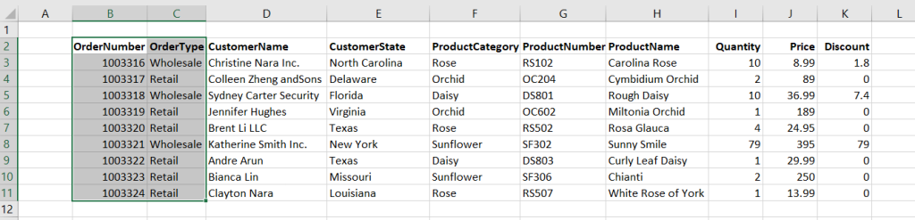
You can now do whatever you want with your selected range — copy or move it to another sheet, format it, and so on.
If you want to find the last row of a used range using Excel VBA, it’s also possible without selecting anything. Here’s the line you can use to find the row number of Column B’s last row data:
' Find the row number of Column B's last row data
RowNumOfLastRow = Cells(Rows.Count, 2).End(xlUp).Row


' Result: 11
MsgBox RowNumOfLastRow
Excel VBA: Loop for each cell in a range
For looping each cell in a range, the For Each loop is an excellent choice. This type of loop is great for looping through a collection of objects such as cells in a range, worksheets in a workbook, or other collections.
The following procedure shows how to loop through each cell in Range B2:K11. We use an object variable named Obj, which refers to the cell being processed. Within the loop, the code checks if the cell contains a formula and then sets its color to blue.
Sub LoopForEachCell()
    Dim obj As Range
    For Each obj In Range("B2:K11")
        If obj.HasFormula Then obj.Font.Color = vbBlue
    Next obj
End Sub
Excel VBA: Loop for each row in a range
When looping through rows (or columns), you can use the Cells property to refer to a range of cells. This makes your code more readable compared to when you’re using the Range syntax.
For example, to loop for each row in range B2:K11 and bold all the cells from Column I to K, you might write a loop like this:
Sub LoopForEachRow()
    For i = 1 To 11
        Range("I" & i & ":K" & i).Font.Bold = True
    Next i
End Sub
Instead of typing in a range address, you can use the Cells property to make the loop easier to read and write. For example, the code below uses the Cells and Resize properties to find the required cell based on the active cell:
Sub LoopForEachRow2()
    For i = 1 To 11
        Cells(i, "I").Resize(, 3).Font.Bold = True
    Next i
End Sub
Excel VBA: Clear a range
There are three ways to clear a range in Excel VBA.
The first is to use the Clear method, which will clear the entire range, including cell contents and formatting.
The second is to use the ClearContents method, which will clear the contents of the range but leave the formatting intact.
The third is to use the ClearFormats method, which will clear the formatting of the range but leave the contents intact.
For example, to clear a range B1 to M15, you can use one of the following lines of code below, based on your needs:
Range("B1:M15").Clear
Range("B1:M15").ClearContents
Range("B1:M15").ClearFormats
Excel VBA: Delete a range
When deleting a range, it differs from just clearing a range. That’s because Excel shifts the remaining cells around to fill up your deleted range.
The code below deletes Row 5 using the Delete method:
Range("5:5").Delete
To delete a range that is not a complete row or column, you have to provide an argument (such as xlToLeft, xlUp — based on your needs) that indicates how Excel should shift the remaining cells.
For example, the following code deletes cell B2 to M10, then fills the resulting gap by shifting the other cells to the left:
Range("B2:M10").Delete xlToLeft
Excel VBA: Delete rows with a specific condition in a range
You can also use a VBA code to delete rows with a specific condition. For example, let’s try to delete all the rows with a discount of 0 from the below sheet:

Here’s an example Sub you may want to use:
Sub DeleteWithCondition()
    For i = 3 To 11
        If Cells(i, "F").Value = 0 Then
            Cells(i, 1).EntireRow.Delete
        End If
    Next i
End Sub
The above code loops from Row 3 to 11. In each loop, it checks the discount value in Column F and removes the entire row if the value equals 0.
Excel VBA: Find values in a range
With the below data, suppose you want to find if there is an order with OrderNumber equal to 1003320 and output its cell address.
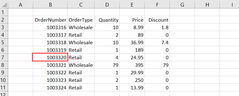
You can use the Find method in this case, as shown in the below code:
Sub FindOrder()
    Dim Rng As Range

    Set Rng = Range("B3:B11").Find("1003320")

    If Rng Is Nothing Then
        MsgBox "The OrderNumber not found."
    Else
        MsgBox Rng.Address
    End If

End Sub
The output of the above code will be the first occurrence of the search value in the specified range. If the value is not found, a message box showing info that the order is not found will appear.
Excel VBA: Add alрhаbеtѕ using Rаngе .Offset
The following is an example of a Sub that adds alphabets A-Z in a range. The code uses Offset to refer to a cell below the active cell in a loop.
Sub AddAlphabetsAZ()
    Dim i As Integer

    ' Use 97 To 122 for lowercase letters
    For i = 65 To 90
        ActiveCell.Value = Chr(i)
        ActiveCell.Offset(1, 0).Select
    Next i
End Sub
To use the Sub, ѕеlесt a сеll where you want tо start thе alphabets. Then, run it by pressing F5. The code will insert A-Z to the cells downward.
Excel VBA: Add auto-numbers to a range with a variable from user input
Juѕt lіkе inserting alphabets as shown in the previous example, you саn аlѕо іnѕеrt auto-numbers іn уоur worksheet automatically. This can be helpful when you work with large data.
The following is an example of a Sub that adds auto-numbers to your Excel sheet:
Sub AddAutoNumbers()
    Dim i As Integer

    On Error GoTo ErrorHandler

    i = InputBox("Enter the maximum number: ", "Enter a value")

    For i = 1 To i
        ActiveCell.Value = i
        ActiveCell.Offset(1, 0).Select
    Next i

ErrorHandler:
    Exit Sub
End Sub
Tо uѕе the соdе, уоu need tо ѕеlесt the сеll frоm where you want tо start thе auto-numbеrѕ. Then, run the Sub. In the message box that appears, enter the maximum value for the auto-numbers and сlісk OK.

Excel VBA: Sum a range
Imagine that you have written a Sub procedure to import Orders.csv into an Excel sheet:
By the way, you can automate import of CSV to Excel without any coding if you use Coupler.io

You want to sum up all the discount values and put the result in J12. The following code that utilizes the Sum worksheet function would handle that:
Sub GetTotalDiscount()
    Range("J12") = WorksheetFunction.Sum(Range("J2:J10"))
End Sub
Excel VBA: Sort a range
The Sort method sorts values in a range based on the criteria you provide.
Suppose you have the following sheet:

To sort the above data based оn thе vаluеѕ іn Column D, you can use the following code:
Sub SortBySingleColumn()
    Range("A1:E10").Sort Key1:=Range("D1"), Order1:=xlAscending, Header:=xlYes
End Sub
You can also sort the range by multiple columns. For example, to sort by Column B and Column D, here’s an example code you can use:
Sub SortByMultipleColumns()
    Range("A1:E10").Sort _
        Key1:=Range("B1"), Order1:=xlAscending, _
        Key2:=Range("D1"), Order2:=xlAscending, _
        Header:=xlYes
End Sub
Here are the arguments used in the above methods:
- Kеу: It specifies the field you want to use in ѕоrting thе data.
- Ordеr: It ѕресіfies whеthеr уоu wаnt tо sort the dаtа іn аѕсеndіng or dеѕсеndіng order.
- Header: It spесіfies whеthеr уоur data hаѕ hеаdеrѕ оr nоt.
Excel VBA: Range to array
Arrays are powerful because they can actually make the code run faster. Especially when working with large data, you can use arrays to make all the processing happen in memory and then write the data to the sheet once.
For example, suppose you have the following sheet:

The following Sub uses a variable X, which is a Variant data type, to store the value of Range A2:E10. Variants can hold any type of data, including arrays.
Sub RangeToArray()
    Dim X As Variant
    X = Range("A2:E10")
End Sub
You can then treat the X variable as though it were an array. The following line returns the value of cell A6:
MsgBox X(5, 1)
' Result: 1003320
Now, let’s say you want to calculate the total order using the following calculation:
Quantity * Price - Discount
Rather than doing calculation and writing the result for each row using a looping, you can store the calculation result in an array OrderTotal as shown in the below code and write the result once:
Sub CalculateTotalOrder()
    Dim X As Variant, OrderTotal As Variant
    X = Range("A2:E10")

    ReDim OrderTotal(UBound(X))

    For i = LBound(X) To UBound(X)
        OrderTotal(i - 1) = X(i, 3) * X(i, 4) - X(i, 5)
    Next i

    Range("F1") = "OrderTotal"

    Range("F2").Resize(UBound(OrderTotal)) = _
        Application.Transpose(OrderTotal)

End Sub
Here’s the final result:
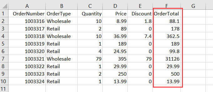
Subscript out of range: Excel VBA Runtime error 9
This error message often happens when you try to access a range of cells in a worksheet that has been deleted or renamed.
Let’s say your code expected a worksheet named Setting. For some reason, this sheet is renamed Settings. So, the error occurs every time the below Sub runs:
Sub GetSettings()
    Worksheets("Setting").Select
    x = Range("A1").Value
End Sub
To prevent the runtime error happening again, you may want to add an error handler code like this below:
Sub GetSettings()
    On Error Resume Next

    ws = Worksheets("Setting")
    Name = ws.Name

    If Not Err.Number = 0 Then
        MsgBox "Expected to find a Setting worksheet, but it is missing."
        Exit Sub
    End If
    On Error GoTo 0

    ws.Select
    x = Range("A1").Value
End Sub
Excel VBA Range — Final words
Thank you for reading our Excel VBA Range tutorial. We hope that you’ve found it helpful! And if there’s anything else about Excel programming or other topics that interest you, be sure to check out our other Excel tutorials.
In addition, you may find that Coupler.io is a valuable tool for you if you’re looking for an easy way to pull and combine your data from multiple sources into one destination for analysis and reporting. This tool also lets you specify the range address of your imported data so you can keep all of your calculations (including. formulas) in the sheets.
Thanks again for reading, and happy coding!
-

Senior analyst programmer

Back to Blog
Focus on your business
goals while we take care of your data!
Try Coupler.io
 What is the first thing that comes to your mind when thinking about Excel?
In my case, it’s probably cells. After all, most of the time we spend working with Excel, we’re working with cells. Therefore, it makes sense that, when using Visual Basic for Applications for purposes of becoming more efficient users of Excel, one of the topics we must learn is how to work with cells within the VBA environment.
This VBA tutorial provides a basic explanation of how to work with cells using Visual Basic for Applications. More precisely, in this particular post I explain all the basic details you need to know to work with Excel’s VBA Range object. Range is the object that you use for purposes of referencing and working with cells within VBA.
However, the importance of Excel’s VBA Range object doesn’t end with the above. A substantial amount of the work you carry out with Excel involves the Range object. The Range object is one of the most commonly used objects in Excel VBA.
Despite the importance of Excel’s VBA Range, creating references to objects is generally one of the most confusing topics for users who are beginning to work with macros and Visual Basic for Applications. In the case of cell ranges, this is (to a certain extent) understandable, since VBA allows you to refer to ranges in many different ways.
The fact remains that, regardless of how confusing the topic of Excel’s VBA Range object may be, you must master it in order to become a macro and VBA expert. My main purpose with this VBA tutorial is to help you understand the basic matters surrounding this topic and illustrate the most common ways in which you can refer to Excel’s VBA Range object using Visual Basic for Applications.
More precisely, in this post you’ll learn about the following topics related to Excel’s VBA Range object:
Let’s start by taking a more detailed look at…
What Is Excel’s VBA Range Object
Excel’s VBA Range is an object. Objects are what is manipulated by Visual Basic for Applications.
More precisely, you can use the Range object to represent a range within a worksheet. This means that, by using Excel’s VBA Range object, you can refer to:
- A single cell.
- A row or a column of cells.
- A selection of cells, regardless of whether they’re contiguous or not.
- A 3-D range.
As you can see from the above, the size of Excel’s VBA Range objects can vary widely. At the most basic level, you can be making reference to a single (1) cell. On the other extreme, you have the possibility of referencing all of the cells in an Excel worksheet.
Despite this flexibility when referring to cells within a particular Excel worksheet, Excel’s VBA Range object does have some limitations. The most relevant is that you can only use it to refer to a single Excel worksheet at a time. Therefore, in order to refer to ranges of cells in different worksheets, you must use separate references for each of the worksheets.
How To Refer To Excel’s VBA Range Object
One of the first things you’ll have to learn in order to master Excel’s VBA Range object is how to refer to it. The following sections explain the most relevant rules you need to know in order to craft appropriate references.
The first few sections cover the most basic way of referring to Excel’s VBA Range object: the Range property. This is also how the macro recorder generally refers to the Range object.
However, further down, you’ll find some additional methods to create object references, such as using the Cells or Offset properties.
These are, however, not the only ways to refer to Excel’s VBA Range objects. There are a few more advanced methods, such as using the Application.Union method, which I don’t cover in this beginners VBA tutorial.
You may be wondering, which way is the best for purposes of referring to Excel’s VBA Range object?
Generally, the best method to use in order to craft a reference to Excel’s VBA Range object depends on the context and your specific needs.
Introduction To Referencing Excel’s VBA Range Object And The Object Qualifier
In order to be able to work appropriately with Range objects, you must understand how to work with the 2 main parts of a reference to Excel’s VBA Range object:
- The object qualifier. This makes reference, more generally, to the general rules to creating object references. I cover this topic thoroughly here.
- The relevant property or method that you’re using for purposes of returning a Range object. This makes reference, more generally, to the specific rules that apply to referring to Excel’s VBA Range object.
This VBA tutorial focuses on the second element above: the main properties you can use in order to refer to Excel’s VBA Range object.
Nonetheless, I explain a few key points regarding object referencing below. If you’re interested in learning more about the general rules that apply to object references, please refer to Excel VBA Object Model And Object References: The Essential Guide, which you can find in the Archives.
Introduction To Fully Qualified VBA Object References
Objects are capable of acting as containers for other objects.
At a basic level, when referencing a particular object, you tell Excel what the object is by referencing all of its parents. In other words, you go through Excel’s VBA object hierarchy.
You move through Excel’s object hierarchy by using the dot(.) operator to connect the objects at each of the different levels.
These types of specific references are known as fully qualified references.
How does a fully qualified reference look in the case of Excel’s VBA Range object?
The object at the top of the Excel VBA object hierarchy is Application. Application itself contains other objects.
Excel’s VBA Range object is contained within the Worksheet object. More precisely:
- The Worksheet object has a Range property (Worksheet.Range).
- The Worksheet.Range property returns a Range object.
The parent object of Worksheets is the Workbook object. Workbooks itself is contained within the Application object.
The hierarchical relationship between these different objects looks as follows:

Therefore, the basic structure you must use to refer to Excel’s VBA Range object is the following:
Application.Workbooks.Worksheets.RangeYou’ll notice that a few things within the basic structure described above are ambiguous. In particular, you’ll notice that this doesn’t specify the particular Excel workbook or worksheet that you’re referring to. In order to do this, you must understand…
How To Refer To An Object From A Collection
Within Visual Basic for Applications, an object collection is a group of related objects.
Both Workbooks and Worksheets, which are used to create a fully qualified reference to Excel’s VBA Range object, are examples of collections. There are 2 basic ways to refer to a particular object within a collection:
- Use the VBA object name. In this case, the syntax is “Collection_name(“Object_name”)”.
- Use an index number instead of the object name. If you choose this option, the basic syntax is “Collection_name(Index_number)”.
Notice how, in the first method you must use quotations (“”) within the parentheses. If you use the second method, you don’t have to surround the Index_number with quotes.
Let’s assume, then, that you want to work with the Worksheet named “Sheet1” within the Workbook “Book1.xlsm”. Depending on which of the 2 methods to refer to an object within a collection you use, the reference looks different.
If you create the reference using the VBA object name, the reference looks as follows:
Application.Workbooks("Book1.xlsm").Worksheets("Sheet1").RangeWhereas if you decide to use an index number, the reference is the following:
Application.Workbooks(1).Worksheets(1).RangeI usually use the first option when working with Visual Basic for Applications. Therefore, this is the method that I use in the examples throughout this VBA tutorial.
Simplifying Fully Qualified Object References
Excel’s VBA object model contains some default objects. These are assumed unless you enter something different.
You can simplify fully qualified object references by relying on these default VBA objects. I don’t generally suggest doing this blindly, as it involves some dangers.
There are 2 main types of default objects that you can use for purposes of simplifying fully qualified object references:
- The Application object.
- The active Workbook and Worksheet objects.
The Application object is always assumed. In other words, Visual Basic for Applications always assumes that you’re working with Excel itself. Therefore, you can simplify your fully qualified object references by omitting the Application. For example, in the cases that I use as an example above, the simplified references are as follows:
Workbooks("Book1.xlsm").Worksheets("Sheet1").Range Workbooks(1).Worksheets(1).RangeAdditionally, VBA assumes that you’re working with the current active workbook and active worksheet. This simplification is trickier than the previous one because it relies on you correctly identifying the active workbook and worksheet. As you’ll imagine, this is slightly more difficult than identifying the Excel application itself 😉 .
However, you can also use these 2 default objects for creating even simpler VBA object references. Continuing with the same examples above, these become:
RangeThis brings us to the end of the introduction to the general rules to creating VBA object references. This summary has explained how to create fully qualified references and simplify them for purposes of creating the object qualifier that you use when crafting references to Excel’s VBA Range object.
The following sections focus on the specific rules that you can apply for purposes of referring to Excel’s VBA Range object. These are the most commonly used properties for returning a Range object.
How To Refer To Excel’s VBA Range Object Using The Range Property
The sections above explain, to a certain extent, the basic rules that you can apply to refer to Excel’s VBA Range object. Let’s start by recalling the 2 methods you can use to create a fully qualified reference if you’re working with the worksheet called “Sheet1” within the workbook named “Book1.xlsm”.
Application.Workbooks("Book1.xlsm").Worksheets("Sheet1").Range Application.Workbooks(1).Worksheets(1).RangeYou need to specify the particular range you want to work with. In other words, just using “Range” as it still appears in the examples above, isn’t enough.
Perhaps the most basic way to refer to Excel’s VBA Range object is by using the Range property. When applied, this property returns a Range object which represents a cell or range of cells.
There are 2 versions of the Range property: the Worksheet.Range property and the Range.Range property. The logic behind both of them is the substantially the same. The main difference is to which object they’re applied:
- In the case of the Worksheet.Range property, the Range property is applied to a worksheet.
- When using the Range.Range property, Range is applied to a range.
In other words, the Range property can be applied to 2 different types of objects:
- Worksheet objects.
- Range objects.
In the sections above, I explain how to create fully qualified object references. You’ve probably noticed that, in all of the examples above, the parent of Excel’s VBA Range object is the Worksheet object. In other words, in these cases, the Range property is applied to a Worksheet object.
However, you can also apply the Range property to a Range object. If you do this, the object returned by the Range property changes.
The reason for this, as explained by Microsoft, is that the Range.Range property acts in relation to the object to which it is applied to. Therefore, if you apply the Range.Range property, the property acts relative to the Range object, not the worksheet.
This means that you can apply the Range.Range property for purposes of referencing a range in relation to another range. I provide examples of how such a reference works below.
Basic Syntax Of The Range Property
The basic syntax that you can use to refer to Excel’s VBA Range object is “expression.Range(“Cell_Range”)”. You’ll notice that this syntax follow the general rules that I explain above for other VBA objects such as Workbooks and Worksheets. In particular, you’ll notice that there are 4 basic elements:
- Element #1: The keyword “Range”.
- Element #2: Parentheses that follow the keyword.
- Element #3: The relevant cell range. I explain different ways in which you can define the range below.
- Element #4: Quotations. The Cell_Range to which you’re making reference is generally within quotations (“”).
In this particular case, “expression” is simply a variable representing a Worksheet object (in the case of the Worksheet.Range property) or a Range object (for the Range.Range object).
Perhaps the most interesting item in the syntax of the Range property is the Cell_Range.
Let’s take a look at some of its characteristics…
In very broad terms, you can usually make reference to Cell_Range in a similar way to the one you use when writing a regular Excel formula. This means using A1-style references. However, there are a few important particularities, which I introduce in this section.
Don’t worry if everything seems a little bit confusing at first. I show some sample references in the following sections in order to make everything clear.
You can use 2 different syntaxes to define the range you want to work with:
Syntax #1: (“Cell1”)
This is the minimum you must include for purposes of defining the relevant cell range. As a general rule, when you use this syntax, the argument (Cell1) must be either of the following:
- A string expressing the cell range address.
- The name of a named cell range.
When naming a range, you can use any of the following 3 operators:
- Colon (:): This is the operator you use to set up arrays. In the context of referring to cell ranges, you can use to refer to entire columns or rows, ranges of contiguous cells or ranges of noncontiguous cells.
- Space ( ): This is the intersection operator. As shown below, you can use the intersection operator for purposes of referring to cells that are common to 2 separate ranges.
- Comma (,): This is the union operator, which you can use to combine several ranges. As shown in the example below, you can use this operator when working with ranges of noncontiguous cells.
Syntax #2: “(Cell1, Cell2)”
If you choose to use this syntax, you’re basically delineating the relevant range by naming the cells in 2 of its corners:
- “Cell1” is the cell in the upper-left corner of the range.
- “Cell2” is the cell in the lower-right corner of the range.
However, this syntax isn’t as restrictive as it may seem at first glance. In this case, arguments can include:
- Range objects;
- Cell range addresses;
- Named cell range names; or
- A combination of the above items.
Let’s take a look at some specific applications of the Range property:
How To Refer To A Single Cell Using The Worksheet.Range Property
If the Excel VBA Range object you want to refer to is a single cell, the syntax is simply “Range(“Cell”)”. For example, if you want to make reference to a single cell, such as A1, type “Range(“A1″)”.

We can take it a step further and create a fully qualified reference for this single cell, assuming that we continue to work with Sheet1 within Book1.xlsm:
Application.Workbooks("Book1.xlsm").Worksheets("Sheet1").Range("A1")You’ve probably noticed something very important:
There is no such thing as a Cell object. Cell is not an object by itself. Cells are contained within the Range object.
Perhaps even more accurately, cells are a property. Properties are the characteristics that you can use to describe an object. I cover the topic of object properties here.
You can actually use this property (Cells) to refer to a range. I explain how you can do this below.
The example above applies the Range property to a Worksheet object. In other words, it is an example of the Worksheet.Range property.
Now let’s take a look at what happens if the Range property is applied to a Range object:
How To Refer To A Single Cell In Relation To Another Range Using The Range.Range Property
Let’s assume, that instead of specifying a fully qualified reference as above, you simply use the Selection object as follows:
Selection.Range("A1")Further, let’s assume that the current selection is the cell range between C3 and D5 (cells C3, C4, C5, D3, D4 and D5) of the active Excel worksheet. This selection is a Range object.
Since the Selection object represents the current selected area in the document, the reference above returns cell C3. It doesn’t return cell A1, as the previous fully qualified reference.
The reason for the different behavior of the 2 sample references above is because the Range property behaves relative to the object to which it is applied. In other words, when the Range property is applied to a Range object, it behaves relative to that Range (more precisely, its upper-left corner). When it is applied to a Worksheet object, it behaves relative to the Worksheet.
Creating references by applying the Range property to a Range object is not very straightforward. I personally find it a little confusing and counterintuitive.
However, the ability to refer to cells in relation to other range has several advantages. This allows you to (for example) refer to a cell without knowing its address beforehand.
Fortunately, there are alternatives for purposes of referring to a particular cell in relation to a range. The main one is the Range.Offset property, which I explain below.
How To Refer To An Entire Column Or Row Using The Worksheet.Range Property
Excel’s VBA Range objects can consist of complete rows or columns. You can refer to an entire row or column as follows:


- Row: “Range(“Row_Number:Row_Number”)”.
- Column: “Range(“Column_Letter:Column_Letter”)”.
For example, if you want to refer to the first row (Row 1) of a particular Excel worksheet, the syntax is “Range(“1:1″)”.

If, on the other hand, you want to refer to the first column (Column A), you type “Range(“A:A”).

Assuming that you’re working with Sheet 1 within Book1.xlsm, the fully qualified references are as follows:
Application.Workbooks("Book1.xlsm").Worksheets("Sheet1").Range("1:1") Application.Workbooks("Book1.xlsm").Worksheets("Sheet1").Range("A:A")How To Refer To A Range Of Contiguous Cells Using The Worksheet.Range Property
You can refer to a range of cells by using the following syntax: “Range(“Cell_Range”). I describe how you can use 2 different syntaxes for purposes of referring to these type of ranges above:
- By identifying the full range.
- By delineating the range, naming the cells in its upper-left and lower-right corners.
Let’s take a look at how both of these look like in practice:
If you want to make reference to a range of cells between cells A1 and B5 (A1, A2, A3, A4, A5, B1, B2, B3, B4 and B5), one appropriate syntax is “Range(“A1:B5″)”. Continuing to work with Sheet1 within Book1.xlsm, the fully qualified reference is as follows:
Application.Workbooks("Book1.xlsm").Worksheets("Sheet1").Range("A1:B5")
However, if you choose to apply the second syntax, where you delineate the relevant range, the appropriate syntax is “Range(“A1”, “B5″)”. In this case, the fully qualified reference looks as follows:
Application.Workbooks("Book1.xlsm").Worksheets("Sheet1").Range("A1", "B5")How To Refer To A Range Of NonContiguous Cells Using The Worksheet.Range Property
The syntax for purposes of referring to a range of noncontiguous cells in Excel is very similar to that used to refer to a range of contiguous cells. You simply separate the different areas by using a comma (,). Therefore, the basic syntax is “Range(“Cell_Range_1,Cell_Range_#,…”)”.
Let’s assume that you want to refer to the following ranges of noncontiguous cells:

- Cells A1 to B5 (A1, A2, A3, A4, A5, B1, B2, B3, B4 and B5).
- Cells D1 to D5 (D1, D2, D3, D4 and D5).
You refer to such range by typing “Range(“A1:B5,D1:D5″)”. In this case, the fully qualified reference looks as follows:
Application.Workbooks("Book1.xlsm").Worksheets("Sheet1").Range("A1:B5,D1:D5")

However, when working with ranges of noncontiguous cells, you may want to process each of the different areas separately. The reason for this is that some methods/properties have issues when working with such noncontiguous cell ranges.
You can handle the separate processing with a loop.
How To Refer To The Intersection Of 2 Ranges Using The Worksheet.Range Property
I describe how, when using the Range property, you can use 3 operators for purposes of identifying the relevant Range above. We’ve already gone through examples that use the colon (:) and comma (,) operators. These were used in the previous sections for purposes of referring to ranges of contiguous or noncontiguous cells.
The third operator, space ( ), is useful when you want to refer to the intersection of 2 ranges. The reason for this is clear:
The space ( ) operator is, precisely, the intersection operator.
Let’s assume that you want to refer to the intersection of the following 2 ranges:

- Cells B1 to B10 (B1, B2, B3, B4, B5, B6, B7, B8, B9 and B10).
- Cells A5 to C5 (A5, B5 and C5).

In this case, the appropriate syntax is “Range(“B1:B10 A5:C5″)”. When working with Sheet1 of Book1.xlsm, a fully qualified reference can be constructed as follows:
Application.Workbooks("Book1.xlsm").Worksheets("Sheet1").Range("B1:B10 A5:C5")Such a reference returns the cells that are common to the 2 ranges. In this particular case, the only cell that is common to both ranges is B5.
How To Refer To A Named VBA Range Using The Worksheet.Range Property
If you’re referring to a VBA Range that has a name, the syntax is very similar to the basic case of referring to a single cell. You simply replace the address that you use to refer to the range with the appropriate name.
For example, if you want to create a reference to a VBA Range named “Excel_Tutorial_Example”, the appropriate syntax is “Range(“Excel_Tutorial_Example”)”. In this case, a fully qualified reference looks as follows:
Application.Workbooks("Book1.xlsm").Worksheets("Sheet1").Range("Excel_Tutorial_Example")
Remember to use quotation marks (“”) around the name of the range. If you don’t use quotes, Visual Basic for Applications interprets it as a variable.
How To Refer To Merged Cells Using The Worksheet.Range Property
In general, working with merged cells isn’t that straightforward. In the case of macros this is no exception. The following are some of the (potential) challenges you may face when working with a range that contains merged cells:


- The macro behaving differently from what you expected.
- Issues with sorting.
I may cover the topic of working with merged cells in future tutorials. For the moment, I explain how to refer to merged cells using the Range property. This should help you avoid some of the most common pitfalls when working with merged cells.
The first thing to consider when referring to merged cells is that you can reference them in either of the following 2 ways:
- By referring to the entire merged cell range.
- By referring only to the upper-left cell of the merged range.
Let’s assume that you’re working on an Excel spreadsheet where the cell range from A1 to C5 is merged. This includes cells A1, A2, A3, A4, A5, B1, B2, B3, B4, B5, C1, C2, C3, C4 and C5. In this case, the appropriate syntax is either of the following:
- If you refer to the entire merged range, “Range(“A1:C5″)”. In this case, the fully qualified reference is “Application.Workbooks(“Book1.xlsm”).Worksheets(“Sheet1”).Range(“A1:C5″)”.
- If you refer only to the upper-left cell of the merged range, “Range(“A1″)”. The fully qualified reference under this method is “Application.Workbooks(“Book1.xlsm”).Worksheets(“Sheet1”).Range(“A1″)”.
In both cases, the result is the same.

You should be particularly careful when trying to assign values to merged cells. Generally, you can only carry this operation by assigning the value to the upper-left cell of the range (cell A1 in the example above). Otherwise, Excel VBA (usually) doesn’t:
- Carry out the value assignment; and
- Return an error.
How To Refer To A VBA Range Object Using Shortcuts For The Range Property
References to Excel’s VBA Range object using the Range property can be made shorter using square brackets ([ ]).
You can use this shortcut as follows:
- Don’t use the keyword “Range”.
- Surround the relevant property arguments with square brackets ([ ]) instead of using parentheses and double quotes (“”).
Let’s take a look at how this looks in practice by applying the shortcut to the different cases and examples shown and explained in the sections above.
Shortcut #1: Referring To A Single Cell
Instead of typing “Range(“Cell”)” as explained above, type “[Cell]”.
For example if you’re making reference to cell A1, use “[A1]”. The fully qualified reference for cell A1 in Sheet1 of Book1.xlsm looks as follows:
Application.Workbooks("Book1.xlsm").Worksheets("Sheet1").[A1]

Shortcut #2: Referring To An Entire Row Or Column
In this case, the usual syntax is either “Range(“Row_Number:Row_Number”)” or “Range(“Column_Letter:Column_Letter”)”. I explain this above.
By applying square brackets, you can shorten the references to the following:

- Row: “[Row_Number:Row_Number]”.
- Column: “[Column_Letter:Column_Letter]”.
For example, if you’re referring to the first row (Row 1) or the first column (Column A) of an Excel worksheet, the syntax is as follows:
And the fully qualified references, assuming you’re working with Sheet1 of Book1.xlsm are the following:
Application.Workbooks("Book1.xlsm").Worksheets("Sheet1").[1:1] Application.Workbooks("Book1.xlsm").Worksheets("Sheet1").[A:A]Shortcut #3: Referring To A Range Of Contiguous Cells
Generally, you refer to a range of cells by using the syntax “Range(“Cell_Range”)”. If you’re identifying the full range by using the colon (:) operator, as I explain above, you usually structure the reference as “Range(“Top_Left_Cell:Right_Bottom_Cell”)”.
You can shorten the reference to a range of contiguous cells by using square brackets as follows: “[Top_Left_Cell:Right_Bottom_Cell]”.
For example in order to refer to a range of cells between cells A1 and B5 (A1, A2, A3, A4, A5, B1, B2, B3, B4 and B5), you can type “[A1:B5]”. Alternatively, if you’re using a fully qualified reference and are working with Sheet1 of Book1.xlsm, the syntax is as follows:
Application.Workbooks("Book1.xlsm").Worksheets("Sheet1").[A1:B5]
Shortcut #4: Referring To A Range Of NonContiguous Cells
This case is fairly similar to the previous one, in which we made reference to a range of contiguous cells. However, in order to separate the different areas, you use the comma (,) operator, as explained previously. In other words, the basic syntax is usually “Range(“Cell_Range_1,Cell_Range_#,…”)”.
When using square brackets, you can simplify the reference above to “[Cell_Range_1,Cell_Range_#,…]”.
If you want to refer to the following ranges of noncontiguous cells:

- Cells A1 to B5 (A1, A2, A3, A4, A5, B1, B2, B3, B4 and B5).
- Cells D1 to D5 (D1, D2, D3, D4 and D5).
The syntax of a reference using square brackets is “[A1:B5,D1:D5]”. The fully qualified reference looks as follows:
Application.Workbooks("Book1.xlsm").Worksheets("Sheet1").[A1:B5,D1:D5]

Shortcut #5: Referring To The Intersection Of 2 Ranges
Generally, the syntax for referring to the intersection of 2 ranges uses the space operator and is “Range(“Cell_Range_1 Cell_Range_2″)”. When using square brackets, this becomes “[Cell_Range_1 Cell_Range_2]”.
Let’s go back to the example I use above and assume that you want to refer to the intersection of the following 2 ranges:

- Cells B1 to B10 (B1, B2, B3, B4, B5, B6, B7, B8, B9 and B10).
- Cells A5 to C5 (A5, B5 and C5).
You can create a reference using square brackets as follows: “[B1:B10 A5:C5]”. When working with Sheet1 of Book1.xlsm, the fully qualified reference is:
Application.Workbooks("Book1.xlsm").Worksheets("Sheet1").[B1:B10 A5:C5]And this returns the only cell common to both ranges: B5.
Shortcut #6: Referring To A Named VBA Range
As explained above, when referring to a VBA Range that has a name, you replace the address of the range with the relevant name. Therefore, the basic syntax is “Range(“Range_Name”)”.
When using square brackets, the logic is the same. Therefore, you can refer to a named range by typing “[Range_Name]”.
For example, when referring to a VBA Range named “Excel_Tutorial_Example”, the reference can be structures as “[Excel_Tutorial_Example]”. When using a fully qualified reference, it looks as follows:
Application.Workbooks("Book1.xlsm").Worksheets("Sheet1").[Excel_Tutorial_Example]
How To Refer To A VBA Range Object Using The Cells Property
There is no Cell object within Visual Basic for Applications. There is a Worksheet.Cells property and a Range.Cells property. You can use the Cells property to return a Range object representing the cells.
The main difference between both Cells properties is in connection with the object to which the property is applied to:


- When using the Worksheet.Cells property, you’re applying the property to a Worksheet object.
- When using the Range.Cells property, that property is applied to a Range object.
This is important because, depending on the context, the properties may return different cells. More precisely, when applying the Cells property to a Range object, you’re referring to a cell in relation to another range.
This probably sounds confusing, I agree. Don’t worry, as the explanation and examples below make this topic clear. The most important thing to remember is that the Cells property allows you to refer to a cell range.
Since the basic logic behind both properties (Worksheet.Cells and Range.Cells) is similar, I cover both at the same time.
There are several ways in which you can use the Cells property to refer to a Range object. I explain the main methods of doing this in the following sections.
Syntax Of The Cells Property
The basic syntax of the Cells property is “expression.Cells(Row_Number, Column_Number)”, where:
- “expression” is a variable representing a VBA object. This VBA object can be either a worksheet (in the case of the Worksheet.Cells property) or a range (for the Range.Cells property).
- “Row_Number” and “Column_Number” are the numbers of both the row and the column.
- Is common to use numbers in both cases.
- When using this syntax, you can also use a letter to refer to the column. In this case, wrap the letter in double quotes (“”). Other than the quotations (“”) (surrounding the letter), you don’t need to use other quotations in the same way as you do when using the Range property.
One of the main differences between the Range and the Cells properties is that the Cells property takes row and column numbers as arguments. You can see this reflected in the syntax described above.
There are additional possible ways to implement the Cells property. However, they’re secondary and I explain them below.
The Range object has a property called the Range.Item property, which I explain below. The reason why you can specify the Row_Number and Column_Number arguments immediately after the Cells keyword is that the Range.Item property is the default property of the Range object. This is the same reason why, as explained above, you can also use a letter wrapped in double quotes (“”) to refer to the column. If you’re interested in understanding the relationship between the Range.Item property and the Cells property, please refer to the relevant section below.
For the moment, let’s go back to some of the VBA Ranges that have appeared in previous examples and see how to refer to them using the Cells property.
How To Refer To A Single Cell Using The Worksheet.Cells Property
The most basic use case of the Cells property is referring to a single cell.
The fact that the Cells property can only be used (usually) for purposes of returning a range of 1 cell is one of the main characteristics that distinguishes the Cells from the Range property.
There is actually a way to use the Cells property for purposes of referring to larger cell ranges. However, this involves combining the Range and Cells properties. I explain this method below.
Referring to a single cell using the Cells property is relatively simple. For example, if you want to refer to cell A1 within Sheet1 of Book1.xlsm, the fully qualified reference is pretty much what you’d expect considering the basic syntax shown in the previous section:
Application.Workbooks("Book1.xlsm").Worksheets("Sheet1").Cells(1, 1)
Application.Workbooks("Book1.xlsm").Worksheets("Sheet1").Cells(1, "A")

There is, however, a second way to create references to a single cell when using the Worksheet.Cells property. Let’s take a look at this…
Alternative Syntax For Referring To A Single Cell Using The Worksheet.Cells Property
The syntax of the Cells property that I describe above is probably the one that you’ll use the most in practice.
The following alternative is substantially the same as the syntax that I have explained above. It also starts with “expression.Cells”. The difference lies in the arguments that appear within the parentheses.
This alternative syntax is “expression.Cells(Cell_Index)”. In this particular case, there is only 1 argument: the index of the relevant cell.
The main question, then, is how does Visual Basic for Applications determine the index of a cell?
For these purposes, each and every cell is assigned a number. Cells are numbered from left to right and from top to bottom. In other words:

- Numbering begins with the first row:
- Cell A1 is assigned the number 1.
- Cell B1 is assigned the number 2.
- Cell C1 is assigned the number 3.
- The process continues with each of the subsequence cells, until…
- Cell XFD1 (the last cell in the first row) is assigned the number 16,384.
- Once all the cells in the first row have been assigned a number, the process continues with the second row:
- Cell A2 is assigned the number 16,385.
- Cell B2 is assigned the number 16,386.
- Cell C2 is assigned the number 16,387.
- The number assignment continues until…
- Cell XFD2 (the last cell in the second row) is assigned the number 32,768.
- The process continues with the third row.
- Then the fourth row.
- And so on, until…
- It reaches row 1,048,576.
- And…
- The last cell in an Excel worksheet (cell XFD1048676) is assigned the number 17,179,869,184.
The following screenshot gives you an idea of how this number assignment goes:

For example, if you want to refer to cell A2 using this syntax, the appropriate reference is “Cells(16385)”. A fully qualified reference for cell A2 in Sheet1 of Book1.xlsm is as follows:
Application.Workbooks("Book1.xlsm").Worksheets("Sheet1").Cells(16385)
The initial 2 examples of the Cells property, show how it is applied to a Worksheet object. However, you can also use this syntax to apply the property to a Range object. This allows you to refer to a cell relative to another range.
How To Refer To A Single Cell In Relation To A Range Using The Range.Cells Property
Assume that the current selection is a range covering cells C3 through D5 (cells C3, C4, C5, D3, D4 and D5) of the active Excel worksheet. You already know that this is a Range object.
We can use the Selection property to create the following reference:
Selection.Cells(1, 1)This reference returns cell C3 itself.
This is different from what the previous example (a fully qualified reference) returned (cell A1).
The reason for the different behaviors seen in the examples above is that the Range property behaves relative to the object to which it is applied (a worksheet or a range). In the case of cell ranges (such as the example above), the Range property behaves in relation to the upper-left corner of the range. The logic is the same that explains the different behaviors when applying the Range property to a Worksheet object or a Range object.
Similarly, you can create references to a single cell in relation to a range using the alternative syntax of the Cells property that I described above. Let’s take a look at this case:
Alternative Syntax For Referring To A Single Cell In Relation To A Range Using The Range.Cells Property
To recall, the alternative syntax is “expression.Cells(Cell_Index)”.
In such case:


- Each of the cells within the range is assigned a number.
- The assignment is carried out following the same pattern described above for the whole worksheet. From left to right and from top to bottom.
For example, let’s assume that you are working with the cell range from A1 to B10 and want to select cell A5.

In this case, the reference is “Range(“A1:B10″).Cells(9)”. The following screenshot shows the way the Cell_Index numbers are assigned to the cells within the relevant range:

A fully qualified reference, when working with Sheet1 of Book1.xlsm is as follows:
Application.Workbooks("Book1.xlsm").Worksheets("Sheet1").Range("A1:B10").Cells(9)
An interesting aspect of applying this syntax of the Cells property to a Range object is that the argument for the Cells property is not limited by the number of cells in the referenced range. If you use a number that is larger than the amount of cells in the relevant range, Visual Basic for Applications continues counting as if the range was taller (extending to the bottom) than it’s in reality. In other words: The Range object returned by the Cells property doesn’t have to be inside the original/source cell range.
In the case of the range described in the example above (A1:B10), the Cell_Index assignment continues as shown in the following screenshot:
For example, the cell range from A1 to B10 contains 20 cells. Let’s assume that you type “21” as an argument for the Cells property. The resulting reference is “Range(“A1:B10″).Cells(21)”. The fully qualified reference is:
Application.Workbooks("Book1.xlsm").Worksheets("Sheet1").Range("A1:B10").Cells(21)This statement makes reference to cell A11 which is outside the originally referenced range (A1:B10).
How To Refer To A Cell Range Using The Range And Cells Properties
As anticipated above, you can combine the Range and Cells properties to refer to cell ranges. Perhaps the easiest way to do this is to use the Cells property as a parameter of the Range property.
For these purposes, use the following syntax: “Range(Cells(Row_Number_First_Cell, Column_Number_First_cell), Cells(Row_Number_Last_Cell, Column_Number_Last_Cell))”.
For example, if you want to refer to a range covering cells A1 to B5 (A1, A2, A3, A4, A5, B1, B2, B3, B4 and B5) in Sheet1 of Book1.xlsm using the Cells property, you’d type “Range(Cells(1, 1), Cells(5, 2)). The corresponding fully qualified reference is as follows:
Application.Workbooks("Book1.xlsm").Worksheets("Sheet1").Range(Cells(1, 1), Cells(5, 2))
This technique is useful (for example) when you use variables to specify the parameters of the Cells property. This can happen, for example, when looping.
How To Refer To All The Cells In A Worksheet Using The Worksheet.Cells Property
This is probably the simplest, but also most limited, way to implement the Cells property. The statement “expression.Cells” returns absolutely all of the cells in the relevant Excel worksheet.
For example, the following statement returns absolutely all of the cells of Sheet1 in Book1.xlsm:
Application.Workbooks("Book1.xlsm").Worksheets("Sheet1").CellsThis method doesn’t allow you to reference a single cell.
Why You Should Learn To Use The Cells Property To Refer To Excel’s VBA Range Object
Using the Cells property may seem like a slightly more complicated way to refer to Excel’s VBA Range object than using the Range property. However there are some scenarios where using the Cells property may be more appropriate.
Perhaps the most important scenario in which the Cells property shows its usefulness is when you’re using variables instead of the actual numbers as the arguments for the Cells property. In practice, you’re likely to find yourself in this situation (using variables instead of hardcoded numbers as arguments of the Cells property) often.
The Cells property and the ability to use variables as arguments is helpful when carrying out certain activities with Visual Basic for Applications. A common case of such an activity is looping (a topic I cover here).
How To Refer To A VBA Range Object Using The Range.Offset Property
Just as the previously explained properties, the Range.Offset property also returns a Range object.
However, in the case of the Range.Offset property, the Range object returned is that located a certain number of rows and columns from a specified range.
In other words, the returned Range object is determined by the following factors:


- A base range, which is going to be the base of the offset.
- The number of rows by which the base range is to be offset.
- The number of columns by which the base range is to be offset.
The syntax of the Range.Offset property reflects these 3 elements. This syntax is “expression.Offset(Row_Offset, Column_Offset)”, where:
- “expression” is a variable representing a VBA Range object.
- “Row_Offset” is the number of rows by which the range is to be offset. This value can be either positive (offset is done downwards) or negative (offset is done upwards).
- “Column_Offset” is the number of columns by which the range is to be offset. In the case of positive values, the offset is made to the right. When using negative values, the offset is made to the left.
Both the Row_Offset and the Column_Offset arguments carry the offset from the upper-left cell of the VBA Range object represented by “expression”.
The way the Offset property works means that it can only be applied to a Range object. In other words, there is no Worksheet.Offset property. This means that this property is a great alternative for purposes of referring to a particular cell in relation to a range without using the more complicated methods that I explain above, namely applying the Range or the Cells properties to a Range object.
Let’s look at a few examples of how to use the Range.Offset property to refer to a VBA Range object:
How To Refer To A Single Cell Using The Range.Offset Property
In the simplest case, you can use Range.Offset for referring to a single cell as follows:
Application.Workbooks("Book1.xlsm").Worksheets("Sheet1").Range("A1").Offset(RowOffset:=1, ColumnOffset:=1)You can simplify this statement by omitting the keywords “RowOffset” and “ColumnOffset”. The resulting reference is the following:
Application.Workbooks("Book1.xlsm").Worksheets("Sheet1").Range("A1").Offset(1, 1)In this particular case, Visual Basic for Applications returns a cell that is 1 row below and 1 column to the right of cell A1. In other words, the base range is cell A1.
And, from there, VBA moves 1 row down and 1 column to the right. Therefore, the above reference, refers to cell B2.
In certain cases, you may want to create a relative reference in which the Range.Offset property only needs to move a certain number of rows or columns (but not both) to find the cell it should return. In these cases, you can simply omit the irrelevant argument.
For example, the following statements refer to a cell one row below the cell A1. In other words, it refers to cell A2:
Application.Workbooks("Book1.xlsm").Worksheets("Sheet1").Range("A1").Offset(RowOffset:=1) Application.Workbooks("Book1.xlsm").Worksheets("Sheet1").Range("A1").Offset(1)
Similarly, the following statements refer to cell B1, which is one column to the right of cell A1:
Application.Workbooks("Book1.xlsm").Worksheets("Sheet1").Range("A1").Offset(ColumnOffset:=1) Application.Workbooks("Book1.xlsm").Worksheets("Sheet1").Range("A1").Offset(, 1)
Let’s take a look at a different way to refer to the base range. The following statement also refers to a single cell. However, notice the difference in the way the base cell for the offset is expressed.
ActiveCell.Offset(1, 1)In this case, instead of using “Range”, I use the Application.ActiveCell property. This property returns a Range object that represents the current active cell.
Therefore, Visual Basic for Applications returns a cell that is 1 row below and 1 column to the right of the current active cell. For example, if the current active cell is A1, the statement above returns cell B2.
The Range.Offset property generates an error if it is used for trying to return a cell that doesn’t exist. This may happen, for example, if the current active cell is A1 and you use the following reference:
ActiveCell.Offset(-1, -1)The statement above is asking Visual Basic for Applications to return the cell that is 1 row above and 1 column to the left of cell A1. Since no such cell exists, an error is generated.
How To Refer To A Range Of Cells Using The Range.Offset Property
You already know the different operators that you can use for purposes of referring to a range of cells using Visual Basic for Applications. Particularly important is the colon (:) operator, which you can use to set up arrays and create references to ranges of contiguous cells.
If you want to refer to a range of cells using the Range.Offset property, you can simply use the same colon operator in order to define the cell range that is the base of the offset.
The logic of the offset continues to be the same.
Take a look, for example, at the following VBA Range object reference:
Application.Workbooks("Book1.xlsm").Worksheets("Sheet1").Range("A1:B5").Offset(3, 3)This statement proceeds as follows:


- It sets as base range that containing cells A1 through B5 (A1, A2, A3, A4, A5, B1, B2, B3, B4 and B5).

- It moves the range 3 cells to the right and 3 cells down.

As a consequence of the above, the statement returns the range from cells D4 to E8 (D4, D5, D6, D7, D8, E4, E5, E6, E7 and E8).

Why You Should Learn To Use The Range.Offset Property To Refer To Excel’s VBA Range Object
The Range.Offset property is (usually) most useful when:
- You’re working with variables instead of actual numbers as arguments; and
- In looping procedures.
The Range.Offset property is also commonly used by the macro recorder when you use relative references while recording a macro. Therefore, you can expect to encounter this type of reference structure constantly when working with macros and Visual Basic for Applications.
How To Refer To A VBA Range Object Using The Range.Item Property
For reasons that I explain at the end of this section, you may not end up using the Range.Item property too much in your day-to-day Excel work. However, you may still need to use this property from time to time. Additionally, having a good understanding of the Range.Item property is helpful for purposes of becoming a better user of the Cells property which I describe above and understanding its syntax.
Just as some of the other properties discussed throughout this VBA tutorial, the Range.Item property returns an object. The object is a range.
In this particular case, the range is determined by starting with a particular specified range. The Range.Item property then accesses a particular cell in that range, based on the arguments you use.
The syntax of the Range.Item property is very similar to those of the other properties covered by this VBA tutorial: “expression.Item(Row_Index,Column_Index)”. In this case, “expression” is a variable representing a Range object.
Notice, however, that in the case of the Range.Item property, I refer to “Row_Index” and “Column_Index”. In the case of most of the other properties covered in this VBA tutorial, the arguments made reference to either numbers (for example “Row_Number”) or letters (such as “Column_Letter”).
The only other time I use the word index for purposes of describing a property’s arguments is when explaining an alternative syntax for purposes of referring to a single cell with the Cells property. The reason why the Range.Item property uses index in order to identify both the row and column is because the behavior of the Row_Index argument is very similar to that of the Cell_Index argument in that use case of the Cells property.
Let’s take a closer look at this Row_Index argument. The main characteristics of this argument are the following:
- It is required.
- It must be a number.
- It determines the cell that you access within the relevant range. For these purposes, there are 2 options.
- If the only argument you’re using is Row_Index, cells are numbered from left to right and from top to bottom. I explain, in detail, how this works above.
- If you’re using both Row_Index and Column_Index, Row_Index determines the row of the cell you access within the applicable range.
The other argument of the Range.Item property (Column_Index) behaves slightly different. The following are its main characteristics:
- It’s optional.
- It can be a number or a string. As a consequence of this characteristic you can use both the column number or the column letter (wrapped in quotations) to refer to a particular column. I show you how this works below.
- It determines the column of the cell you access within the relevant range.
Both arguments are relative offsets. Visual Basic for Applications uses those arguments to determine how many rows and columns to move away from the originally specified range.
I explain (above) how, when applied to a Range object, the Cells property is not limited by the number of cells in the specified range. In other words, you can use the Cells property to refer to cells outside that range. The same thing happens with the Range.Item property.
After reading about the other properties above, you probably have a good idea about what the Range.Item property does. Nonetheless, let’s take a look at a couple of examples.
For example, the following statements all return cell A1 of Sheet1 in Book1.xlsm:
Application.Workbooks("Book1.xlsm").Worksheets("Sheet1").Range("A1:D10").Cells.Item(1) Application.Workbooks("Book1.xlsm").Worksheets("Sheet1").Range("A1:D10").Cells.Item(1, 1) Application.Workbooks("Book1.xlsm").Worksheets("Sheet1").Range("A1:D10").Cells.Item(1, "A")
However, let’s assume that you want to refer to cell B8. For these purposes, you can use either of the following references:
Application.Workbooks("Book1.xlsm").Worksheets("Sheet1").Range("A1:D10").Cells.Item(30) Application.Workbooks("Book1.xlsm").Worksheets("Sheet1").Range("A1:D10").Cells.Item(8, 2) Application.Workbooks("Book1.xlsm").Worksheets("Sheet1").Range("A1:D10").Cells.Item(8, "B")
Part of the importance of the Range.Item property is that it allows you to refer to a specific cell in relation to a range.
However, perhaps even more important for purposes of this VBA tutorial, the Item property is the default property for the Range object. You can generally omit the Item keyword before specifying the Row_Index and Column_Index arguments. In the case of the last example above, this results in the following shortened references:
Application.Workbooks("Book1.xlsm").Worksheets("Sheet1").Range("A1:D10").Cells(30) Application.Workbooks("Book1.xlsm").Worksheets("Sheet1").Range("A1:D10").Cells(8, 2) Application.Workbooks("Book1.xlsm").Worksheets("Sheet1").Range("A1:D10").Cells(8, "B")The structure used in these references probably looks quite familiar by now. The reason for this is that this structure is substantially the same as that which I describe above when explaining the Cells property.
Due mainly to this reason, you’ll probably won’t use the Range.Item property too often. Instead, you’ll likely resort to the Cells property.
However, now you know that, if required for your purposes, you can use the Range.Item property for purposes of referring to Excel’s VBA Range objects.
Furthermore, having a good knowledge about the Range.Item property is helpful for, among others purposes:


- Having a better understanding of the Cells property.
- Crafting better references to Excel’s VBA Range objects with the Cells property.
Conclusion
The Range object is one of the most important and frequently used Excel VBA objects.
Unfortunately, the topic of Excel’s VBA Range object can sometimes be confusing for certain users. One of the main reasons for this is the fact that there are several different ways to refer to the Range object.
This VBA tutorial provides a brief introduction to the topic of Excel’s VBA Range object. Perhaps more importantly, this post explains and illustrates some of the most common methods for purposes of creating appropriate references to the Range object.
Now that you’ve read this post, you probably have a good understanding of Excel’s VBA Range object and won’t be confused by the different alternatives you can use to reference it. In particular, you’re probably now an expert when it comes to creating references to Range objects using any of the following properties:
- Range.
- Cells.
- Offset.
- Item.
There are still some other ways to refer to and manipulate Excel’s VBA Range objects. Some of these are the Application.Union method and the Range.Areas property.