
Excel for Microsoft 365 Excel for Microsoft 365 for Mac Excel for the web Excel 2021 Excel 2021 for Mac Excel 2019 Excel 2019 for Mac More…Less
The MAXIFS function returns the maximum value among cells specified by a given set of conditions or criteria.
Syntax
MAXIFS(max_range, criteria_range1, criteria1, [criteria_range2, criteria2], …)
|
Argument |
Description |
|---|---|
|
max_range |
The actual range of cells in which the maximum will be determined. |
|
criteria_range1 |
Is the set of cells to evaluate with the criteria. |
|
criteria1 |
Is the criteria in the form of a number, expression, or text that defines which cells will be evaluated as maximum. The same set of criteria works for the MINIFS, SUMIFS, and AVERAGEIFS functions. |
|
criteria_range2, |
Additional ranges and their associated criteria. You can enter up to 126 range/criteria pairs. |
Remarks
-
The size and shape of the max_range and criteria_rangeN arguments must be the same, otherwise these functions return the #VALUE! error.
Examples
Copy the example data in each of the following tables, and paste it in cell A1 of a new Excel worksheet. For formulas to show results, select them, press F2, and then press Enter. If you need to, you can adjust the column widths to see all the data.
Example 1
|
Grade |
Weight |
|---|---|
|
89 |
1 |
|
93 |
2 |
|
96 |
2 |
|
85 |
3 |
|
91 |
1 |
|
88 |
1 |
|
Formula |
Result |
|
=MAXIFS(A2:A7,B2:B7,1) |
91 In criteria_range1 the cells B2, B6, and B7 match the criteria of 1. Of the corresponding cells in max_range, A6 has the maximum value. The result is therefore 91. |
Example 2
|
Weight |
Grade |
|---|---|
|
10 |
b |
|
1 |
a |
|
100 |
a |
|
1 |
b |
|
1 |
a |
|
1 |
a |
|
Formula |
Result |
|
=MAXIFS(A2:A5,B3:B6,»a») |
10 Note: The criteria_range and max_range aren’t aligned, but they are the same shape and size. In criteria_range1, the 1st, 2nd, and 4th cells match the criteria of «a.» Of the corresponding cells in max_range, A2 has the maximum value. The result is therefore 10. |
Example 3
|
Weight |
Grade |
Class |
Level |
|---|---|---|---|
|
10 |
b |
Business |
100 |
|
1 |
a |
Technical |
100 |
|
100 |
a |
Business |
200 |
|
1 |
b |
Technical |
300 |
|
1 |
a |
Technical |
100 |
|
50 |
b |
Business |
400 |
|
Formula |
Result |
||
|
=MAXIFS(A2:A7,B2:B7,»b»,D2:D7,»>100″) |
50 In criteria_range1, B2, B5, and B7 match the criteria of «b.» Of the corresponding cells in criteria_range2, D5 and D7 match the criteria of >100. Finally, of the corresponding cells in max_range, A7 has the maximum value. The result is therefore 50. |
Example 4
|
Weight |
Grade |
Class |
Level |
|---|---|---|---|
|
10 |
b |
Business |
8 |
|
1 |
a |
Technical |
8 |
|
100 |
a |
Business |
8 |
|
11 |
b |
Technical |
0 |
|
1 |
a |
Technical |
8 |
|
12 |
b |
Business |
0 |
|
Formula |
Result |
||
|
=MAXIFS(A2:A7,B2:B7,»b»,D2:D7,A8) |
12 The criteria2 argument is A8. However, because A8 is empty, it is treated as 0 (zero). The cells in criteria_range2 that match 0 are D5 and D7. Finally, of the corresponding cells in max_range, A7 has the maximum value. The result is therefore 12. |
Example 5
|
Weight |
Grade |
|---|---|
|
10 |
b |
|
1 |
a |
|
100 |
a |
|
1 |
b |
|
1 |
a |
|
1 |
a |
|
Formula |
Result |
|
=MAXIFS(A2:A5,B2:c6,»a») |
#VALUE! Because the size and shape of the max_range and criteria_range aren’t the same, MAXIFS returns the #VALUE! error. |
Example 6
|
Weight |
Grade |
Class |
Level |
|---|---|---|---|
|
10 |
b |
Business |
100 |
|
1 |
a |
Technical |
100 |
|
100 |
a |
Business |
200 |
|
1 |
b |
Technical |
300 |
|
1 |
a |
Technical |
100 |
|
1 |
a |
Business |
400 |
|
Formula |
Result |
||
|
=MAXIFS(A2:A6,B2:B6,»a»,D2:D6,»>200″) |
0 No cells match the criteria. |
Need more help?
You can always ask an expert in the Excel Tech Community or get support in the Answers community.
See Also
MINIFS function
SUMIFS function
AVERAGEIFS function
COUNTIFS function
Need more help?
Want more options?
Explore subscription benefits, browse training courses, learn how to secure your device, and more.
Communities help you ask and answer questions, give feedback, and hear from experts with rich knowledge.
Функция МАКСЕСЛИ, вместе с функцией МИНЕСЛИ, была добавлена в 2016-й версии Excel, она возвращает максимальное значение из заданных определенными условиями ячеек.
Описание функции
Возвращает максимальное значение из заданных определенными условиями или критериями ячеек.
Синтаксис
=МАКСЕСЛИ(макс_диапазон; диапазон_условия1; условие1; [диапазон_условия2; условие2];…)Аргументы
макс_диапазондиапазон_условия1условие1диапазон_условия2, условие2, …
Обязательный аргумент. Фактический диапазон ячеек, для которого определяется максимальное значение.
Обязательный аргумент. Набор ячеек, оцениваемых с помощью условия.
Обязательный аргумент. Условие в виде числа, выражения или текста, определяющее ячейки, определяющие как имеющие максимальное значение. Аналогичные наборы условий используются для функций: МИНЕСЛИ, СУММЕСЛИМН и СРЗНАЧЕСЛИМН.
Необязательный аргумент. Дополнительные диапазоны и условия для них. Можно ввести до 126 пар диапазонов и условий.
Замечания
Размер и форма аргументов максдиапазон и диапазонусловияN должны быть одинаковыми. В противном случае эти функции вернут ошибку #ЗНАЧ!.
Примеры
Переключайте примеры на вкладках листа
Дополнительные материалы
Масштабное обновление Microsoft Office 2016 Preview сборка 16.0.6568.2016
Подсчет максимального и минимального значения выполняется известными функциями МАКС и МИН. Бывает, что вычисления нужно произвести по группам или в зависимости от условия, как в СУММЕСЛИ.
Долгое время в Excel не было аналога СУММЕСЛИ или СРЗНАЧЕСЛИ для расчета максимального и минимального значения, поэтому использовали формулу массивов.
Пусть имеются данные

Нужно подсчитать максимальное значение в указанной группе. Название группы (критерий) введем в отдельную ячейку (D2). Пусть для начала это будет группа Б. Рядом введем следующую формулу:
=МАКС(ЕСЛИ(A2:A13=D2;B2:B13))
Это формула массивов, поэтому ввести ее нужно комбинацией Ctrl + Shift + Enter.

Теперь, меняя название группы, можно без всяких фильтров и сводных таблиц видеть максимальное значение внутри этой группы.
Как это работает? Очень просто. Первым делом нужно указать диапазон, который будет использоваться в качестве аргумента функции МАКС, то есть только те ячейки, которые соответствуют указанной группе. Так как мы заранее позаботились об удобстве использования функции, то название группы указали не внутри формулы, а в отдельной ячейке (гораздо легче менять группу). Тогда формула для нужного диапазона выглядит так.
ЕСЛИ(A2:A13=D2;B2:B13)
Указанное выражение отбирает только те значения, для которых название группы совпадает с условием в ячейке D2. Вот, как это видит Excel

На следующем этапе укажем функцию МАКС, аргументом которой выступает полученный выше массив. Excel воспринимает примерно так.

Видно, что максимальное значение внутри массива равно 31. Его и мы и увидим в ячейке с формулой. Нужно только не забыть итоговую функцию ввести комбинацией клавиш Ctrl + Shift + Enter, иначе ничего не получится. В строке формул формула массива отображается внутри фигурных скобок. Добавляются сами, специально дорисовывать не нужно.
Если функцию МАКС заменить на МИН, то по указанному условию (названию группы) будет выдаваться минимальное значение.
Функции Excel 2016 МАКСЕСЛИ (MAXIFS) и МИНЕСЛИ (MINIFS)
В MS Excel добавили новые статистические функции — МАКСЕСЛИ и МИНЕСЛИ. Обе функции имеют возможность учитывать несколько условий и некоторое время в их названиях в конце были буквы -МН. Потом убрали, хотя в скриншотах ниже используется вариант названий с -МН.
Есть ряд значений, каждое из которых входит в некоторую группу. Нужно рассчитать максимальное значение по группе А. Используем формулу МАКСЕСЛИ.
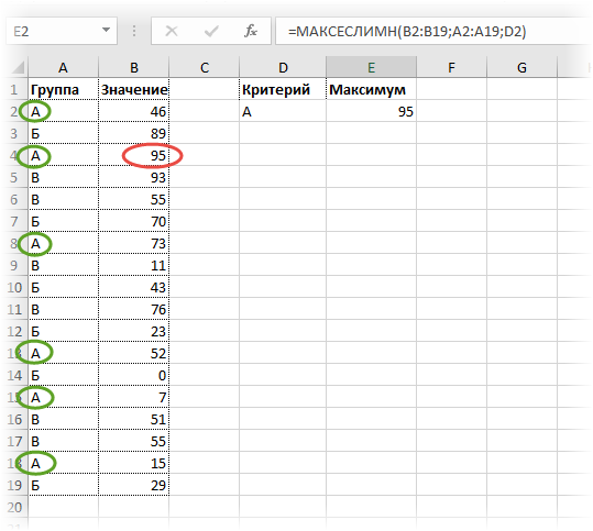
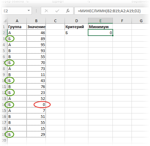
Все очень просто. Как и у СУММЕСЛИМН вначале указываем диапазон, где находится искомое максимальное значение (колонка В), затем диапазон с критериями (колонка А) и далее сам критерий (в ячейке D2). Можно указать сразу несколько условий. Таким же способом легко рассчитать минимальное значение по условию. Найдем, к примеру, минимум внутри группы Б.
Ниже показан
ролик, как рассчитать максимальное и минимальное значение по условию.
Поделиться в социальных сетях:
The MAXIFS Excel function is a statistics formula that returns the maximum value of only the cells that meet certain criteria. In this guide, we’re going to show you how to use the MAXIFS function and also go over some tips and error handling methods.
Supported Excel versions
- Excel 2016 and later
MAXIFS Function Syntax
MAXIFS(max_range, criteria_range1, criteria1, [criteria_range2, criteria2], …)
Arguments
|
max_range |
The range of values to be used to determine the maximum. |
|
criteria_range1 |
The range of cells that you want to apply the criteria1 against. |
|
criteria1 |
The criteria that is to be applied to criteria_range1 to define which cells are going to be evaluated as the maximum. |
|
[criteria_range2, criteria2] |
Optional. Additional ranges and their associated criteria pairs. You can enter up to 126 range/criteria pairs. |
Examples
Note that we’re using named ranges in our sample formulas to make them easier to read. This is not required.
Numeric condition
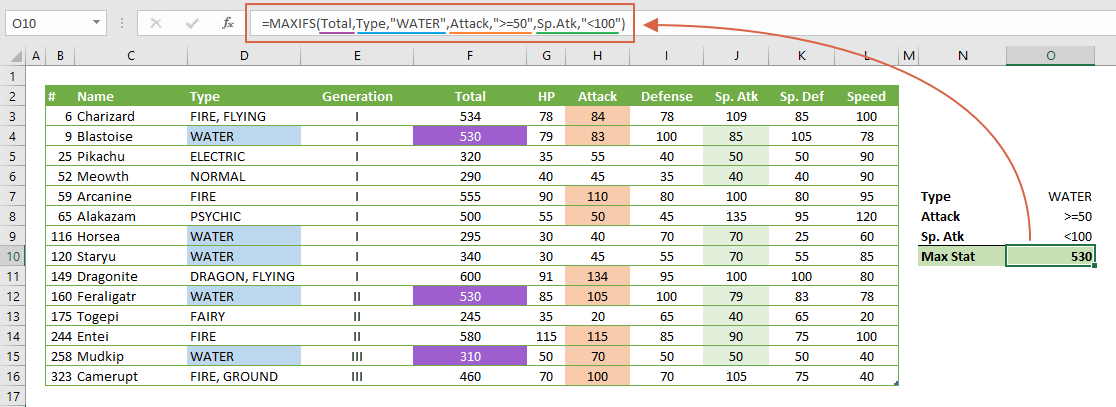
=MAXIFS(Total,Type,»WATER»,Attack,»>=50″,Sp.Atk,»<100″)
formula returns the maximum value from the named range Total, if the three conditions are satisfied. All conditions are combined with a logical and operation. As a result, only the values that meet all three criteria are evaluated for the maximum.
String criteria
=MAXIFS(HP,Type,»*FIRE*»,Generation,»<>I»)
formula determines the maximum value among the values where the Type contains the «FIRE» string, and Generation is not equal to «I». If we use «FIRE» only without asterisks, the MAXIFS function would ignore the «FIRE, GROUND» value.

Download Workbook
Tips
- Use the same number of rows and columns for max range and criteria range arguments.
- Bad Example: =MAXIFS(G2:G15,F2:H10,»>2014″,J2:J20,»IT»)
- Good Example: =MAXIFS(G2:G11,F2:F11,»>2014″,J2:J11,»IT»)
- Comparison operators:
|
Operator |
Description |
Criteria Sample |
Criteria Meaning |
|
= |
Equal to |
“=10000” |
Equal to 10000 |
|
<> |
Not equal to |
“<>10000” |
Not equal to 10000 |
|
> |
Greater than |
“>10000” |
Greater than 10000 |
|
< |
Less than |
“>10000” |
Less than 10000 |
|
>= |
Greater than or equal to |
“>=10000” |
Greater than or equal to 10000 |
|
<= |
Less than or equal to |
“<=10000” |
Less than or equal to 10000 |
|
? |
Takes the place of a single character |
“Admin?” |
6-character word starts by “Admin” |
|
* |
Can take the place of any number of characters. |
“Admin*” |
Any number of character word starts with “Admin” |
|
~ |
Use tilde in front of a question mark or an asterisk to actually find them |
“Admin~*” |
Equal to «Admin*» |
Note: Wildcards cannot be used for numeric values. Searching a wild card in a range of numeric values will return no matches.
Issues
#VALUE!
- The MAXIFS function returns incorrect results when you use it to match strings that are longer than 255 characters or to the string #VALUE!.
- If shape of max_range and criteria_range aren’t the same, MAXIFS returns the #VALUE! error.
TRUE and FALSE
TRUE and FALSE values in max_range are evaluated as numbers. While TRUE is evaluated as 1, FALSE is evaluated as 0. As a result this condition may cause unexpected results when evaluated as other values.
The MAXIFS function returns the largest numeric value that meets one or more supplied criteria. The MAXIFS function can apply criteria to dates, numbers, and text. MAXIFS supports logical operators (>,<,<>,=) and wildcards (*,?) for partial matching.
The MAXIFS function takes three required arguments: max_range, range1, and criteria1. With these three arguments, MAXIFS returns the maximum number in max_range where corresponding cells in range1 meet the condition set by criteria1. Additional conditions are applied using range/criteria pairs. The second condition is defined by range2 and criteria2, the third condition is range3 and criteria3, and so on. MAXIFS can handle up to 126 range/criteria pairs.
When using MAXIFS, keep the following in mind:
- Each new condition requires a separate range and criteria.
- To be included in the final result, all conditions must be TRUE.
- If no cells meet criteria, MAXIFS will return zero (0).
- MAXIFS will automatically ignore empty cells that meet criteria.
- MAXIFS requires a cell range for range arguments; you can’t use an array.
- MAXIFS will return a #VALUE! error if criteria_range is not the same size as max_range.
Criteria
The MAXIFS function supports logical operators (>,<,<>,=) and wildcards (*,?) for partial matching. Because MAXIFS is in a group of eight functions that split logical criteria into two parts, the syntax is a bit tricky. Each condition requires a separate range and criteria, and operators need to be enclosed in double quotes («»). The table below shows some common examples:
| Target | Criteria |
|---|---|
| Cells greater than 75 | «>75» |
| Cells equal to 100 | 100 or «100» |
| Cells less than or equal to 100 | «<=100» |
| Cells equal to «Red» | «red» |
| Cells not equal to «Red» | «<>red» |
| Cells that are blank «» | «» |
| Cells that are not blank | «<>» |
| Cells that begin with «X» | «x*» |
| Cells less than A1 | «<«&A1 |
| Cells less than today | «<«&TODAY() |
Notice the last two examples use concatenation with the ampersand (&) character. When a criteria argument includes a value from another cell, or the result of a formula, logical operators like «<» must be joined with concatenation. This is because Excel needs to evaluate cell references and formulas first to get a value before that value can be joined to an operator.
Basic Example
In the worksheet shown above, the formulas in G5 and G6 are:
=MAXIFS(D5:D16,C5:C16,"F") // returns 93
=MAXIFS(D5:D16,C5:C16,"M") // returns 83
In the first formula, MAXIFS returns the maximum value in D5:D16 where C5:C16 is equal to «F» (93). In the second formula, MAXIFS returns the maximum value in D5:D16 where C5:C16 is equal to «M» (83).
Two criteria
In the example below, the MAXIFS function is used with two criteria, one for Gender and one for Group. Note conditions are added in range/criteria pairs. The range E5:E16 is paired with the condition «B».

The formulas in H5:I6 are:
H5=MAXIFS(D5:D16,C5:C16,"F",E5:E16,"A") // returns 93
I5=MAXIFS(D5:D16,C5:C16,"F",E5:E16,"B") // returns 85
H6=MAXIFS(D5:D16,C5:C16,"M",E5:E16,"A") // returns 83
I6=MAXIFS(D5:D16,C5:C16,"M",E5:E16,"B") // returns 79
Other criteria
To return the maximum value in A1:A100 when cells in B1:B100 are greater than 50:
=MAXIFS(A1:A100,B1:B100,">50")
To get the maximum value in A1:A100 when cells in B1:B100 are less than or equal to 100, and cells in C1:C100 are greater than zero:
=MAXIFS(A1:A100,B1:B100,"<=100",C1:C100,">0")
Not equal to
To construct «not equal to» criteria, use the «<>» operator surrounded by double quotes («»). For example, to return the maximum value in A1:A100 when cells in B1:B100 are not equal to «red»:
=MAXIFS(A1:A100,B1:B100,"<>red")
Value from another cell
When using a value from another cell in a condition, the cell reference must be concatenated to the operator. For example, to return the maximum value in A1:A100 when cells in B1:B100 are greater than the value in C1:
=MAXIFS(A1:A100,B1:B100,">"&C1)
Notice the greater than operator (>) is enclosed in quotes («»), but the cell reference (C1) is not.
Wildcards
The wildcard characters question mark (?), asterisk(*), or tilde (~) can be used in criteria. A question mark (?) matches any one character, and an asterisk (*) matches zero or more characters. For example, to return the maximum value in A1:A100 when cells in B1:B100 begin with «a»:
=MAXIFS(A1:A100,B1:B100,"a*")
The tilde (~) is an escape character to allow you to find literal wildcards. For example, to match a literal question mark (?), asterisk(*), or tilde (~), add a tilde in front of the wildcard (i.e. ~?, ~*, ~~).
Notes
- Conditions are applied using range/criteria pairs.
- MAXIFS will return a #VALUE error if any criteria range is not the same size as max_range.
- If no criteria match, MAXIFS will return zero (0).
- MAXIFS ignores empty cells that meet criteria.