Функция from sheets excel - Word и Excel - помощь в работе с программами

If your Excel spreadsheet has a lot of data, consider using different sheets to organize them. To pull data from another sheet in Excel, follow this guide.

Excel doesn’t just let you work in one spreadsheet—you can create multiple sheets within the same file. This is useful if you want to keep your data separated. If you were running a business, you could decide to have sales information for each month on separate sheets, for example.

What if you want to use some of the data from one sheet in another, however? You could copy and paste it across, but this can be time-consuming. If you make changes to any of the original data, the data you copied across won’t be updated.

The good news is that it’s not too tricky to use the data from one sheet in another. Here’s how to pull data from another sheet in Excel.

How to Pull Data From Another Sheet in Excel Using Cell References

You can pull data from one Excel sheet to another by using the relevant cell references. This is a simple way to get data from one sheet into another.

To pull data from another sheet by using cell references in Excel:

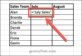
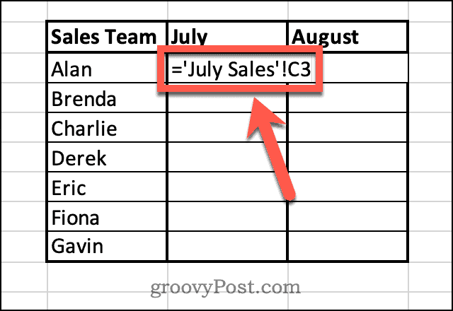
Click in the cell where you want the pulled data to appear.
Type = (equals sign) followed by the name of the sheet you want to pull data from. If the name of the sheet is more than one word, enclose the sheet name in single quotes.
Type ! followed by the cell reference of the cell you want to pull.
Press Enter.
The value from your other sheet will now appear in the cell.
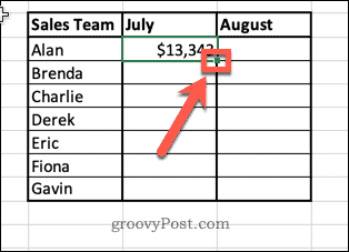
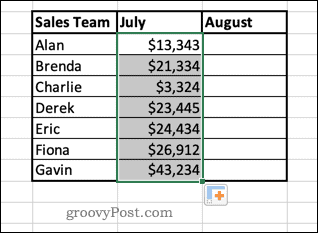
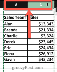
If you want to pull across more values, select the cell and hold the small square in the bottom-right corner of the cell.
Drag down to fill the remaining cells.

There is an alternative method that saves you from having to type in the cell references manually.

To pull data from another cell without typing the cell reference manually:

Click in the cell where you want the pulled data to appear.
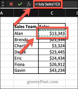
Type = (equals sign) and then open the sheet from which you want to pull data.
Click on the cell containing the data that you want to pull across. You’ll see the formula change to include the reference to this cell.
Press Enter and the data will be pulled into your cell.

The method above works well if you’re not planning to do much with your data and just want to put it into a new sheet. However, there are some issues if you start to manipulate the data.

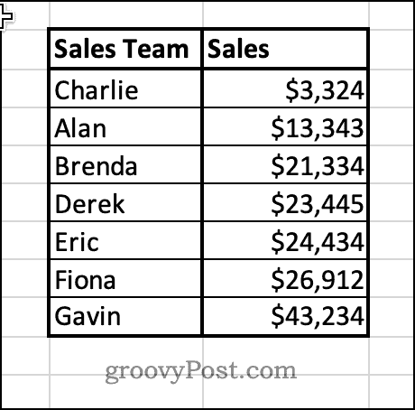
For example, if you sort the data in the July Sales sheet, the names of the sales team will also be rearranged.

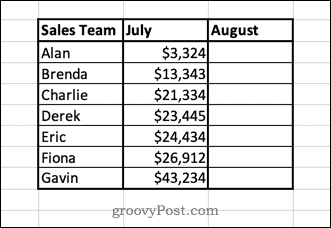
However, in the Sales Summary sheet, only the pulled data will change order. The other columns will remain the same, meaning that the sales are no longer aligned with the correct salesperson.

You can get around these issues by using the VLOOKUP function in Excel. Instead of pulling a value directly from a cell, this function pulls a value from a table that is in the same row as a unique identifier, such as the names in our example data. That means that even if the order of the original data changes, the data that is pulled will always remain the same.

To use VLOOKUP to pull data from another sheet in Excel:

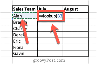
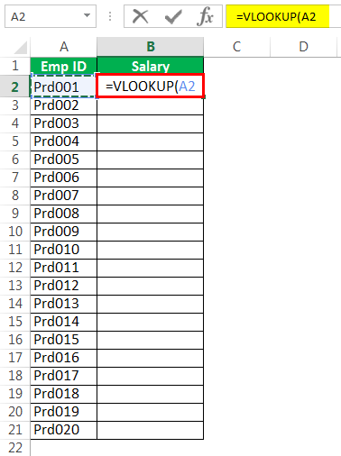
Click in the cell where you want the pulled data to appear.
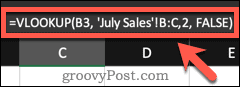
Type =VLOOKUP( then click on the cell to the left. This will be the reference that the VLOOKUP function will look for.
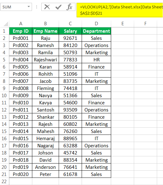
Type a comma, and then click on the sheet that you want to pull data from. Click and drag over the two columns that hold your data.
Type another comma, and then type the number of the column that contains the data you want to pull across. In this case, it’s the second column, so we would type 2.
Type another comma, then FALSE, then a final closed bracket to complete your formula. This ensures that the function looks for an exact match for your reference.
Press Enter. Your data will now appear in your cell.
If you want to pull across more values, select the cell and click and hold on the small square in the bottom right-hand corner of the cell.
Drag down to fill the remaining cells.
Now if you sort the original data, your pulled data will not change, since it is always looking for the data associated with each individual name.

Note that for this method to work, the unique identifiers (in this case, the names) must be in the first column of the range that you select.

Make Excel Work For You

There are hundreds of Excel functions that can take a lot of the grind out of your work and help you to do things quickly and easily. Knowing how to pull data from another sheet in Excel means you can say goodbye to endless copying and pasting.

Functions do have their limitations, however. As mentioned, this method will only work if your identifying data is in the first column. If your data is more complex, you’ll need to look into using other functions such as INDEX and MATCH.

VLOOKUP is a good place to start, however. If you’re having trouble with VLOOKUP, you should be able to troubleshoot VLOOKUP errors in Excel.

Источник

While working in Excel, we will often need to get values from another worksheet. This is possible by using the VLOOKUP function. In this tutorial, we will learn how to pull values from another worksheet in Excel, using VLOOKUP.

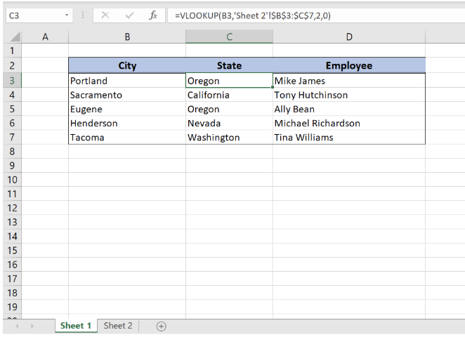
Figure 1. Final result

Syntax of the VLOOKUP formula

The generic formula for pulling values from another worksheet looks like:

=VLOOKUP(lookup_value, ’sheet_name’!range, col_index_num, range_lookup)

The parameters of the VLOOKUP function are:

lookup_value – a value that we want to find in another worksheet
’sheet_name’!range – a range in another worksheet in which we want to lookup
col_index_num – a column number in another worksheet from which we would like to pull a value
range_lookup – default value 0. This means that we want to find an exact match for a lookup value.

Setting up the Data

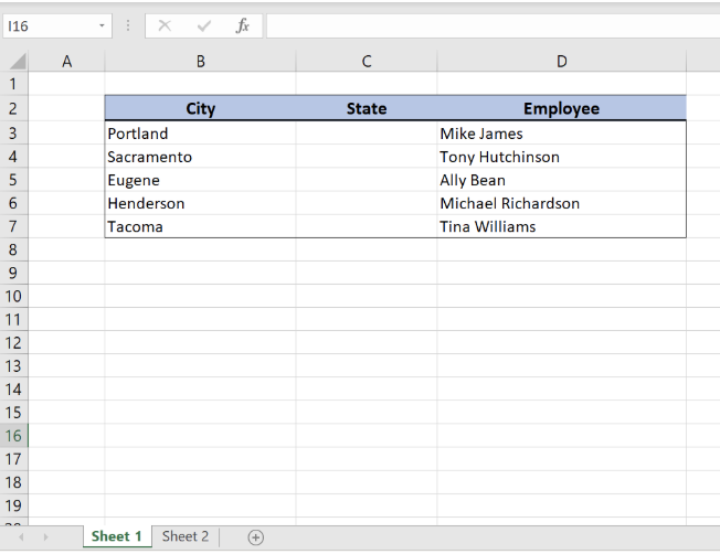Figure 2. “Sheet 1” in which we want to pull data

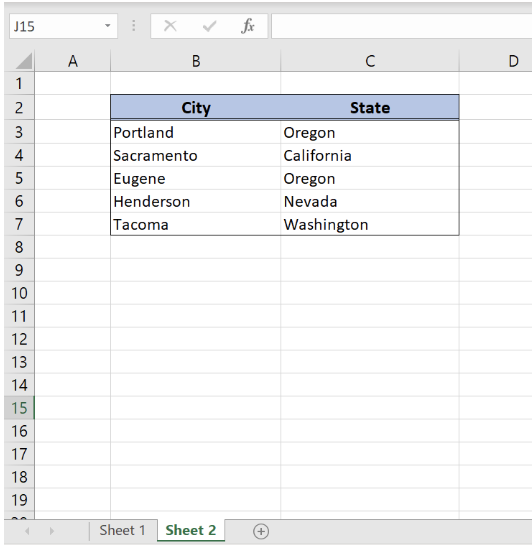Figure 3. Sheet 2 from which we want to pull data

We will now look at the example to explain in detail how this function works. Above all, let’s start with examining the structure of the data that we will use.

In “Sheet 1” we have a table in which we want to pull data, while in “Sheet2” we have the table from which we want to pull data. “Sheet 1” consists of “City” (column B), “State” (column C) and “Employee” (column D). “Sheet 2” consists of “City” (column B) and “State” (column C).

Get the State from Sheet 2 using VLOOKUP

Our goal is to obtain data from the “State” column in the second worksheet and populate it into the “State” column of the 1st worksheet. This will be done based on each corresponding city.

Figure 4. “Sheet 1” with pulled data in “State” column from “Sheet 2”

The formula looks like:

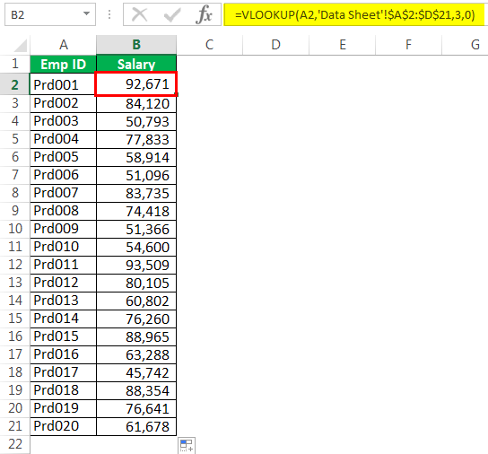
=VLOOKUP(B3,'Sheet 2'!$B$3:$C$7,2,0)

In our example, the lookup_value is the individual cell in “City” column. The parameter ’sheet_name’!range is ‘Sheet 2’!$B$3:$C$7 because we want to find value from the range B3:B7 in “Sheet 2”. Col_index_num has value 2, as we want to pull value from the second column of the range. Finally, range_lookup has value 0, because we want to find an exact match of “City” values.

Please note that we put absolute cell reference in table range ($ before B3:C7 range) as we must fix our lookup table.

To pull values from another worksheet, we need to follow these steps:

Select cell C3 and click on it
Insert the formula: =VLOOKUP(B3,'Sheet 2'!$B$3:$C$7,2,0)
Press enter
Drag the formula down to the other cells in the column by clicking and dragging the little “+” icon at the bottom-right of the cell.

As a result, we will get Oregon state in the cell B3. As you can see, the value of “City” in B3 on the “Sheet 1” is Portland, while in the “Sheet 2” state for Portland is Oregon. The function pulls this value and returns it to “Sheet 1” as a result.

Instant Connection to an Expert through our Excelchat Service:

Most of the time, the problem you will need to solve will be more complex than a simple application of a formula or function. If you want to save hours of research and frustration, try our live Excelchat service! Our Excel Experts are available 24/7 to answer any Excel question you may have. We guarantee a connection within 30 seconds and a customized solution within 20 minutes.

Are you still looking for help with the VLOOKUP function? View our comprehensive round-up of VLOOKUP function tutorials here.

Источник

Excel for Microsoft 365 for Mac Excel 2021 for Mac Excel 2019 for Mac Excel 2016 for Mac Excel for Mac 2011 More…Less

If you receive information in multiple sheets or workbooks that you want to summarize, the Consolidate command can help you pull data together onto one sheet. For example, if you have a sheet of expense figures from each of your regional offices, you might use a consolidation to roll up these figures into a corporate expense sheet. That sheet might contain sales totals and averages, current inventory levels, and highest selling products for the whole enterprise.

To decide which type of consolidation to use, look at the sheets you are combining. If the sheets have data in inconsistent positions, even if their row and column labels are not identical, consolidate by position. If the sheets use the same row and column labels for their categories, even if the data is not in consistent positions, consolidate by category.

Combine by position

For consolidation by position to work, the range of data on each source sheet must be in list format, without blank rows or blank columns in the list.

Open each source sheet and make sure that your data is in the same position on each sheet.
In your destination sheet, click the upper-left cell of the area where you want the consolidated data to appear.

Note: Make sure that you leave enough cells to the right and underneath for your consolidated data.
On the Data tab, in the Data Tools group, click Consolidate.
In the Function box, click the function that you want Excel to use to consolidate the data.
In each source sheet, select your data.

The file path is entered in All references.
When you have added the data from each source sheet and workbook, click OK.

Combine by category

For consolidation by category to work, the range of data on each source sheet must be in list format, without blank rows or blank columns in the list. Also the categories must be consistently labeled. For example, if one column is labeled Avg. and another is labeled Average, the Consolidate command will not sum the two columns together.

Open each source sheet.
In your destination sheet, click the upper-left cell of the area where you want the consolidated data to appear.

Note: Make sure that you leave enough cells to the right and underneath for your consolidated data.
On the Data tab, in the Data Tools group, click Consolidate.
In the Function box, click the function that you want Excel to use to consolidate the data.
To indicate where the labels are located in the source ranges, select the check boxes under Use labels in: either the Top row, the Left column, or both.
In each source sheet, select your data. Make sure to include either the top row or left column information that you previously selected.

The file path is entered in All references.
When you have added the data from each source sheet and workbook, click OK.

Note: Any labels that don’t match labels in the other source areas cause separate rows or columns in the consolidation.

Combine by position

For consolidation by position to work, the range of data on each source sheet must be in list format, without blank rows or blank columns in the list.

Open each source sheet and make sure that your data is in the same position on each sheet.
In your destination sheet, click the upper-left cell of the area where you want the consolidated data to appear.

Note: Make sure that you leave enough cells to the right and underneath for your consolidated data.
On the Data tab, under Tools, click Consolidate.
In the Function box, click the function that you want Excel to use to consolidate the data.
In each source sheet, select your data, and then click Add.

The file path is entered in All references.
When you have added the data from each source sheet and workbook, click OK.

Combine by category

Open each source sheet.
In your destination sheet, click the upper-left cell of the area where you want the consolidated data to appear.

Note: Make sure that you leave enough cells to the right and underneath for your consolidated data.
On the Data tab, under Tools, click Consolidate.
In the Function box, click the function that you want Excel to use to consolidate the data.
To indicate where the labels are located in the source ranges, select the check boxes under Use labels in: either the Top row, the Left column, or both.
In each source sheet, select your data. Make sure to include either the top row or left column information that you previously selected, and then click Add.

The file path is entered in All references.
When you have added the data from each source sheet and workbook, click OK.

Note: Any labels that don’t match labels in the other source areas cause separate rows or columns in the consolidation.

Need more help?

Want more options?

Explore subscription benefits, browse training courses, learn how to secure your device, and more.

Communities help you ask and answer questions, give feedback, and hear from experts with rich knowledge.

Источник

Vlookup is a function which can be used to reference columns from the same sheet or we can use it to refer it from another worksheet or from another workbook, the reference sheet is same as the reference cell but the table array and index number are chosen from a different workbook or different worksheet.

We all know the basics of the VLOOKUP functionThe VLOOKUP excel function searches for a particular value and returns a corresponding match based on a unique identifier. A unique identifier is uniquely associated with all the records of the database. For instance, employee ID, student roll number, customer contact number, seller email address, etc., are unique identifiers.
read more in excel. Probably for beginners level, you must have practiced the formula from the same sheet itself. Fetching the data from another worksheet or from another workbook is slightly different using the VLOOKUP function in excel.

Let us have a look at how to use VLOOKUP from another sheet and then how it can be used on another workbook.

How to Vlookup from Another Sheet / Workbook?
- #1 – VLOOKUP from Another Sheet but Same Workbook
- #2 – VLOOKUP from Different Workbook
- Things to Remember About Excel Vlookup from Another Sheet (Same or Different Workbook)
- Recommended Articles

#1 – VLOOKUP from Another Sheet but Same Workbook

Now copy the result table to another worksheet in the same workbook.

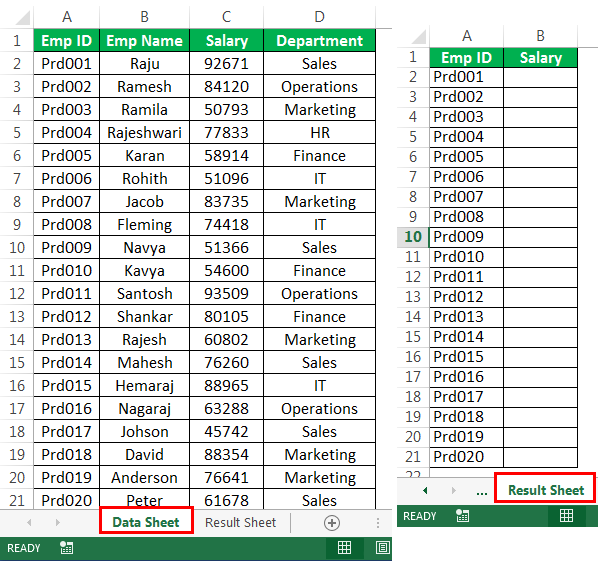
In the Result, Sheet opens the VLOOKUP formula and select the lookup value as cell A2.

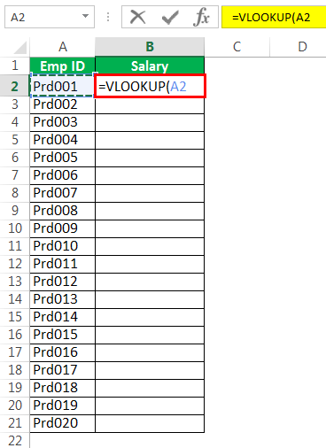
Now the table array is on a different sheet. Select the Data Sheet.

Now, look at the formula in the table array. It does not only contain table reference, but it contains the sheet name as well.

Note: Here, we need not need to type the sheet name manually. As soon as the cell in the other worksheet is selected, it automatically shows you the sheet name along with the cell reference of that sheet.

After selecting the range in the different worksheets, lock the range by typing the F4 key.

Now you need not go back to the actual worksheet where you are applying the formula rather here itself. You can finish the formula. Enter the column reference number and range lookup type.

We got the results from the other worksheet.

#2 – VLOOKUP from Different Workbook

We have seen how to fetch the data from a different worksheet in the same workbook. Now we will see how to fetch the data from a different workbook.

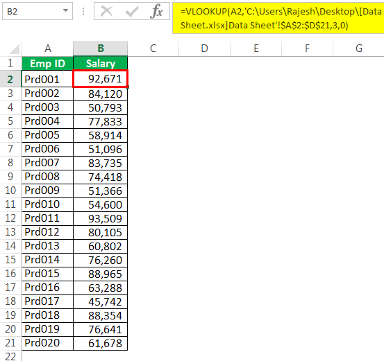
I have two workbooks; one is Data Workbook & Result Workbook.

From Data Workbook, I am fetching the data to Result Workbook.

Step 1: Open the VLOOKUP function in the Result workbook and select lookup value.

Step 2: Now go to the main data workbook and select the table array.

You can use Ctrl + Tab to switch between all the opened excel workbooks.

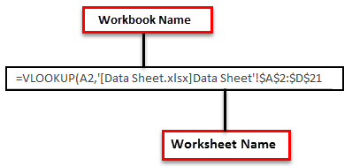
The table array not only contains table range rathbut it also, but it also contains Workbook Name, Worksheet Name, and data range in that workbook.

We need to lock the table array here. Excel itself locked the table array automatically.

Mention column index number and range lookup to get the result.

Now close the main workbook and see the formula.

It shows the path of the excel file we are referring to. It shows the complete file and subfile names.

We got the results.

Things to Remember About Excel Vlookup from Another Sheet (Same or Different Workbook)

We need to lock the table array range if you are fetching the data from the same worksheet or from different worksheets but from the same workbook.
We need to lock the table array range when the formula is applied to a different workbook. The formula automatically makes it an absolute referenceAbsolute reference in excel is a type of cell reference in which the cells being referred to do not change, as they did in relative reference. By pressing f4, we can create a formula for absolute referencing.read more.
Always remove VLOOKUP formulas if you are fetching the data from a different workbook. If you delete the workbook accidentally, you will lose all the data.

You can Download this Vlookup from Another Sheet or Workbook Excel template here – Vlookup from Another Sheet Excel Template.

SHEET and SHEETS functions in Excel: description of arguments and syntax

SHEETS function in Excel returns a numeric value that corresponds to the number of sheets referenced.

Notes:

Both functions are useful for use in documents containing a large number of sheets.
A sheet in Excel is a table of all the cells that are displayed on the screen and are outside of it (a total of 1,048,576 rows and 16,384 columns). When sending a sheet to print, it can be divided into several pages. Therefore, the terms “sheet” and “page” should not be confused.
The number of sheets in the book is limited only by the amount of PC RAM.

Function has only 1 argument in its syntax and is optional for: =SHEET(value).

value is an optional function argument that contains text data with the name of the sheet or a link for which you want to set the sheet number. If this parameter is not specified, the function will return the number of the sheet in one of the cells of which it was written.

Notes:

When the sheet works, all sheets that are visible, hidden and very hidden are taken into account. Exceptions are dialogs, macros, and diagrams.
If the function argument is a text value that does not match the name of any of the sheets contained in the book, the error #NA will be returned.
If an invalid value was passed as an argument to the function, the result of its calculation will be the error #REF!.
Within the object model (the hierarchy of objects in VBA, in which Application is the main object and Workbook, WorkSheet, etc., are child objects), the SHEET function is not available because it contains a similar function.

The function has the following syntax: =SHEETS(reference).

reference — an object of reference type for which you want to determine the number of sheets. This argument is optional. If this parameter is not specified, the function will return the number of sheets contained in the book where it was written.

Notes:

This function counts the number of all hidden, very hidden and visible sheets, with the exception of charts, macros and dialogs.
If an invalid reference was passed as a parameter, the result of the calculation is the error code #REF!.
This function is not available in the object model due to the presence of a similar function there.

How to get sheet name by formula in Excel

Example 1. In carrying out the calculated work the student used the Excel program, in which he created a book of several sheets. For his own convenience, the student decided to display in the cells A2 and B2 of each sheet data on the name of the sheet and its serial number, respectively. For this, he used the following formulas:

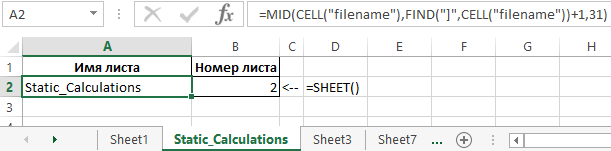
Description of arguments for the MID function:

=CELL(«filename») is a function that returns text in which the MID function searches for a specified number of characters. In this case, the value “C:UserssoulpDesktop[Workbook.xlsx] Static_Calculations” will return, where after the “]” symbol is the required text — the name.
=FIND(«]»,CELL(«filename»))+1 is a function that returns the position number of the character «]», one is added so that the MID function does not take into account the character].
31 — the maximum number of characters in the name.

=SHEET() — this function without parameter returns the number of the current sheet. As a result of its calculation, we get the number of sheets in the current book.

Examples of using the SHEET function and SHEETS

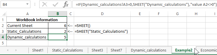
Example 2. The Excel workbook contains several sheets. It is necessary:

Return the current sheet number.
Return the sheet number with the name «Static_calculations».
Return the number of the sheet «Dynamic_calculations», if its cell A3 contains the value 0.

Enter the data in the table:

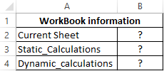
Next, we write the formulas for all 4 conditions:

For condition # 1, use the following formula: =SHEET()
For condition # 2, enter the formula: =SHEET(«Static_calculations»)
For condition number 3 we write the formula:

The IF function checks whether the value stored in the A3 cell of the Dynamic_ calculations is equal to zero or null.

As a result, we get:

Processing information about the sheets of the book on the formula Excel

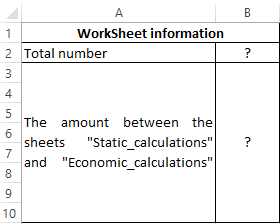
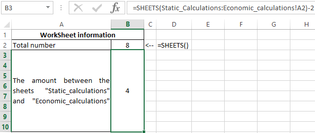
Example 3. To determine the contains several sheets. It is necessary to determine the total number of sheets, as well as the number contained between the “Static_calculations” and “Economic_calculations”.

The source table is:

The total number of sheets is calculated by the formula:

To determine the number contained between these two sheets, we write the formula:

Static_calculations: Economic_calculations!A2 — A reference to cell A2 of the range of sheets between «Static_calculations» and «Economic_calculations» including these sheets.
To get the desired value, 2 was subtracted.

As a result, we get the following:

Download examples SHEET and SHEETS functions in Excel formulas

The formula displays detailed information on the data on the sheets in a certain range of their location in the Excel workbook.

Источник

How to Pull Data From Another Sheet in Excel Using Cell References

Make Excel Work For You

Syntax of the VLOOKUP formula

Setting up the Data

Get the State from Sheet 2 using VLOOKUP

Instant Connection to an Expert through our Excelchat Service:

Combine by position

Combine by category

Combine by position

Combine by category

Need more help?

Want more options?

Table of contents

#1 – VLOOKUP from Another Sheet but Same Workbook

#2 – VLOOKUP from Different Workbook

Things to Remember About Excel Vlookup from Another Sheet (Same or Different Workbook)

Recommended Articles

SHEET and SHEETS functions in Excel: description of arguments and syntax

How to get sheet name by formula in Excel

Examples of using the SHEET function and SHEETS

Processing information about the sheets of the book on the formula Excel