
Microsoft Excel → Page 2
Microsoft Excel solved MCQ sets : MS Excel Questions Answers (MCQ -Multiple Choice, Objective Type) Online test : Microsoft Excel is a spreadsheet software and is part of the widely used MS Office Package. Here you will find a great collection of Multiple Choice (MCQ)Questions in the category of Microsoft Excel with answer. Most of the questions are applicable to all versions of M…READ MORE
TEST INSTRUCTION: CLICK OPTION (A, B, C, D) TO SEE ANSWER.
| Q. |
1. What type of chart will you use to compare performance of two employees in the year 2016 ?Show Answer |
| Q. |
2. Which one is not a Function in MS Excel ?Show Answer |
| Q. |
3. Functions in MS Excel must begin with ___Show Answer |
| Q. |
4. Which functionin Excel checks whether a condition is true or not ?Show Answer |
| Q. |
5. In Excel, Columns are labelled as ___Show Answer |
Advertisement
Search Here
Содержание
- Using functions and nested functions in Excel formulas
- Use nested functions in a formula
- Examples
- Using functions and nested functions in Excel formulas
- Overview of formulas in Excel
- Create a formula that refers to values in other cells
- See a formula
- Enter a formula that contains a built-in function
- Download our Formulas tutorial workbook
- Formulas in-depth
- Need more help?
Using functions and nested functions in Excel formulas
Functions are predefined formulas that perform calculations by using specific values, called arguments, in a particular order, or structure. Functions can be used to perform simple or complex calculations. You can find all of Excel’s functions on the Formulas tab on the Ribbon:

Excel function syntax
The following example of the ROUND function rounding off a number in cell A10 illustrates a function’s syntax.
1. Structure. The structure of a function begins with an equal sign (=), followed by the function name, an opening parenthesis, the arguments for the function separated by commas, and a closing parenthesis.
2. Function name. For a list of available functions, click a cell and press SHIFT+F3, which will launch the Insert Function dialog.

3. Arguments. Arguments can be numbers, text, logical values such as TRUE or FALSE, arrays, error values such as #N/A, or cell references. The argument you designate must produce a valid value for that argument. Arguments can also be constants, formulas, or other functions.
4. Argument tooltip. A tooltip with the syntax and arguments appears as you type the function. For example, type =ROUND( and the tooltip appears. Tooltips appear only for built-in functions.
Note: You don’t need to type functions in all caps, like =ROUND, as Excel will automatically capitalize the function name for you once you press enter. If you misspell a function name, like =SUME(A1:A10) instead of =SUM(A1:A10), then Excel will return a #NAME? error.
Entering Excel functions
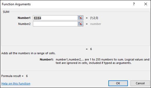
When you create a formula that contains a function, you can use the Insert Function dialog box to help you enter worksheet functions. Once you select a function from the Insert Function dialog Excel will launch a function wizard, which displays the name of the function, each of its arguments, a description of the function and each argument, the current result of the function, and the current result of the entire formula.
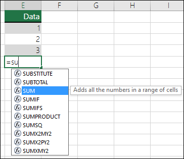
To make it easier to create and edit formulas and minimize typing and syntax errors, use Formula AutoComplete. After you type an = (equal sign) and beginning letters of a function, Excel displays a dynamic drop-down list of valid functions, arguments, and names that match those letters. You can then select one from the drop-down list and Excel will enter it for you.
Nesting Excel functions
In certain cases, you may need to use a function as one of the arguments of another function. For example, the following formula uses a nested AVERAGE function and compares the result with the value 50.
1. The AVERAGE and SUM functions are nested within the IF function.
Valid returns When a nested function is used as an argument, the nested function must return the same type of value that the argument uses. For example, if the argument returns a TRUE or FALSE value, the nested function must return a TRUE or FALSE value. If the function doesn’t, Excel displays a #VALUE! error value.
Nesting level limits A formula can contain up to seven levels of nested functions. When one function (we’ll call this Function B) is used as an argument in another function (we’ll call this Function A), Function B acts as a second-level function. For example, the AVERAGE function and the SUM function are both second-level functions if they are used as arguments of the IF function. A function nested within the nested AVERAGE function is then a third-level function, and so on.
Источник
Use nested functions in a formula
Using a function as one of the arguments in a formula that uses a function is called nesting, and we’ll refer to that function as a nested function. For example, by nesting the AVERAGE and SUM function in the arguments of the IF function, the following formula sums a set of numbers (G2:G5) only if the average of another set of numbers (F2:F5) is greater than 50. Otherwise, it returns 0.
The AVERAGE and SUM functions are nested within the IF function.
You can nest up to 64 levels of functions in a formula.
Click the cell in which you want to enter the formula.
To start the formula with the function, click Insert Function  on the formula bar
  .
.
Excel inserts the equal sign ( =) for you.
In the Or select a category box, select All.
If you are familiar with the function categories, you can also select a category.
If you’re not sure which function to use, you can type a question that describes what you want to do in the Search for a function box (for example, «add numbers» returns the SUM function).
To enter another function as an argument, enter the function in the argument box that you want.
The parts of the formula displayed in the Function Arguments dialog box reflect the function that you selected in the previous step.
If you clicked IF, the Function arguments dialog box displays the arguments for the IF function. To nest another function, you can enter it into the argument box. For example, you could enter SUM(G2:G5) in the Value_if_true box of the IF function.
Enter any additional arguments that are needed to complete your formula.
Instead of typing cell references, you can also select the cells that you want to reference. Click  to minimize the dialog box, select the cells you want to reference, and then click
  to expand the dialog box again.
Tip: For more information about the function and its arguments, click Help on this function.
After you complete the arguments for the formula, click OK.
Click the cell in which you want to enter the formula.
To start the formula with the function, click Insert Function on the formula bar .
In the Insert Function dialog box, in the Pick a category box, select All.
If you are familiar with the function categories, you can also select a category.
To enter another function as an argument, enter the function in the argument box in the Formula Builder or directly into the cell.
Enter any additional arguments that are needed to complete your formula.
After you complete the arguments for the formula, press ENTER.
Examples
The following shows an example of using nested IF functions to assign a letter grade to a numeric test score.
Copy the example data in the following table, and paste it in cell A1 of a new Excel worksheet. For formulas to show results, select them, press F2, and then press Enter. If you need to, you can adjust the column widths to see all the data.
Источник
Using functions and nested functions in Excel formulas
Functions are predefined formulas that perform calculations by using specific values, called arguments, in a particular order, or structure. Functions can be used to perform simple or complex calculations. You can find all of Excel’s functions on the Formulas tab on the Ribbon:
Excel function syntax
The following example of the ROUND function rounding off a number in cell A10 illustrates a function’s syntax.
1. Structure. The structure of a function begins with an equal sign (=), followed by the function name, an opening parenthesis, the arguments for the function separated by commas, and a closing parenthesis.
2. Function name. For a list of available functions, click a cell and press SHIFT+F3, which will launch the Insert Function dialog.
3. Arguments. Arguments can be numbers, text, logical values such as TRUE or FALSE, arrays, error values such as #N/A, or cell references. The argument you designate must produce a valid value for that argument. Arguments can also be constants, formulas, or other functions.
4. Argument tooltip. A tooltip with the syntax and arguments appears as you type the function. For example, type =ROUND( and the tooltip appears. Tooltips appear only for built-in functions.
Note: You don’t need to type functions in all caps, like =ROUND, as Excel will automatically capitalize the function name for you once you press enter. If you misspell a function name, like =SUME(A1:A10) instead of =SUM(A1:A10), then Excel will return a #NAME? error.
Entering Excel functions
When you create a formula that contains a function, you can use the Insert Function dialog box to help you enter worksheet functions. Once you select a function from the Insert Function dialog Excel will launch a function wizard, which displays the name of the function, each of its arguments, a description of the function and each argument, the current result of the function, and the current result of the entire formula.
To make it easier to create and edit formulas and minimize typing and syntax errors, use Formula AutoComplete. After you type an = (equal sign) and beginning letters of a function, Excel displays a dynamic drop-down list of valid functions, arguments, and names that match those letters. You can then select one from the drop-down list and Excel will enter it for you.
Nesting Excel functions
In certain cases, you may need to use a function as one of the arguments of another function. For example, the following formula uses a nested AVERAGE function and compares the result with the value 50.
1. The AVERAGE and SUM functions are nested within the IF function.
Valid returns When a nested function is used as an argument, the nested function must return the same type of value that the argument uses. For example, if the argument returns a TRUE or FALSE value, the nested function must return a TRUE or FALSE value. If the function doesn’t, Excel displays a #VALUE! error value.
Nesting level limits A formula can contain up to seven levels of nested functions. When one function (we’ll call this Function B) is used as an argument in another function (we’ll call this Function A), Function B acts as a second-level function. For example, the AVERAGE function and the SUM function are both second-level functions if they are used as arguments of the IF function. A function nested within the nested AVERAGE function is then a third-level function, and so on.
Источник
Overview of formulas in Excel
Get started on how to create formulas and use built-in functions to perform calculations and solve problems.

Important: The calculated results of formulas and some Excel worksheet functions may differ slightly between a Windows PC using x86 or x86-64 architecture and a Windows RT PC using ARM architecture. Learn more about the differences.
Important: In this article we discuss XLOOKUP and VLOOKUP, which are similar. Try using the new XLOOKUP function, an improved version of VLOOKUP that works in any direction and returns exact matches by default, making it easier and more convenient to use than its predecessor.
Create a formula that refers to values in other cells
Type the equal sign =.
Note: Formulas in Excel always begin with the equal sign.
Select a cell or type its address in the selected cell.

Enter an operator. For example, – for subtraction.
Select the next cell, or type its address in the selected cell.

Press Enter. The result of the calculation appears in the cell with the formula.
See a formula
When a formula is entered into a cell, it also appears in the Formula bar.

To see a formula, select a cell, and it will appear in the formula bar.

Enter a formula that contains a built-in function
Select an empty cell.
Type an equal sign = and then type a function. For example, =SUM for getting the total sales.
Type an opening parenthesis (.
Select the range of cells, and then type a closing parenthesis).

Press Enter to get the result.
Download our Formulas tutorial workbook
We’ve put together a Get started with Formulas workbook that you can download. If you’re new to Excel, or even if you have some experience with it, you can walk through Excel’s most common formulas in this tour. With real-world examples and helpful visuals, you’ll be able to Sum, Count, Average, and Vlookup like a pro.
Formulas in-depth
You can browse through the individual sections below to learn more about specific formula elements.
A formula can also contain any or all of the following: functions, references, operators, and constants.
Parts of a formula

1. Functions: The PI() function returns the value of pi: 3.142.
2. References: A2 returns the value in cell A2.
3. Constants: Numbers or text values entered directly into a formula, such as 2.
4. Operators: The ^ (caret) operator raises a number to a power, and the * (asterisk) operator multiplies numbers.
A constant is a value that is not calculated; it always stays the same. For example, the date 10/9/2008, the number 210, and the text «Quarterly Earnings» are all constants. An expression or a value resulting from an expression is not a constant. If you use constants in a formula instead of references to cells (for example, =30+70+110), the result changes only if you modify the formula. In general, it’s best to place constants in individual cells where they can be easily changed if needed, then reference those cells in formulas.
A reference identifies a cell or a range of cells on a worksheet, and tells Excel where to look for the values or data you want to use in a formula. You can use references to use data contained in different parts of a worksheet in one formula or use the value from one cell in several formulas. You can also refer to cells on other sheets in the same workbook, and to other workbooks. References to cells in other workbooks are called links or external references.
The A1 reference style
By default, Excel uses the A1 reference style, which refers to columns with letters (A through XFD, for a total of 16,384 columns) and refers to rows with numbers (1 through 1,048,576). These letters and numbers are called row and column headings. To refer to a cell, enter the column letter followed by the row number. For example, B2 refers to the cell at the intersection of column B and row 2.
The cell in column A and row 10
The range of cells in column A and rows 10 through 20
The range of cells in row 15 and columns B through E
All cells in row 5
All cells in rows 5 through 10
All cells in column H
All cells in columns H through J
The range of cells in columns A through E and rows 10 through 20
Making a reference to a cell or a range of cells on another worksheet in the same workbook
In the following example, the AVERAGE function calculates the average value for the range B1:B10 on the worksheet named Marketing in the same workbook.

1. Refers to the worksheet named Marketing
2. Refers to the range of cells from B1 to B10
3. The exclamation point (!) Separates the worksheet reference from the cell range reference
Note: If the referenced worksheet has spaces or numbers in it, then you need to add apostrophes (‘) before and after the worksheet name, like =’123′!A1 or =’January Revenue’!A1.
The difference between absolute, relative and mixed references
Relative references A relative cell reference in a formula, such as A1, is based on the relative position of the cell that contains the formula and the cell the reference refers to. If the position of the cell that contains the formula changes, the reference is changed. If you copy or fill the formula across rows or down columns, the reference automatically adjusts. By default, new formulas use relative references. For example, if you copy or fill a relative reference in cell B2 to cell B3, it automatically adjusts from =A1 to =A2.
Copied formula with relative reference

Absolute references An absolute cell reference in a formula, such as $A$1, always refer to a cell in a specific location. If the position of the cell that contains the formula changes, the absolute reference remains the same. If you copy or fill the formula across rows or down columns, the absolute reference does not adjust. By default, new formulas use relative references, so you may need to switch them to absolute references. For example, if you copy or fill an absolute reference in cell B2 to cell B3, it stays the same in both cells: =$A$1.
Copied formula with absolute reference

Mixed references A mixed reference has either an absolute column and relative row, or absolute row and relative column. An absolute column reference takes the form $A1, $B1, and so on. An absolute row reference takes the form A$1, B$1, and so on. If the position of the cell that contains the formula changes, the relative reference is changed, and the absolute reference does not change. If you copy or fill the formula across rows or down columns, the relative reference automatically adjusts, and the absolute reference does not adjust. For example, if you copy or fill a mixed reference from cell A2 to B3, it adjusts from =A$1 to =B$1.
Copied formula with mixed reference

The 3-D reference style
Conveniently referencing multiple worksheets If you want to analyze data in the same cell or range of cells on multiple worksheets within a workbook, use a 3-D reference. A 3-D reference includes the cell or range reference, preceded by a range of worksheet names. Excel uses any worksheets stored between the starting and ending names of the reference. For example, =SUM(Sheet2:Sheet13!B5) adds all the values contained in cell B5 on all the worksheets between and including Sheet 2 and Sheet 13.
You can use 3-D references to refer to cells on other sheets, to define names, and to create formulas by using the following functions: SUM, AVERAGE, AVERAGEA, COUNT, COUNTA, MAX, MAXA, MIN, MINA, PRODUCT, STDEV.P, STDEV.S, STDEVA, STDEVPA, VAR.P, VAR.S, VARA, and VARPA.
3-D references cannot be used in array formulas.
3-D references cannot be used with the intersection operator (a single space) or in formulas that use implicit intersection.
What occurs when you move, copy, insert, or delete worksheets The following examples explain what happens when you move, copy, insert, or delete worksheets that are included in a 3-D reference. The examples use the formula =SUM(Sheet2:Sheet6!A2:A5) to add cells A2 through A5 on worksheets 2 through 6.
Insert or copy If you insert or copy sheets between Sheet2 and Sheet6 (the endpoints in this example), Excel includes all values in cells A2 through A5 from the added sheets in the calculations.
Delete If you delete sheets between Sheet2 and Sheet6, Excel removes their values from the calculation.
Move If you move sheets from between Sheet2 and Sheet6 to a location outside the referenced sheet range, Excel removes their values from the calculation.
Move an endpoint If you move Sheet2 or Sheet6 to another location in the same workbook, Excel adjusts the calculation to accommodate the new range of sheets between them.
Delete an endpoint If you delete Sheet2 or Sheet6, Excel adjusts the calculation to accommodate the range of sheets between them.
The R1C1 reference style
You can also use a reference style where both the rows and the columns on the worksheet are numbered. The R1C1 reference style is useful for computing row and column positions in macros. In the R1C1 style, Excel indicates the location of a cell with an «R» followed by a row number and a «C» followed by a column number.
A relative reference to the cell two rows up and in the same column
A relative reference to the cell two rows down and two columns to the right
An absolute reference to the cell in the second row and in the second column
A relative reference to the entire row above the active cell
An absolute reference to the current row
When you record a macro, Excel records some commands by using the R1C1 reference style. For example, if you record a command, such as clicking the AutoSum button to insert a formula that adds a range of cells, Excel records the formula by using R1C1 style, not A1 style, references.
You can turn the R1C1 reference style on or off by setting or clearing the R1C1 reference style check box under the Working with formulas section in the Formulas category of the Options dialog box. To display this dialog box, click the File tab.
Need more help?
You can always ask an expert in the Excel Tech Community or get support in the Answers community.
Источник
Question :- Functions is MS-Excel must begin with
Solution :- Excel formulas are helpful in various mathematical, statistical and logical operations. You can either type in a formula, but you need to make sure it is correct, or use Excel’s preset functions called functions.
To make Excel recognize that you are entering a formula, it is necessary to start your formula with an equal sign. Depending on the task you are trying to accomplish, the next step is determined by what you did. To multiply numbers, simply type the numbers and symbol (* to multiply strong>
Excel can also perform more complicated calculations. This includes calculations for the cell, regardless of its content (for instance, if it changes from a 5 or a 8), as well as complex formulas (such averages, sums and other math beyond basic math). You must start with an equal sign, just like in a basic formula. The function name would be followed by the range of cells within parentheses. A colon would then separate them. Example: =SUM(B2 : B5). Excel comes with many pre-defined functions so that you don’t need to remember what you have to do. Just remember the name.
What is Fatskills?
Our mission is to help you improve your basic knowledge of any subject and exam using online quizzes, practice tests & study guides.
18.5k Practice Tests / Practice Exams and Online Quizzes.
1.65 Million+ Multiple Choice Test Questions / Practice Questions
700+ Subjects Covering All Test Prep, Competitive Exams, Certification Exams, Entrance Exams, & School / College Exams.
Browse Fatskills
Test Prep For Top Exams: SAT | ACT | IELTS | GMAT | GRE | GED | ASVAB
Test Prep For Competitive Exams: English For Competitive Exams | Quantitative Aptitude and Numerical Ability For Competitive Exams | Reasoning For Competitive Exams | Math For Competitive Exams | General Studies For Competitive Exams | Commerce For Competitive Exams | Computer Fundamentals For Competitive Exams | General Knowledge
Test Prep For Popular Tests: Citizenship Test | Driving Test | Popular Tests on Fatskills
Subjects: Aptitude | Basic Life Skills | High School | Elementary School | Entrance and Placement Exams | Jobs and Occupations | Information Technology | Certifications | Business Skills | Trades and Vocational | Languages | English | Healthcare | Math | Science and Technology | Education Standards and Boards | Humanities | Law
Explore: Popular Tests on Fatskills | Best of Fatskills | Basic Literacy Skills | 700+ Classes on Fatskills | Favorite Quizzes & Guides | Browse Fatskills by topics | All Subjects on Fatskills | Fatskills Career Aptitude Tests | Fatskills Community
Fatskills
About Fatskills | Benefits of Quizzes | Help | Privacy Policy | Terms of Use | Twitter | Facebook | Telegram | Reddit
Just like a basic formula, you need to start with the equal sign. After that, you would put the function name, then the range of cells inside parentheses, separated with a colon. For example: =SUM(B2:B5).
Related Posts:
- Is there a Business Day function in Excel?
— The NETWORKDAYS Function calculates the number of… (Read More) - How do I list business days in Excel?
— In Excel, you can list weekdays with… (Read More) - How do you get to the next business day in Excel?
— To get the next working day, or… (Read More) - How do I use workday in Excel?
— Excel WORKDAY FunctionSummary. … Get a date… (Read More) - How do you add 5 business days in Excel?
— Add business days excluding weekends with formula… (Read More) - How do I subtract business days in Excel?
— How to use WORKDAY to add /… (Read More) - Which type of charts can excel produce?
— Excel Charts — TypesColumn Chart.Line Chart.Pie Chart.Doughnut… (Read More) - What is the file extension for Excel?
— What is an Excel file extension?Excel File… (Read More) - How many seats are there in Excel?
— How many sheets, rows, and columns can… (Read More) - How do you display the current date in Excel?
— There are two ways to enter the… (Read More)