
Summary
This step-by-step article describes how to find data in a table (or range of cells) by using various built-in functions in Microsoft Excel. You can use different formulas to get the same result.
Create the Sample Worksheet
This article uses a sample worksheet to illustrate Excel built-in functions. Consider the example of referencing a name from column A and returning the age of that person from column C. To create this worksheet, enter the following data into a blank Excel worksheet.
You will type the value that you want to find into cell E2. You can type the formula in any blank cell in the same worksheet.
|
A |
B |
C |
D |
E |
||
|
1 |
Name |
Dept |
Age |
Find Value |
||
|
2 |
Henry |
501 |
28 |
Mary |
||
|
3 |
Stan |
201 |
19 |
|||
|
4 |
Mary |
101 |
22 |
|||
|
5 |
Larry |
301 |
29 |
Term Definitions
This article uses the following terms to describe the Excel built-in functions:
|
Term |
Definition |
Example |
|
Table Array |
The whole lookup table |
A2:C5 |
|
Lookup_Value |
The value to be found in the first column of Table_Array. |
E2 |
|
Lookup_Array |
The range of cells that contains possible lookup values. |
A2:A5 |
|
Col_Index_Num |
The column number in Table_Array the matching value should be returned for. |
3 (third column in Table_Array) |
|
Result_Array |
A range that contains only one row or column. It must be the same size as Lookup_Array or Lookup_Vector. |
C2:C5 |
|
Range_Lookup |
A logical value (TRUE or FALSE). If TRUE or omitted, an approximate match is returned. If FALSE, it will look for an exact match. |
FALSE |
|
Top_cell |
This is the reference from which you want to base the offset. Top_Cell must refer to a cell or range of adjacent cells. Otherwise, OFFSET returns the #VALUE! error value. |
|
|
Offset_Col |
This is the number of columns, to the left or right, that you want the upper-left cell of the result to refer to. For example, «5» as the Offset_Col argument specifies that the upper-left cell in the reference is five columns to the right of reference. Offset_Col can be positive (which means to the right of the starting reference) or negative (which means to the left of the starting reference). |
Functions
LOOKUP()
The LOOKUP function finds a value in a single row or column and matches it with a value in the same position in a different row or column.
The following is an example of LOOKUP formula syntax:
=LOOKUP(Lookup_Value,Lookup_Vector,Result_Vector)
The following formula finds Mary’s age in the sample worksheet:
=LOOKUP(E2,A2:A5,C2:C5)
The formula uses the value «Mary» in cell E2 and finds «Mary» in the lookup vector (column A). The formula then matches the value in the same row in the result vector (column C). Because «Mary» is in row 4, LOOKUP returns the value from row 4 in column C (22).
NOTE: The LOOKUP function requires that the table be sorted.
For more information about the LOOKUP function, click the following article number to view the article in the Microsoft Knowledge Base:
How to use the LOOKUP function in Excel
VLOOKUP()
The VLOOKUP or Vertical Lookup function is used when data is listed in columns. This function searches for a value in the left-most column and matches it with data in a specified column in the same row. You can use VLOOKUP to find data in a sorted or unsorted table. The following example uses a table with unsorted data.
The following is an example of VLOOKUP formula syntax:
=VLOOKUP(Lookup_Value,Table_Array,Col_Index_Num,Range_Lookup)
The following formula finds Mary’s age in the sample worksheet:
=VLOOKUP(E2,A2:C5,3,FALSE)
The formula uses the value «Mary» in cell E2 and finds «Mary» in the left-most column (column A). The formula then matches the value in the same row in Column_Index. This example uses «3» as the Column_Index (column C). Because «Mary» is in row 4, VLOOKUP returns the value from row 4 in column C (22).
For more information about the VLOOKUP function, click the following article number to view the article in the Microsoft Knowledge Base:
How to Use VLOOKUP or HLOOKUP to find an exact match
INDEX() and MATCH()
You can use the INDEX and MATCH functions together to get the same results as using LOOKUP or VLOOKUP.
The following is an example of the syntax that combines INDEX and MATCH to produce the same results as LOOKUP and VLOOKUP in the previous examples:
=INDEX(Table_Array,MATCH(Lookup_Value,Lookup_Array,0),Col_Index_Num)
The following formula finds Mary’s age in the sample worksheet:
=INDEX(A2:C5,MATCH(E2,A2:A5,0),3)
The formula uses the value «Mary» in cell E2 and finds «Mary» in column A. It then matches the value in the same row in column C. Because «Mary» is in row 4, the formula returns the value from row 4 in column C (22).
NOTE: If none of the cells in Lookup_Array match Lookup_Value («Mary»), this formula will return #N/A.
For more information about the INDEX function, click the following article number to view the article in the Microsoft Knowledge Base:
How to use the INDEX function to find data in a table
OFFSET() and MATCH()
You can use the OFFSET and MATCH functions together to produce the same results as the functions in the previous example.
The following is an example of syntax that combines OFFSET and MATCH to produce the same results as LOOKUP and VLOOKUP:
=OFFSET(top_cell,MATCH(Lookup_Value,Lookup_Array,0),Offset_Col)
This formula finds Mary’s age in the sample worksheet:
=OFFSET(A1,MATCH(E2,A2:A5,0),2)
The formula uses the value «Mary» in cell E2 and finds «Mary» in column A. The formula then matches the value in the same row but two columns to the right (column C). Because «Mary» is in column A, the formula returns the value in row 4 in column C (22).
For more information about the OFFSET function, click the following article number to view the article in the Microsoft Knowledge Base:
How to use the OFFSET function
Need more help?
Want more options?
Explore subscription benefits, browse training courses, learn how to secure your device, and more.
Communities help you ask and answer questions, give feedback, and hear from experts with rich knowledge.
To find something, press Ctrl+F, or go to Home > Find & Select > Find. In the Find what: box, type the text or numbers you want to find. Click Find Next to run your search.
Contents
- 1 Why can’t I find numbers in Excel?
- 2 How do I get numbers from a cell in Excel?
- 3 How do you pull only numbers from a cell?
- 4 How do you find a number in a string?
- 5 How do you search in numbers?
- 6 How do I find the 4 digit number in Excel?
- 7 Is number formula excel?
- 8 What does this regex do?
- 9 Can I convert a char to an int?
- 10 How do I use Isdigit?
- 11 How do I get 5 digit numbers in Excel?
- 12 How do I extract 5 digit numbers from a cell in Excel?
- 13 How do I sort by last 3 digits in Excel?
- 14 What is number format in Excel?
- 15 How do I convert to numbers in Excel?
- 16 What does S * mean in regex?
- 17 How do you find the regex of a language?
- 18 Why should we use regex?
- 19 How do I convert a char to a string?
- 20 What does char Cannot be Dereferenced mean?
Why can’t I find numbers in Excel?
Ensure that Look In is set to Values and that Match Entire Cell Contents is not checked. Instead of clicking Find, click Find All. Excel adds a new section to the dialog, with a list of all the cells that contain ###. While the focus is still on the dialog, click Ctrl+A.
How do I get numbers from a cell in Excel?
Use the ROW function to number rows
- In the first cell of the range that you want to number, type =ROW(A1). The ROW function returns the number of the row that you reference. For example, =ROW(A1) returns the number 1.
- Drag the fill handle. across the range that you want to fill.
How do you pull only numbers from a cell?
Select all cells with the source strings. On the Extract tool’s pane, select the Extract numbers radio button. Depending on whether you want the results to be formulas or values, select the Insert as formula box or leave it unselected (default).
How do you find a number in a string?
To find whether a given string contains a number, convert it to a character array and find whether each character in the array is a digit using the isDigit() method of the Character class.
How do you search in numbers?
Click View in the toolbar, then choose Show Find & Replace. In the search field, enter the word or phrase you want to find. Matches are highlighted as you enter text. , then choose Whole Words or Match Case (or both).
How do I find the 4 digit number in Excel?
Select a blank cell and type this formula =TEXT(ROW(A1)-1,“0000“) into it, and press Enter key, then drag the autofill handle down until all the 4 digits combinations are listing.
Is number formula excel?
The formula for the ISNUMBER function is “=ISNUMBER (value).” It is a worksheet (WS) function in Excel. It is a Boolean function of Excel which gives the output as “true” or “false.” The ISNUMBER function along with the Excel SEARCH function, checks if a cell contains a specific text among the content of the cell.
What does this regex do?
Short for regular expression, a regex is a string of text that allows you to create patterns that help match, locate, and manage text. Perl is a great example of a programming language that utilizes regular expressions.
Can I convert a char to an int?
We can also use the getNumericValue() method of the Character class to convert the char type variable into int type. Here, as we can see the getNumericValue() method returns the numeric value of the character. The character ‘5’ is converted into an integer 5 and the character ‘9’ is converted into an integer 9 .
How do I use Isdigit?
The isdigit(c) is a function in C which can be used to check if the passed character is a digit or not. It returns a non-zero value if it’s a digit else it returns 0. For example, it returns a non-zero value for ‘0’ to ‘9’ and zero for others. The isdigit() is declared inside ctype.
How do I get 5 digit numbers in Excel?
Steps
- Select the cell or range of cells that you want to format.
- Press Ctrl+1 to load the Format Cells dialog.
- Select the Number tab, then in the Category list, click Custom and then, in the Type box, type the number format, such as 000-00-0000 for a social security number code, or 00000 for a five-digit postal code.
From the Excel file hit Alt + F11 , then go to Tools => Reference and select “Microsoft VBScript Regular Expression 5.5”. which take the value of cell A1 and extract the 5 digits numer, thn the result is saved into cell A2.
How do I sort by last 3 digits in Excel?
Sort by last character or number with Right Function
- Select a blank cell besides the column, says Cell B2, enter the formula of =RIGHT(A2,1), and then drag the cells’s Fill Handle down to the cells as you need.
- Keep selecting these formula cells, and click Data > Sort A to Z or Sort Z to A.
- Now data has been sorted.
What is number format in Excel?
You can use number formats to change the appearance of numbers, including dates and times, without changing the actual number. The number format does not affect the cell value that Excel uses to perform calculations. The actual value is displayed in the formula bar. Excel provides several built-in number formats.
How do I convert to numbers in Excel?
Convert Text to Numbers Using ‘Convert to Number’ Option
- Select all the cells that you want to convert from text to numbers.
- Click on the yellow diamond shape icon that appears at the top right. From the menu that appears, select ‘Convert to Number’ option.
What does S * mean in regex?
s*,s* It says zero or more occurrence of whitespace characters, followed by a comma and then followed by zero or more occurrence of whitespace characters. These are called short hand expressions. You can find similar regex in this site: http://www.regular-expressions.info/shorthand.html.
How do you find the regex of a language?
Regular Expressions
- ɸ is a regular expression for regular language ɸ.
- ɛ is a regular expression for regular language {ɛ}.
- If a ∈ Σ (Σ represents the input alphabet), a is regular expression with language {a}.
- If a and b are regular expression, a + b is also a regular expression with language {a,b}.
Why should we use regex?
Regular Expressions, also known as Regex, come in handy in a multitude of text processing scenarios. Regex defines a search pattern using symbols and allows you to find matches within strings. Most text editors also allow you to use Regex in Find and Replace matches in your code.
How do I convert a char to a string?
Java char to String Example: Character. toString() method
- public class CharToStringExample2{
- public static void main(String args[]){
- char c=’M’;
- String s=Character.toString(c);
- System.out.println(“String is: “+s);
- }}
What does char Cannot be Dereferenced mean?
4. 25. The type char is a primitive — not an object — so it cannot be dereferenced. Dereferencing is the process of accessing the value referred to by a reference. Since a char is already a value (not a reference), it can not be dereferenced.
Return to Excel Formulas List
Download Example Workbook
Download the example workbook
This tutorial will demonstrate how to find a number in a column or workbook in Excel and Google Sheets.
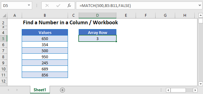
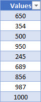
Find a Number in a Column
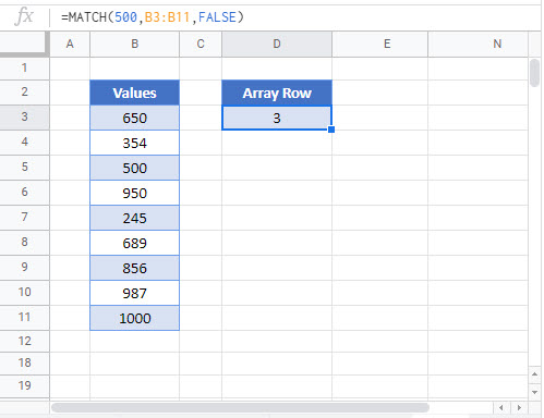
The MATCH Function is useful when you want to find a number within a array of values.
This example will find 500 in column B.
=MATCH(500,B3:B11, 0)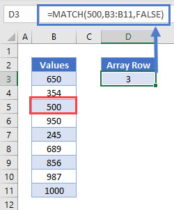
The position of 500 is the 3rd value in the range and returns 3.
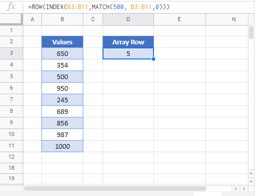
Find Row Number of Value Using ROW, INDEX and MATCH Functions
To find the row number of the value found, we can add the ROW and INDEX functions to the MATCH Function.
=ROW(INDEX(B3:B11,MATCH(987,B3:B11,0)))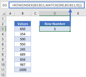
ROW and INDEX Functions
The MATCH Function returns 3 as we have seen from the previous example. The INDEX Function will then return the cell reference or value of the array position returned by the MATCH Function. The ROW function will then return the row of that cell reference.
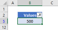
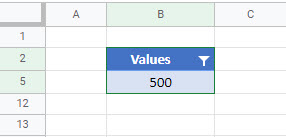
Filter in Excel
We can find a specific number in an array of data by using a Filter in Excel.
- Click in the Range you want to filter ex B3:B10.
- In the Ribbon, select Home > Editing > Sort & Filter > Filter.
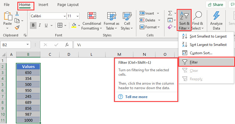
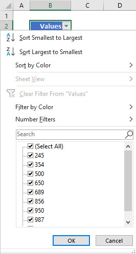
- A drop-down list will be added to the first row in your selected range.
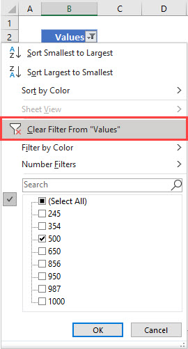
- Click on the drop-down list to get a list of available options.
- Type 500 in the search bar.
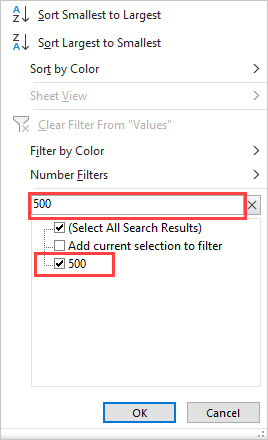
- Click OK.
- If your range has more than one value of 500, then both would show.
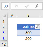
- The rows that do not contain the required values are hidden, and the visible row headers are shown in BLUE.
- To clear the filter, click on the drop-down and then click Clear Filter From “Values”.
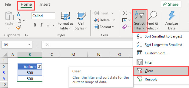
To remove the filter entirely from the Range, select Home > Editing > Sort & Filter > Clear in the Ribbon.
Find Number in Workbook or Worksheet using FIND in Excel
We can look for values in Excel using the FIND functionality.
- In your workbook, press Ctrl+F on the keyboard.
OR
In the Ribbon, select Home > Editing > Find & Select.
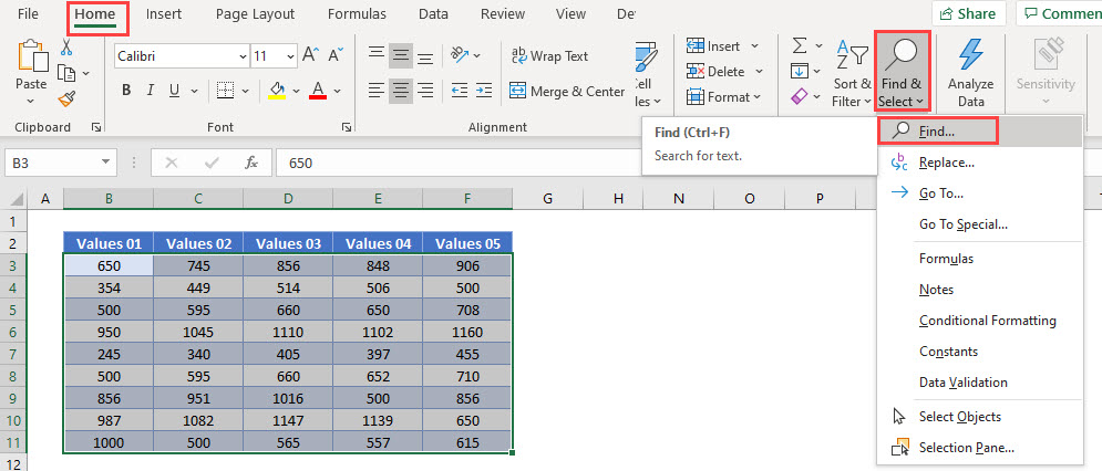
- Type in the value you wish to find.
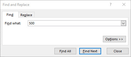
- Click Find Next.
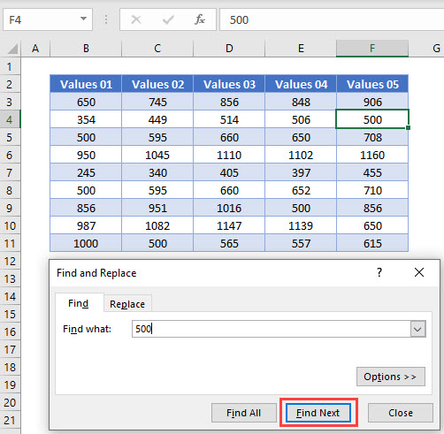
- Continue to click Find Next to move through all the available values in the Worksheet.
- Click Find All to find all the instances of the value in the worksheet.
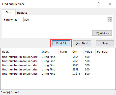
Click Options.
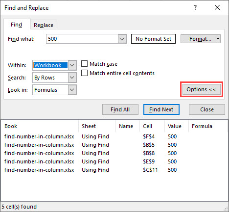
- Amend the Within from Sheet to Workbook and click Find All
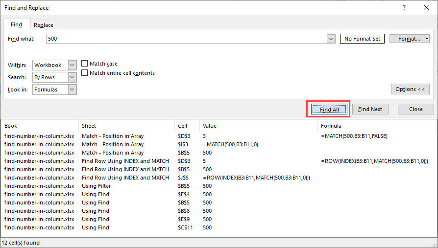
- All the matching values will appear in the results shown.
Find a Number – MATCH Function in Google Sheets
The MATCH Function works the same in Google Sheets as it does in Excel.
Find Row Number of Value Using ROW, INDEX and MATCH Functions in Google Sheets
The ROW, INDEX and MATCH Functions works the same in Google Sheets as it does in Excel.
Filter in Google Sheets
We can find a specific number in an array of data by using Filter in Google Sheets.
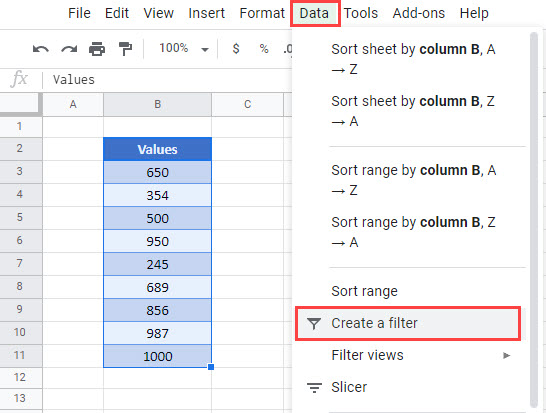
- Click in the Range you want to filter ex B3:B10.
- In the Menu, select Data > Create a filter
- In the Search bar, type in the value you wish to filter on.
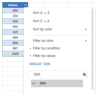
- Click OK.
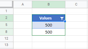
- If your range has more than one value of 500, then both would show.
- The rows that do not contain the required values are hidden.
- To clear the filter, click on the drop-down, click Select All” and then click
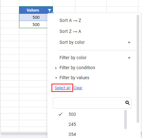
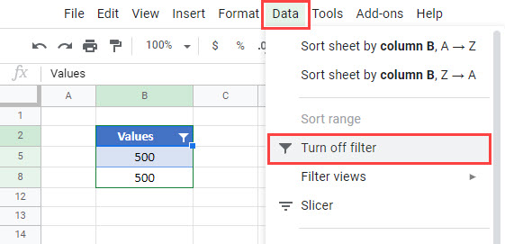
To remove the filter entire, in the Menu, select Data > Turn off Filter.
Find Number in Workbook or Worksheet using FIND in Google Sheets
We can look for values in Google Sheets using the FIND functionality.
- In your workbook, press Ctrl+F on the keyboard.
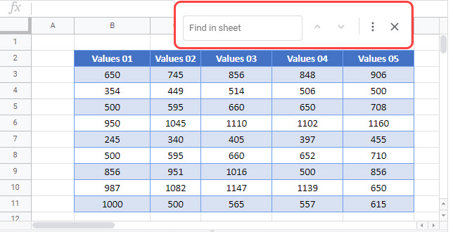
- Type in the value you wish to find.
- All the matching values in the current sheet will be highlighted, with the first one being selected as shown below.
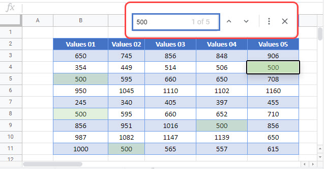
- Select More Options.

- Amend the search to All Sheets.
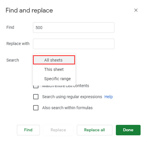
- Click Find.
- The first instance of the value will be found. Click Find again to go to the next value and continue to click Find to find all the matching values in the workbook.
- Click Done to exit out of the Find and Replace Dialog Box.
In this example, the goal is to test the passwords in column B to see if they contain a number. This is a surprisingly tricky problem because Excel doesn’t have a function that will let you test for a number inside a text string directly. Note this is different from checking if a cell value is a number. You can easily perform that test with the ISNUMBER function. In this case, however, we to test if a cell value contains a number, which may occur anywhere. One solution is to use the FIND function with an array constant. In Excel 365, which supports dynamic array formulas, you can use a different formula based on the SEQUENCE function. Both approaches are explained below.
FIND function
The FIND function is designed to look inside a text string for a specific substring. If FIND finds the substring, it returns a position of the substring in the text as a number. If the substring is not found, FIND returns a #VALUE error. For example:
=FIND("p","apple") // returns 2
=FIND("z","apple") // returns #VALUE!
We can use this same idea to check for numbers as well:
=FIND(3,"app637") // returns 5
=FIND(9,"app637") // returns #VALUE!
The challenge in this case is that we need to check the values in column B for ten different numbers, 0-9. One way to do that is to supply these numbers as the array constant {0,1,2,3,4,5,6,7,8,9}. This is the approach taken in the formula in cell D5:
=COUNT(FIND({0,1,2,3,4,5,6,7,8,9},B5))>0Inside the COUNT function, the FIND function is configured to look for all ten numbers in cell B5:
FIND({0,1,2,3,4,5,6,7,8,9},B5)Because we are giving FIND ten values to look for, it returns an array with 10 results. In other words, FIND checks the text in B5 for each number and returns all results at once:
{#VALUE!,4,5,6,#VALUE!,#VALUE!,#VALUE!,#VALUE!,#VALUE!,#VALUE!}Unless you look at arrays often, this may look pretty cryptic. Here is the translation: The number 1 was found at position 4, the number 2 was found at position 5, and the number 3 was found at position 6. All other numbers were not found and returned #VALUE errors.
We are very close now to a final formula. We simply need to tally up results. To do this, we nest the FIND formula above inside the COUNT function like this:
=COUNT(FIND({0,1,2,3,4,5,6,7,8,9},B5))FIND returns the array of results directly to COUNT, which counts the numbers in the array. COUNT only counts numeric values, and ignores errors. This means COUNT will return a number greater than zero if there are any numbers in the value being tested. In the case of cell B5, COUNT returns 3.
The last step is to check the result from COUNT and force a TRUE or FALSE result. We do this by adding «>0» to the end of formula:
=COUNT(FIND({0,1,2,3,4,5,6,7,8,9},B5))>0Now the formula will return TRUE or FALSE. To display a custom result, you can use the IF function:
=IF(COUNT(FIND({0,1,2,3,4,5,6,7,8,9},B5))>0, "Yes", "No")
The original formula is now nested inside IF as the logical_test argument. This formula will return «Yes» if B5 contains a number and «No» if not.
SEQUENCE function
In Excel 365, which offers dynamic array formulas, we can take a different approach to this problem.
=COUNT(--MID(B5,SEQUENCE(LEN(B5)),1))>0This isn’t necessarily a better approach, just a different way to solve the same problem. At the core, this formula uses the MID function together with the SEQUENCE function to split the text in cell B5 into an array:
MID(B5,SEQUENCE(LEN(B5)),1)Working from the inside out, the LEN function returns the length of the text in cell B5:
LEN(B5) // returns 6This number is returned to the SEQUENCE function as the rows argument, and SEQUENCE returns an array of numbers, 1-6:
=SEQUENCE(LEN(B5))
=SEQUENCE(6)
={1;2;3;4;5;6}
This array is returned to the MID function as the start_num argument, and, with num_chars set to 1, the MID function returns an array that contains the characters in cell B5:
=MID(B5,{1;2;3;4;5;6},1)
={"a";"b";"c";"1";"2";"3"}
We can now simplify the original formula to:
=COUNT(--{"a";"b";"c";"1";"2";"3"})>0We use the double-negative (—) to get Excel to try and coerce the values in the array into numbers. The result looks like this:
=COUNT({#VALUE!;#VALUE!;#VALUE!;1;2;3})>0The math operation created by the double negative (—) returns an actual number when successful and a #VALUE! error when the operation fails. The COUNT function counts the numbers, ignoring any errors, and returns 3. As above, we check the final count with «>0», and the result for cell B5 is TRUE.
Note: as you might guess, you can easily adapt this formula to count numbers in a text string.
Cell equals number?
Note that the formulas above are too complex if you only want to test if a cell equals a number. In that case, you can simply use the ISNUMBER function like this:
=ISNUMBER(A1)
Find in Excel (Table of Contents)
- Using Find and Select Feature in Excel
- FIND Function in Excel
- SEARCH Function in Excel
Introduction to Find in Excel
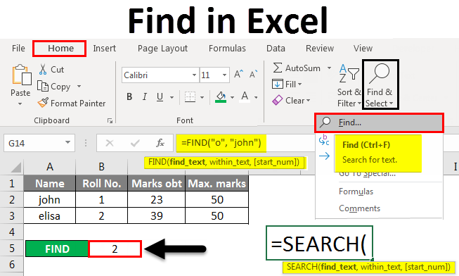
There are two ways to find it in Excel. First, we can use Find by pressing Ctrl + F shortcut keys. Therein Find and Replace box, search the word or field which we want to find in the Find What section. In another way, we can use the FIND function. For this, select the Find function from the insert function and, as per syntax, select the substring from where we need to find it, and choose the word or letter or number which we want to find in the String position. This will return the position of the chosen string from the selected Substring.
Methods to Find in Excel
Below are the different methods to find in excel.
You can download this Find in Excel Template here – Find in Excel Template
Method #1 – Using Find and Select Feature in Excel
Let’s see How to Find a Number or a Character in Excel using the Find and Select feature in Excel.
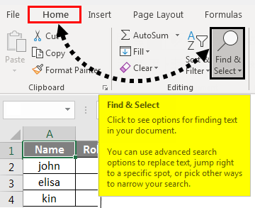
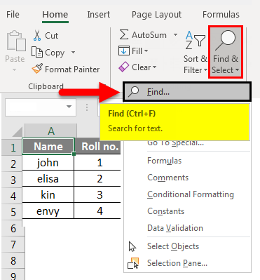
Step 1 – Under the Home tab, in the Editing group, click Find & Select.
Step 2 – To find text or numbers, click Find.
- In the Find what box, type the text or character you want to search for, or click the arrow in the Find what box and then click a recent search in the list.
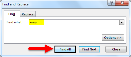
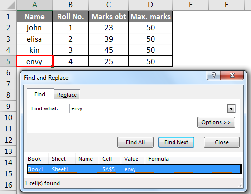
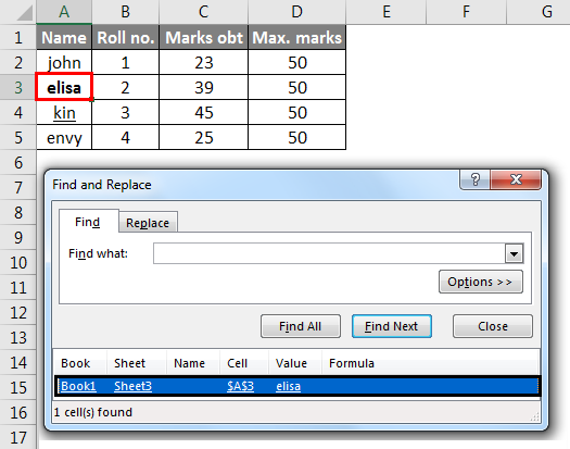
Here, we have a record of marks of four students. Suppose we want to find the text ‘envy’ in this table. For this, we click Find and Select under the Home tab then the Find and Replace dialog box appears. In the Find what box, we enter ‘envy’ then click on Find All. We get the text ‘envy’ is in cell number A5.
- You can use wildcard characters, such as an asterisk (*) or a question mark (?), in your search criteria:
Use the asterisk to find any string of characters.
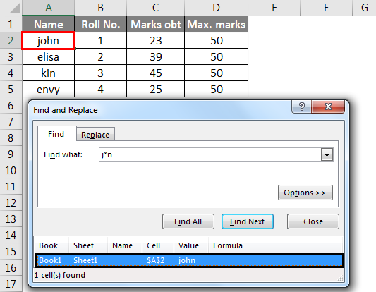
Suppose we want to find text in the table which starts with the letter ‘j’ and ends with the letter ‘n’. In the Find and Replace dialog box, we enter ‘j*n’ in the Find what box, then click on Find All.
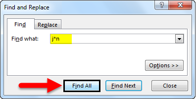
We will get the result as text ‘j*n’(john) is in the cell no. ‘A2’ because we have only one text which starts with ‘j’ and ends with ‘n’ with any number of characters between them.
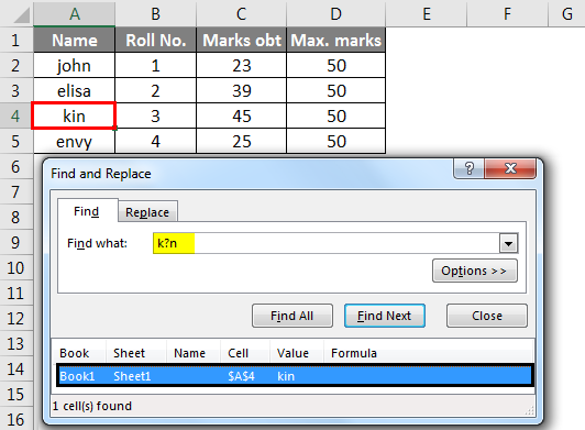
Use the question mark to find any single character.
Suppose we want to find text in the table that starts with the letter ‘k’ and ends with the letter ‘n’ with a single character. So, in the Find and Replace dialog box, we enter ‘k?n’ to find what box. Then click on Find All.
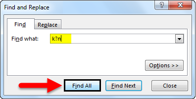
Here, we get the text ‘k?n’(kin) is in cell no. ‘A4’ because we have only one text which starts with ‘k’ and ends with ‘n’ with a single character between them.
- Click Options to further define your search if needed.
- We can find text or number by changing settings in the Within, Search and Look in the box according to our needs.
- To show the working of the above-mentioned options, we took the data as follows.
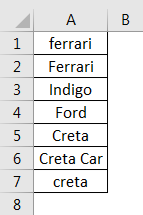
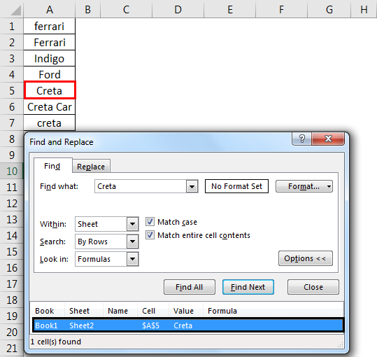
- To search case-sensitive data, select the Match case check box. It gives you output in the case you give input in the Find What box. For example, we have a table of some cars’ names. If you type ‘ferrari’ in the Find What box, then it will find only ‘ferrari’, not ‘Ferrari’.
- To search for cells that contain just the characters you typed in the Find what box, select the Match entire cell contents checkbox. For example, we have a table of some cars’ names. Type ‘Creta’ in the Find What box.
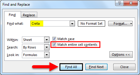
- It will then find cells containing exactly ‘Creta’, and cells containing ‘Cretaa’ or ‘Creta car’ will not be found.
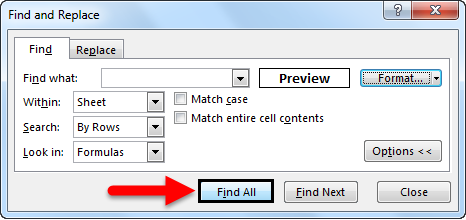
- If you want to search for text or numbers with specific formatting, click Format, and then make your selections in the Find Format dialog box according to your need.
- Let us click the Font option and select the Bold, and click OK.
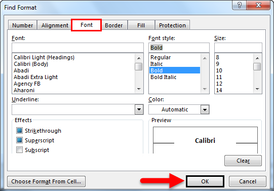
- Then, we click on Find All.
We get the value as ‘elisa’, which is in the ‘A3’ cell.
Method #2 – Using FIND Function in Excel
The FIND function in Excel gives the location of a substring within a string.
Syntax For FIND in Excel:
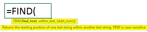
The first two parameters are required, and the last parameter is non-compulsory.
- Find_Value: The substring which you want to find.
- Within_String: The string in which you want to find the specific substring.
- Start_Position: It is a non-compulsory parameter and describes from which position we want to search substring. If you do not describe it, then start the search from the 1st position.
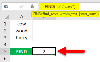
For example =FIND(“o”, “Cow”) gives 2 because “o” is the 2nd letter in the word “cow“.
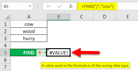
FIND(“j”, “Cow”) gives an error because there is no “j” in “Cow”.
- If the Find_Value parameter contains multiple characters, the FIND function gives the location of the first character.
E.g., the formula FIND(“ur”, “hurry”) gives 2 because “u” in the 2nd letter in the word “hurry”.

- If Within_String contains multiple occurrences of Find_Value, the first occurrence is returned. For example, FIND (“o”, “wood”)
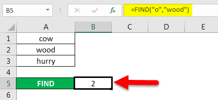
gives 2, which is the location of the first “o” character in the string “wood”.
The Excel FIND function gives the #VALUE! error if:
- If Find_Value does not exist in Within_String.
- If Start_Position contains multiple characters as compared to Within_String.
- If Start_Position either has a zero or negative number.
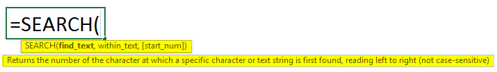
Method #3 – Using SEARCH Function in Excel
The SEARCH function in Excel is simultaneous to FIND because it also gives the location of a substring in a string.
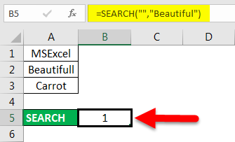
- If Find_Value is the blank string “, the Excel FIND formula gives the string’s first character.
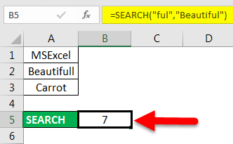
Example =SEARCH (“ful“, “Beautiful) gives 7 because the substring “ful” begins at the 7th position of the substring “beautiful”.
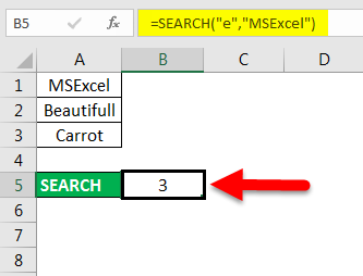
=SEARCH (“e”, “MSExcel”) gives 3 because “e” is the 3rd character in the word “MSExcel” and ignoring the case.
- Excel’s SEARCH function gives the #VALUE! error if:
- If the value of the Find_Value parameter is not found.
- If the Start_Position parameter is superior to the length of Within_String.
- If the Start_Position either equal to or less than 0.
Things to Remember About Find in Excel
- Asterisk defines a string of characters, and the question mark defines a single character. You can also find asterisks, question marks, and tilde characters (~) in worksheet data by preceding them with a tilde character inside the Find what option.
For example, to find data that contain “*”, you would type ~* as your search criteria.
- If you want to find cells that match a specific format, you can delete any criteria in the Find what box and select a specific cell format as an example. Click the arrow next to Format, click Choose Format From Cell, and click the cell with the formatting you want to search for.
- MSExcel saves the formatting options you define; you should clear the formatting options from the last search by clicking on an arrow next to Format and then Clear Find Format.
- The FIND function is case sensitive and does not allow while using wildcard characters.
- The SEARCH function is case-insensitive and allows while using wildcard characters.
Recommended Articles
This is a guide to Find in Excel. Here we discuss how to use the Find feature, Formula for FIND, and SEARCH in Excel, along with practical examples and a downloadable excel template. You can also go through our other suggested articles –
- FIND Function in Excel
- Excel SEARCH Function
- Find and Replace in Excel
- Search For Text in Excel