
![]()
Download Article
![]()
Download Article
Need to find the sum of a column, row, or set of numbers in Excel? Microsoft Excel comes with many mathematical functions, including multiple ways to add sets of numbers. This wikiHow article will teach you the easiest ways to add numbers, cell values, and ranges in Microsoft Excel.
-

1
Click the cell in which you want to display the sum.
-
2
Type an equal sign =. This indicates the beginning of a formula.
Advertisement
-
3
Type the first number you want to add. If you would rather add the value of an existing cell instead of typing a number manually, just click the cell you want to include in the equation. Otherwise, you can type a number manually.
- For example, if you click cell C3, the value of C3 will be the first number in your equation. If you type 1, the number 1 will be the first number in your equation.
-
4
Type a + sign.
-
5
Type another number select another cell. This adds the second number or value to your equation.
- You can add multiple cells or numbers at once if you’d like—just separate each number or address with another + sign.[1]
- For example, if you want to find the sum of cells C3, D4, and E5, your formula will look like this =C3+D4+E5.
- If you want to add 1 plus 1, your formula will look like this: =1+1 .
- You can add other operations, such as subtraction or multiplication, in the same equation. In this example, we’ll add the values of C3 and D4 and then subtract 2: =C3+D4-2
- You can add multiple cells or numbers at once if you’d like—just separate each number or address with another + sign.[1]
-
6
Press ↵ Enter or ⏎ Return. Now you’ll see the sum of the added numbers or values in the selected cell.


Advertisement
-
1
Click the cell in which you want to display the sum. The SUM function works like using the plus + sign, but is a bit easier to work with when you’re adding multiple cells and ranges.
-
2
Type an equal sign followed by the word SUM =SUM. This indicates the beginning of the SUM formula.
-
3
Type an opening parenthesis (. Your formula should now look like this: =SUM(.
-
4
Select the range of cells you want to add. Click and drag over all of the cells you want to add together. For example, if you want to add the values of all cells from A1 through A10, select all of those cells now.
- You can also select multiple columns and rows here. To select multiple non-adjacent columns and/or rows, hold down the Control key and as you select each range.
- You don’t have to select entire ranges with the SUM function—you can also enter individual numbers or cell addresses.
-
5
Type a clothing parenthesis ). This finishes the formula.
- Your formula should now look something like this: =SUM(B4,B8)
- In this example, we’ve selected cells B4 through B8
- If you selected non-adjacent ranges, each range will be separated by a comma. In this example, we selected B4 through C8 (two adjacent columns) and E4 through E5: =SUM(B4:C8,E4:E5)
- Your formula should now look something like this: =SUM(B4,B8)
-
6
Press ↵ Enter or ⏎ Return. The sum of the selected range now appears in this cell.


Advertisement
-
1
Click the cell immediately below or next to the values you want to add. AutoSum will automatically create a formula that adds the values of an adjacent column or row.[2]
- For example, if you want to add the values of cells A:2 through A:10, you would click cell A11.
- You can also add multiple columns or rows at the same time by selecting multiple cells. For example, to display the sums of values in columns A, B, and C, you could select cells A11, B11, and C11.
-
2
Click the AutoSum icon on the Home tab Σ. It’s the Sigma icon (which looks like an «E») on the Home tab at the top of Excel. A formula will then appear in the selected cell.
-
3
Press ↵ Enter or ⏎ Return. Now you’ll see the results of the formula in the cell.
- If you selected multiple blank cells, you’ll see each individual column or row’s value in the selected cells.


Advertisement
Ask a Question
200 characters left
Include your email address to get a message when this question is answered.
Submit
Advertisement
-
Use the SUMIF function to add cells that match certain criteria. For example, if you wanted to find the sum of all cells in A2 through A:10 that are greater than 1, you’d use =SUMIF(A2:A10, ">1").[3]
Thanks for submitting a tip for review!
Advertisement
About This Article
Article SummaryX
1. Use a plus sign to write out formulas like this: =4+5
2. Use the SUM formula to add values from one or more ranges.
3. Use AUTOSUM to automatically find the total of a column or row.
Did this summary help you?
Thanks to all authors for creating a page that has been read 108,680 times.
Is this article up to date?
Excel for Microsoft 365 Excel for Microsoft 365 for Mac Excel for the web Excel 2021 Excel 2021 for Mac Excel 2019 Excel 2019 for Mac Excel 2016 Excel 2016 for Mac Excel 2013 Excel 2010 Excel 2007 More…Less
Although Excel includes a multitude of built-in worksheet functions, chances are it doesn’t have a function for every type of calculation you perform. The designers of Excel couldn’t possibly anticipate every user’s calculation needs. Instead, Excel provides you with the ability to create custom functions, which are explained in this article.
Custom functions, like macros, use the Visual Basic for Applications (VBA) programming language. They differ from macros in two significant ways. First, they use Function procedures instead of Sub procedures. That is, they start with a Function statement instead of a Sub statement and end with End Function instead of End Sub. Second, they perform calculations instead of taking actions. Certain kinds of statements, such as statements that select and format ranges, are excluded from custom functions. In this article, you’ll learn how to create and use custom functions. To create functions and macros, you work with the Visual Basic Editor (VBE), which opens in a new window separate from Excel.
Suppose your company offers a quantity discount of 10 percent on the sale of a product, provided the order is for more than 100 units. In the following paragraphs, we’ll demonstrate a function to calculate this discount.
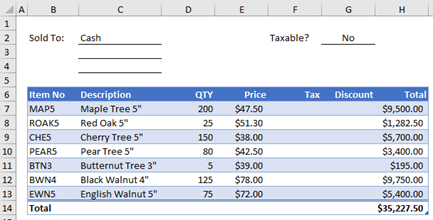
The example below shows an order form that lists each item, quantity, price, discount (if any), and the resulting extended price.
To create a custom DISCOUNT function in this workbook, follow these steps:
-
Press Alt+F11 to open the Visual Basic Editor (on the Mac, press FN+ALT+F11), and then click Insert > Module. A new module window appears on the right-hand side of the Visual Basic Editor.
-
Copy and paste the following code to the new module.
Function DISCOUNT(quantity, price)
   If quantity >=100 Then
     DISCOUNT = quantity * price * 0.1
   Else
     DISCOUNT = 0
   End If

 DISCOUNT = Application.Round(Discount, 2)
End Function
Note: To make your code more readable, you can use the Tab key to indent lines. The indentation is for your benefit only, and is optional, as the code will run with or without it. After you type an indented line, the Visual Basic Editor assumes your next line will be similarly indented. To move out (that is, to the left) one tab character, press Shift+Tab.
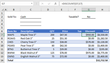
Now you’re ready to use the new DISCOUNT function. Close the Visual Basic Editor, select cell G7, and type the following:
=DISCOUNT(D7,E7)
Excel calculates the 10 percent discount on 200 units at $47.50 per unit and returns $950.00.
In the first line of your VBA code, Function DISCOUNT(quantity, price), you indicated that the DISCOUNT function requires two arguments, quantity and price. When you call the function in a worksheet cell, you must include those two arguments. In the formula =DISCOUNT(D7,E7), D7 is the quantity argument, and E7 is the price argument. Now you can copy the DISCOUNT formula to G8:G13 to get the results shown below.
Let’s consider how Excel interprets this function procedure. When you press Enter, Excel looks for the name DISCOUNT in the current workbook and finds that it is a custom function in a VBA module. The argument names enclosed in parentheses, quantity and price, are placeholders for the values on which the calculation of the discount is based.
The If statement in the following block of code examines the quantity argument and determines whether the number of items sold is greater than or equal to 100:
If quantity >= 100 Then
 DISCOUNT = quantity * price * 0.1
Else
 DISCOUNT = 0
End If
If the number of items sold is greater than or equal to 100, VBA executes the following statement, which multiplies the quantity value by the price value and then multiplies the result by 0.1:
Discount = quantity * price * 0.1
The result is stored as the variable Discount. A VBA statement that stores a value in a variable is called an assignment statement, because it evaluates the expression on the right side of the equal sign and assigns the result to the variable name on the left. Because the variable Discount has the same name as the function procedure, the value stored in the variable is returned to the worksheet formula that called the DISCOUNT function.
If quantity is less than 100, VBA executes the following statement:
Discount = 0
Finally, the following statement rounds the value assigned to the Discount variable to two decimal places:
Discount = Application.Round(Discount, 2)
VBA has no ROUND function, but Excel does. Therefore, to use ROUND in this statement, you tell VBA to look for the Round method (function) in the Application object (Excel). You do that by adding the word Application before the word Round. Use this syntax whenever you need to access an Excel function from a VBA module.
A custom function must start with a Function statement and end with an End Function statement. In addition to the function name, the Function statement usually specifies one or more arguments. You can, however, create a function with no arguments. Excel includes several built-in functions—RAND and NOW, for example—that don’t use arguments.
Following the Function statement, a function procedure includes one or more VBA statements that make decisions and perform calculations using the arguments passed to the function. Finally, somewhere in the function procedure, you must include a statement that assigns a value to a variable with the same name as the function. This value is returned to the formula that calls the function.
The number of VBA keywords you can use in custom functions is smaller than the number you can use in macros. Custom functions are not allowed to do anything other than return a value to a formula in a worksheet, or to an expression used in another VBA macro or function. For example, custom functions cannot resize windows, edit a formula in a cell, or change the font, color, or pattern options for the text in a cell. If you include “action” code of this kind in a function procedure, the function returns the #VALUE! error.
The one action a function procedure can do (apart from performing calculations) is display a dialog box. You can use an InputBox statement in a custom function as a means of getting input from the user executing the function. You can use a MsgBox statement as a means of conveying information to the user. You can also use custom dialog boxes, or UserForms, but that’s a subject beyond the scope of this introduction.
Even simple macros and custom functions can be difficult to read. You can make them easier to understand by typing explanatory text in the form of comments. You add comments by preceding the explanatory text with an apostrophe. For example, the following example shows the DISCOUNT function with comments. Adding comments like these makes it easier for you or others to maintain your VBA code as time passes. If you need to make a change to the code in the future, you’ll have an easier time understanding what you did originally.
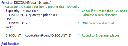
An apostrophe tells Excel to ignore everything to the right on the same line, so you can create comments either on lines by themselves or on the right side of lines containing VBA code. You might begin a relatively long block of code with a comment that explains its overall purpose and then use inline comments to document individual statements.
Another way to document your macros and custom functions is to give them descriptive names. For example, rather than name a macro Labels, you could name it MonthLabels to describe more specifically the purpose the macro serves. Using descriptive names for macros and custom functions is especially helpful when you’ve created many procedures, particularly if you create procedures that have similar but not identical purposes.
How you document your macros and custom functions is a matter of personal preference. What’s important is to adopt some method of documentation, and use it consistently.
To use a custom function, the workbook containing the module in which you created the function must be open. If that workbook is not open, you get a #NAME? error when you try to use the function. If you reference the function in a different workbook, you must precede the function name with the name of the workbook in which the function resides. For example, if you create a function called DISCOUNT in a workbook called Personal.xlsb and you call that function from another workbook, you must type =personal.xlsb!discount(), not simply =discount().
You can save yourself some keystrokes (and possible typing errors) by selecting your custom functions from the Insert Function dialog box. Your custom functions appear in the User Defined category:
An easier way to make your custom functions available at all times is to store them in a separate workbook and then save that workbook as an add-in. You can then make the add-in available whenever you run Excel. Here’s how to do this:
-
After you have created the functions you need, click File > Save As.
In Excel 2007, click the Microsoft Office Button, and click Save As
-
In the Save As dialog box, open the Save As Type drop-down list, and select Excel Add-In. Save the workbook under a recognizable name, such as MyFunctions, in the AddIns folder. The Save As dialog box will propose that folder, so all you need to do is accept the default location.
-
After you have saved the workbook, click File > Excel Options.
In Excel 2007, click the Microsoft Office Button, and click Excel Options.
-
In the Excel Options dialog box, click the Add-Ins category.
-
In the Manage drop-down list, select Excel Add-Ins. Then click the Go button.
-
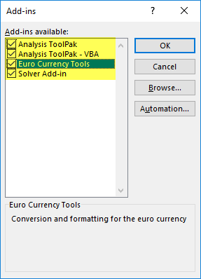
In the Add-Ins dialog box, select the check box beside the name you used to save your workbook, as shown below.
-
After you have created the functions you need, click File > Save As.
-
In the Save As dialog box, open the Save As Type drop-down list, and select Excel Add-In. Save the workbook under a recognizable name, such as MyFunctions.
-
After you have saved the workbook, click Tools > Excel Add-Ins.
-
In the Add-Ins dialog box, select the Browse button to find your add-in, click Open, then check the box beside your Add-In in the Add-Ins Available box.
After you follow these steps, your custom functions will be available each time you run Excel. If you want to add to your function library, return to the Visual Basic Editor. If you look in the Visual Basic Editor Project Explorer under a VBAProject heading, you will see a module named after your add-in file. Your add-in will have the extension .xlam.
Double-clicking that module in the Project Explorer causes the Visual Basic Editor to display your function code. To add a new function, position your insertion point after the End Function statement that terminates the last function in the Code window, and begin typing. You can create as many functions as you need in this manner, and they will always be available in the User Defined category in the Insert Function dialog box.
This content was originally authored by Mark Dodge and Craig Stinson as part of their book Microsoft Office Excel 2007 Inside Out. It has since been updated to apply to newer versions of Excel as well.
Need more help?
You can always ask an expert in the Excel Tech Community or get support in the Answers community.
Need more help?
Want more options?
Explore subscription benefits, browse training courses, learn how to secure your device, and more.
Communities help you ask and answer questions, give feedback, and hear from experts with rich knowledge.
What are Add-ins in Excel?
An add-ins is an extension that adds more features and options to Microsoft Excel. Providing additional functions to the user increases the power of Excel. An add-in needs to be enabled for usage. Once enabled, it activates as Excel is started.
For example, Excel add-ins can perform tasks like creating, deleting, and updating the data of a workbook. Moreover, one can add buttons to the Excel ribbon and run custom functions with add-ins.
The Solver, Data Analysis (Analysis ToolPakExcel’s data analysis toolpak can be used by users to perform data analysis and other important calculations. It can be manually enabled from the addins section of the files tab by clicking on manage addins, and then checking analysis toolpak.read more), and Analysis ToolPak-VBA are some essential add-ins.
The purposes of activating add-ins are listed as follows: –
- To interact with the objects of Excel
- To avail an extended range of functions and buttons
- To facilitate the setting up of standard add-ins throughout an organization
- To serve the varied needs of a broad audience
In Excel, one can access several Add-ins from “Add-ins” under the “Options” button of the “File” tab. In addition, one can select from the drop-down “Manage” in the “Add-ins” window for more add-ins.
By default, it might hide some add-ins. One can view the unhidden add-ins in the “Data” tab on the Excel ribbonThe ribbon is an element of the UI (User Interface) which is seen as a strip that consists of buttons or tabs; it is available at the top of the excel sheet. This option was first introduced in the Microsoft Excel 2007.read more. For example, it is shown in the following image.
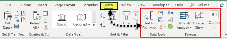
Table of contents
- What are Add-ins in Excel?
- How to Install Add-ins in Excel?
- Types of Add-ins in Excel
- The Data Analysis Add-in
- Create Custom Functions and Install as an Excel Add-in
- Example #1–Extract Comments from the Cells of Excel
- Example #2–Hide Worksheets in Excel
- Example #3–Unhide the Hidden Sheets of Excel
- The Cautions While Creating Add-ins
- Frequently Asked Questions
- Recommended Articles
How to Install Add-ins in Excel?
If Excel is not displaying the add-ins, they need to be installed. The steps to install Excel add-ins are listed as follows:
- First, click on the “File” tab located at the top left corner of Excel.

- Click “Options,” as shown in the following image.

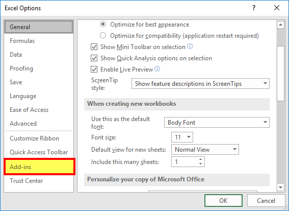
- The “Excel Options” window opens. Select “Add-ins.”

- There is a box to the right of “Manage” at the bottom. Click the arrow to view the drop-down menu. Select “Excel add-ins” and click “Go.”

- The “Add-ins” dialog box appears. Select the required checkboxes and click “OK.” We have selected all four add-ins.

- The “Data Analysis” and “Solver” options appear under the “Data tab” of the Excel ribbon.


Types of Add-ins in Excel
The types of add-ins are listed as follows:
- Inbuilt add-ins: These are built into the system. One can unhide them by performing the steps listed under the preceding heading (how to install add-ins in Excel?).
- Downloadable add-ins: These can be downloaded from the Microsoft website (www.office.com).
- Custom add-ins: These are designed to support the basic functionality of Excel. They may be free or chargeable.
The Data Analysis Add-in
The “Data Analysis Tools” pack analyzes statistics, finance, and engineering data.

The various tools available under the “Data Analysis” add-in are shown in the following image.

Create Custom Functions and Install them as an Excel Add-in
Generally, an add-in is created with the help of VBA macrosVBA Macros are the lines of code that instruct the excel to do specific tasks, i.e., once the code is written in Visual Basic Editor (VBE), the user can quickly execute the same task at any time in the workbook. It thus eliminates the repetitive, monotonous tasks and automates the process.read more. Let us learn to create an add-in (in all Excel files) for a custom functionCustom Functions, also known as UDF (User Defined Functions) in Excel, are personalized functions that the users create through VBA programming code to fulfill their particular requirements. read more. For this, first, we make a custom function.
Let us consider some examples.
You can download this Excel Add-Ins Excel Template here – Excel Add-Ins Excel Template
We want to extract comments from specific cells of Excel. Then, create an add-in for the same.
The steps for creating an add-in and extracting comments from cells are listed as follows:
Step 1: Open a new workbook.
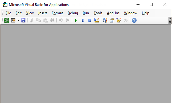
Step 2: Press the shortcutAn Excel shortcut is a technique of performing a manual task in a quicker way.read more “ALT+F11” to access the “Visual Basic Editor.” The following image shows the main screen of Microsoft Visual Basic for Applications.
Step 3: Click “Module” under the “Insert” tab, shown in the following image.

Step 4: Enter the following code in the “module” window.
Function TakeOutComment(CommentCell As Range) As String
TakeOutComment = CommentCell.Comment.Text
End Function

Step 5: Once the code is entered, save the file with the type “Excel add-in.”

Step 6: Open the file containing comments.
Step 7: Select ” Options ” in the “File” tab and select “Options.” Choose “Add-ins.” In the box to the right of “Manage,” select “Excel Add-ins.” Click “Go.”
Click the “Browse” option in the “Add-ins” dialog box.

Step 8: Select the add-in file that had been saved. Click “Ok.”
We saved the file with the name “Excel Add-in.”

Step 9: The workbook’s name (Excel Add-in) that we had saved appears as an add-in, as shown in the following image.
This add-in can be applied as an Excel formula to extract comments.

Step 10: Go to the sheet containing comments. The names of three cities appear with comments, as shown in the following image.

Step 11: In cell B1, enter the symbol “equal to” followed by the function’s name. Type “TakeOutComment,” as shown in the following image.

Step 12: Select cell A1 as the reference. It extracts the comment from the mentioned cell.
Since there are no comments in cells A2 and A3, the formula returns “#VALUE!.”

Example #2–Hide Worksheets in Excel
We want to hide Excel worksheets except for the active sheet. Create an add-in and icon on the Excel toolbar for the same.
The steps to hide worksheets (except for the currently active sheet) and, after that, create an add-in and icon are listed as follows:
Step 1: Open a new workbook.
Step 2: In the “Visual Basic” window, insert a “Module” from the Insert tab. The same is shown in the following image.
Step 3: Copy and paste the following code into the module.
Sub Hide_All_Worksheets_()
Dim As Worksheet
For Each Ws In ActiveWorkbook.Worksheets
If Ws.Name <> ActiveSheet.Name Then
Ws.Visible = xlSheetVeryHidden
End If
Next Ws
End Sub

Step 4: Save this workbook with the type “Excel add-in.”
Step 5: Add this add-in to the new workbook. For this, click “Options” under the “File” tab. Select “Add-ins.” In the box to the right of “Manage,” select “Excel add-in” Click “Go.”
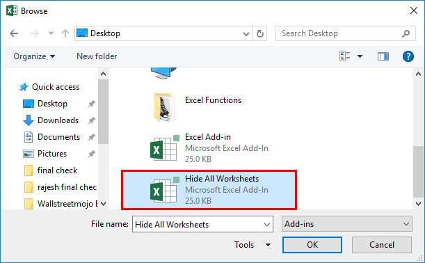
In the “Add-ins” window, choose “Browse.”

Step 6: Select the saved add-in file. Click “Ok.”
We have saved the file with the name “Hide All Worksheets.”
Step 7: The new add-in “Hide All Worksheets” appears in the “Add-ins” window.

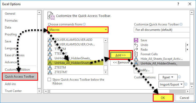
Step 8: Right-click the Excel ribbon and select “Customize the Ribbon.”

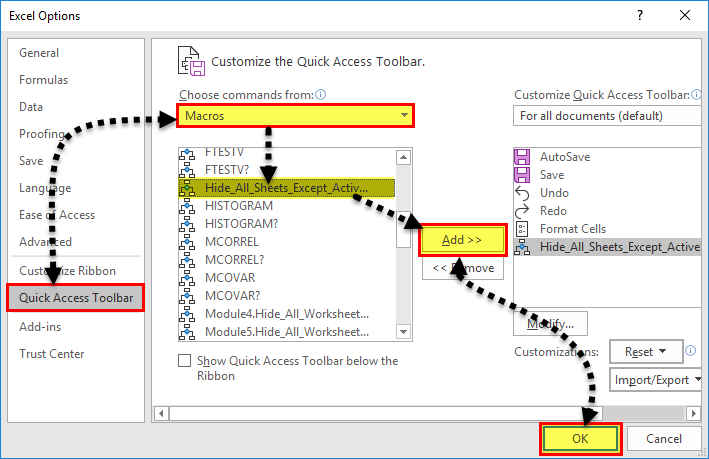
Step 9: The “Excel Options” window appears. Click “Quick Access Toolbar.” Under the drop-down of “Choose commands from,” select “macrosA macro in excel is a series of instructions in the form of code that helps automate manual tasks, thereby saving time. Excel executes those instructions in a step-by-step manner on the given data. For example, it can be used to automate repetitive tasks such as summation, cell formatting, information copying, etc. thereby rapidly replacing repetitious operations with a few clicks.
read more.”
In the box following this drop-down, choose the name of the macro. Then, click “Add” followed by “OK.” The tasks of this step are shown with the help of black arrows in the following image.
Step 10: A small icon appears on the toolbar. Clicking this icon hides all worksheets except for the currently active sheet.

Example #3–Unhide the Hidden Sheets of Excel
If we want to unhide the sheetsThere are different methods to Unhide Sheets in Excel as per the need to unhide all, all except one, multiple, or a particular worksheet. You can use Right Click, Excel Shortcut Key, or write a VBA code in Excel. read more hidden in the preceding example (example #2). Create an add-in and toolbar icon for the same.
The steps to unhide the sheets and, after that, create an add-in and toolbar icon are listed as follows:
Step 1: Copy and paste the following code to the “Module” inserted in Microsoft Visual Basic for Applications.
Sub UnHide_All_HiddenSheets_()
Dim Ws As Worksheet
For Each Ws In ActiveWorkbook.Worksheets
Ws.Visible = xlSheetVisible
Next Ws
End Sub

Step 2: Save the file as “Excel add-in.” Add this add-in to the sheet.
Right-click the Excel ribbon and choose the option “Customize the ribbon.” Then, in the “Quick Access Toolbar,” select “Macros” under the drop-down of “Choose commands from.”
Choose the macro’s name, click “Add” and “OK.” The tasks of this step are shown with the help of black arrows in the following image.
Step 3: Another icon appears on the toolbar. Clicking this icon unhides the hidden worksheets.

The Cautions While Creating Add-ins
The points to be observed while working with add-ins are listed as follows:
- First, remember to save the file in Excel’s “Add-in” extensionExcel extensions represent the file format. It helps the user to save different types of excel files in various formats. For instance, .xlsx is used for simple data, and XLSM is used to store the VBA code.read more of Excel.
- Be careful while selecting the add-ins to be inserted by browsing in the “Add-ins” window.
Note: It is possible to uninstall the unnecessary add-ins at any time.
Frequently Asked Questions
1. What is an add-in? where is it in Excel?
An add-in extends the functions of Excel. It provides more features to the user. It is also possible to create custom functions and insert them as an add-in in Excel.
An add-in can be created, used, and shared with an audience. One can find the add-ins in the “Add-ins” window of Excel.
The steps to access the add-ins in Excel are listed as follows:
a. Click “Options” in the “File” tab of Excel. Select “Add-ins.”
b. In the box to the right of “Manage,” select “Excel add-ins.” Click “Go.”
c. The “Add-ins” window opens. Click “Browse.”
d. Select the required add-in file and click “OK.”
Note: The add-ins already present in the system can be accessed by browsing. Select the corresponding checkbox in the “Add-ins” window and click “OK” to activate an add-in.
2. How to remove an Add-in from Excel?
For removing an add-in from the Excel ribbon, it needs to be inactivated. The steps to inactivate an add-in of Excel are listed as follows:
a. In the File tab, click “Options” and choose “Add-ins”.
b. From the drop-down menu of the “Manage” box, select “Excel add-ins.” Click “Go.”c.
c. In the “Add-ins” window, deselect the checkboxes of the add-ins to be inactivated. Click “OK.”
The deselected add-ins are inactivated. Sometimes, one may need to restart Excel after inactivation. It helps remove the add-in from the ribbon.
Note: Inactivation does not remove an add-in from the computer. For removing an inactivated add-in from the computer, it needs to be uninstalled.
3. How to add an Add-in to the Excel toolbar?
The steps to add an Add-in to the Excel toolbar are listed as follows:
a. In an Excel workbook, press “Alt+F11” to open the Visual Basic Editor. Enter the code by inserting a “module.”
b. Press “Alt+F11” to return to Excel. Save the file as “Excel add-in” (.xlam).
c. In File, select “Options” followed by “Add-ins.” Select “Excel add-ins” in the “Manage” box and click “Go.”
d. Browse this file in the “Add-ins” window. Select the required checkbox and click “OK.”
e. Right-click the ribbon and choose “Customize the Ribbon.” Click “Quick Access Toolbar.”
f. Select “Macros” from the drop-down of “Choose commands from.”
g. Choose the required macro, click “Add” and” OK.”
The icon appears on the toolbar. This icon works in all Excel workbooks as the add-in has been enabled.
Recommended Articles
This article is a step-by-step guide to creating, installing, and using add-ins in Excel. Here, we also discuss the types of Excel add-ins and create a custom function. Take a look at these useful functions of Excel: –
- What is the Quick Access Toolbar in Excel?
- “Save As” Shortcut in Excel
- Remove Duplicates in Excel
- How to Show Formula in Excel?
An Excel add-in can be really useful when you have to run a macro often in different workbooks.
For example, suppose you want to highlight all the cells that have an error in it, you can easily create an Excel add-in that will highlight errors with a click of a button.
Something as shown below (the macro has been added to the Quick Access Toolbar to run it with a single click):

Similarly, you may want to create a custom Excel function and use it in all the Excel workbooks, instead of copy pasting the code again and again.
If you’re interested in learning VBA the easy way, check out my Online Excel VBA Training.
Creating an Excel Add-in
In this tutorial, you’ll learn how to create an Excel add-in. There are three steps to create an add-in and make it available in the QAT.
- Write/Record the code in a module.
- Save as an Excel Add-in.
- Add the macro to the Quick Access Toolbar.
Write/Record the Code in a Module
In this example, we will use a simple code to highlight all the cells that have error values:
Sub HighlightErrors()
 Selection.SpecialCells(xlCellTypeFormulas, xlErrors).Select
 Selection.Interior.Color = vbRed
End Sub
If you are writing code (or copy-pasting it from somewhere), here are steps:
Note: If you are recording a macro, Excel automatically takes care of inserting a module and putting the code in it.
Now let’s go ahead and create an add-in out of this code.
Save and Install the Add-in
Follow the below steps when you are in the workbook where you have inserted the code.
Now the add-in has been activated.
You may not see any tab or option appear in the ribbon, but the add-in gets activated at this stage and the code is available to be used now.
The next step is to add the macro to the Quick Access Toolbar so that you can run the macro with a single click.
Note: If you are creating an add-in that has a custom function, then you don’t need to go to step 3. By the end of step 2, you’ll have the function available in all the workbook. Step 3 is for such codes, where you want something to happen when you run the code (such as highlight cells with errors).
Save and Install the Add-in
To do this:
Now to run this code in any workbook, select the dataset and click on the macro icon in the QAT.
This will highlight all the cells with errors in red color. You can also use this macro in any workbook since you have enabled the add-in.
Caution: The changes done by the macro can’t be undone using Control + Z.
You can also create custom functions and then save it as an Excel add-in. Now, when you enable the add-in, the custom functions would be available in all your Excel workbooks.
You May Also Like the Following Excel Tutorials:
- Working with Cells and Ranges in Excel VBA.
- Working with Worksheets in VBA.
- Working with Workbooks in VBA.
- Using Loops in Excel VBA.
- Using IF Then Else Statement in Excel VBA.
- How to Create and Use Personal Macro Workbook in Excel.
- Useful Excel Macro Code Examples.
- Using For Next Loop in Excel VBA.
- Excel VBA Events – An Easy (and Complete) Guide.
- Excel VBA Error Handling
- Free Courses
- Microsoft Excel
- Insert a Function in Excel

How to Insert Functions in Excel
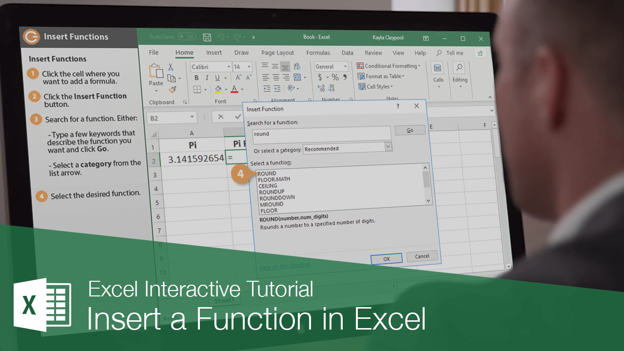
Excel has over 450 functions you can use to perform just about any kind of calculation. If you’re having trouble finding the right function, the Insert Function command lets you search for the function you want. It also guides you through inserting the arguments, which is helpful for complex functions.
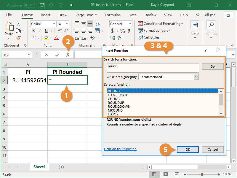
- Click the cell where you want to add a formula.
- Click the Insert Function button.
- Search for a function using one of these methods:
- Type a few keywords that describe the function you want and click Go.
- Select a category from the list arrow menu.
- Select the desired function.
- Click OK.

The Function Arguments dialog box appears. Here you need to specify the arguments for the function you selected. In Excel, an argument can be a range of data, a specified output, or other parameters.
If you’re ever confused about what an argument is, just check the description down here.
- Enter the formula arguments.
- Click OK.
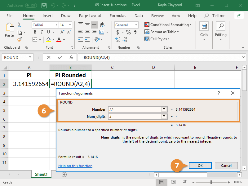
The dialog box closes and Excel displays the results of the inserted formula.

FREE Quick Reference
Click to Download
Free to distribute with our compliments; we hope you will consider our paid training.