Function that returns an array in excel - Word и Excel - помощь в работе с программами

In September, 2018 we announced that Dynamic Array support would be coming to Excel. This allows formulas to spill across multiple cells if the formula returns multi-cell ranges or arrays. This new dynamic array behavior can also affect earlier functions that have the ability to return a multi-cell range or array.

Below is a list of functions that could return multi-cell ranges or arrays in what we refer to as pre-dynamic array Excel. If these functions were used in workbooks predating dynamic arrays, and returned a multi-cell range or array to the grid (or a function that did not expect them), then silent implicit intersection would have occurred. Dynamic array Excel indicates where implicit intersection could occur using the @ operator, and as a result, these functions may be prepended with an @ if they were originally authored in a pre-dynamic array version of Excel. Additionally, if authored on dynamic array Excel, these functions may appear as legacy array formulas in pre-dynamic array Excel unless prepended with @.

CELL
COLUMN
FILTERXML
FORMULATEXT
FREQUENCY
GROWTH
HYPERLINK
INDEX
INDIRECT
ISFORMULA
LINEST
LOGEST
MINVERSE
MMULT
MODE.MULT
MUNIT
OFFSET
ROW
TRANSPOSE
TREND
All User Defined Functions

Need more help?

You can always ask an expert in the Excel Tech Community or get support in the Answers community.

Need more help?

Want more options?

Explore subscription benefits, browse training courses, learn how to secure your device, and more.

Communities help you ask and answer questions, give feedback, and hear from experts with rich knowledge.

Источник

I think Collection might be what you are looking for.

Example:

Private Function getProducts(ByVal supplier As String) As Collection
    Dim getProducts_ As New Collection

    If supplier = "ACME" Then
        getProducts_.Add ("Anvil")
        getProducts_.Add ("Earthquake Pills")
        getProducts_.Add ("Dehydrated Boulders")
        getProducts_.Add ("Disintegrating Pistol")
    End If

    Set getProducts = getProducts_
    Set getProducts_ = Nothing
End Function

Private Sub fillProducts()
    Dim products As Collection
    Set products = getProducts("ACME")
    For i = 1 To products.Count
        Sheets(1).Cells(i, 1).Value = products(i)
    Next i
End Sub

Edit:
Here is a pretty simple solution to the Problem: Populating a ComboBox for Products whenever the ComboBox for Suppliers changes it’s value with as little vba as possible.

Public Function getProducts(ByVal supplier As String) As Collection
    Dim getProducts_ As New Collection
    Dim numRows As Long
    Dim colProduct As Integer
    Dim colSupplier As Integer
    colProduct = 1
    colSupplier = 2

    numRows = Sheets(1).Cells(1, colProduct).CurrentRegion.Rows.Count

    For Each Row In Sheets(1).Range(Sheets(1).Cells(1, colProduct), Sheets(1).Cells(numRows, colSupplier)).Rows
        If supplier = Row.Cells(1, colSupplier) Then
            getProducts_.Add (Row.Cells(1, colProduct))
        End If
    Next Row

    Set getProducts = getProducts_
    Set getProducts_ = Nothing
End Function

Private Sub comboSupplier_Change()
    comboProducts.Clear
    For Each Product In getProducts(comboSupplier)
        comboProducts.AddItem (Product)
    Next Product
End Sub

Notes: I named the ComboBox for Suppliers comboSupplier and the one for Products comboProducts.

Источник

Содержание

Create an array formula
Return array in Spreadsheet Function
4 Answers 4
Can Excel’s INDEX function return array?
4 Answers 4
Return An Array Using in Excel Using INDEX Function

Create an array formula

Array formulas are powerful formulas that enable you to perform complex calculations that often can’t be done with standard worksheet functions. They are also referred to as «Ctrl-Shift-Enter» or «CSE» formulas, because you need to press Ctrl+Shift+Enter to enter them. You can use array formulas to do the seemingly impossible, such as

Count the number of characters in a range of cells.

Sum numbers that meet certain conditions, such as the lowest values in a range or numbers that fall between an upper and lower boundary.

Sum every nth value in a range of values.

Excel provides two types of array formulas: Array formulas that perform several calculations to generate a single result and array formulas that calculate multiple results. Some worksheet functions return arrays of values, or require an array of values as an argument. For more information, see Guidelines and examples of array formulas.

Note: If you have a current version of Microsoft 365, then you can simply enter the formula in the top-left-cell of the output range, then press ENTER to confirm the formula as a dynamic array formula. Otherwise, the formula must be entered as a legacy array formula by first selecting the output range, entering the formula in the top-left-cell of the output range, and then pressing CTRL+SHIFT+ENTER to confirm it. Excel inserts curly brackets at the beginning and end of the formula for you. For more information on array formulas, see Guidelines and examples of array formulas.

This type of array formula can simplify a worksheet model by replacing several different formulas with a single array formula.

Click the cell in which you want to enter the array formula.

Enter the formula that you want to use.

Array formulas use standard formula syntax. They all begin with an equal sign (=), and you can use any of the built-in Excel functions in your array formulas.

For example, this formula calculates the total value of an array of stock prices and shares, and places the result in the cell next to «Total Value.»

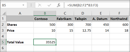
The formula first multiplies the shares (cells B2 – F2) by their prices (cells B3 – F3), and then adds those results to create a grand total of 35,525. This is an example of a single-cell array formula because the formula lives in just one cell.

Press Enter (if you have a current Microsoft 365 Subscription); otherwise press Ctrl+Shift+Enter.

When you press Ctrl+Shift+Enter, Excel automatically inserts the formula between (a pair of opening and closing braces).

To calculate multiple results by using an array formula, enter the array into a range of cells that has the exact same number of rows and columns that you’ll use in the array arguments.

Select the range of cells in which you want to enter the array formula.

Enter the formula that you want to use.

Array formulas use standard formula syntax. They all begin with an equal sign (=), and you can use any of the built-in Excel functions in your array formulas.

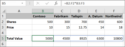
In the following example, the formula multiples shares by price in each column, and the formula lives in the selected cells in row 5.

Press Enter (if you have a current Microsoft 365 Subscription); otherwise press Ctrl+Shift+Enter.

When you press Ctrl+Shift+Enter, Excel automatically inserts the formula between (a pair of opening and closing braces).

If you need to include new data in your array formula, see Expand an array formula. You can also try:

Delete an array formula (you press Ctrl+Shift+Enter there, too)

Name an array constant (they can make constants easier to use)

Источник

Return array in Spreadsheet Function

The code below returns an array. I would like to use it in a spread sheet as an excel formula to return the array. However, when I do, it only returns the first value to the cell. Is there anyway to return the array in a range of equal size as the array?

4 Answers 4

A UDF can certainly return an array, and your function works fine. Just select, e.g., range B2:D2, put =LoadNumbers(1, 3) into the formula bar, and hit Ctrl+Shift+Enter to tell Excel it’s an array function.

Now, you can’t have the UDF auto-resize the range it was called from according to its inputs (at least not without some ugly Application.OnTime hack), but you don’t need to do that anyways. Just put the function in a 1000-cell-wide range to begin with, and have the UDF fill in the unused space with blank cells, like this:

A worksheet formula can only output a value to the same cell the formula was written in. As it stands, the code already produces an array. If you want the values to be shown as you copy the formula down, use a formula like this (in any cell you want) and then copy down:

If you copy down too far, you’ll get a #REF! error because the LoadNumbers ran out of numbers.

I was looking for something similar (create a function in a macro, take inputs from a sheet, output an multi-dim array), and I hope my use-case below helps to answer. If not, my apologies:

Use-case: Create and apply well-known numerical option valuation function, and output the stock price, valuation, and payoff as a 3-D array (3 columns) of #rows as specified in the function (20 in this case, as NAS variable). The code is copied — but the idea is to get the output into the sheet.

a) These inputs are static in the sheet. b) I called the macro formula ‘optval’ via the ‘fx’ function list from an output cell I wanted to start in, and put the starting inputs into the formula. b) The output will propagate to the cells as per the code using the NAS bound of 20 rows. Trivial, but it works. c) you can automate the execution of this and output to the sheet — but anyhow, I hope this way helps anyway.

Источник

Can Excel’s INDEX function return array?

If the data in the range A1:A4 is as follows:

Then INDEX can be used to individually return any value from that list, e.g.

Would return Orange .

Is there a similar Excel functions or combination of functions that would effectively allow you to do something like this:

Which would return an array ?

Is this possible (preferably without VBA), and if so, how? I’m having a tough time figuring out how to accomplish this, even with the use of helper cells.

I can figure out a somewhat complicated solution if the data is numbers (using MMULT ), but the fact that the data is text is tripping me up because MMULT does not work with text.

4 Answers 4

OFFSET is probably the function you want.

But to answer your question, INDEX can indeed be used to return an array. Or rather, two INDEX functions with a colon between them:

This is because INDEX actually returns a cell reference OR a number, and Excel determines which of these you want depending on the context in which you are asking. If you put a colon in the middle of two INDEX functions, Excel says «Hey a colon. normally there is a cell reference on each side of one of these» and so interprets the INDEX as just that. You can read more on this at http://www.excelhero.com/blog/2011/03/the-imposing-index.html

I actually prefer INDEX to OFFSET because OFFSET is volatile, meaning it constantly recalculates at the drop of a hat, and then forces any formulas downstream of it to do the same. For more on this, read my post https://chandoo.org/wp/2014/03/03/handle-volatile-functions-like-they-are-dynamite/

You can actually use just one INDEX and return an array, but it’s complicated, and requires something called dereferencing. Here’s some content from a book I’m writing on this:

The worksheet in this screenshot has a named range called Data assigned to the range A2:E2 across the top. That range contains the numbers 10, 20, 30, 40, and 50. And it also has a named range called Elements assigned to the range A5:B5. That Elements range tells the formula in A8:B8 which of those five numbers from the Data range to display.

If you look at the formula in A8:B8, you’ll see that it’s an array-entered INDEX function: <=INDEX(Data,Elements)>. This formula says, “Go to the data range and fetch elements from it based on whatever elements the user has chosen in the Elements range.” In this particular case, the user has requested the fifth and second items from it. And sure enough, that’s just what INDEX fetches into cells A8:B8: the corresponding values of 50 and 20.

But look at what happens if you take that perfectly good INDEX function and try to put a SUM around it, as shown in A11. You get an incorrect result: 50+20 does not equal 50. What happened to 20, Excel?

For some reason, while =INDEX(Data,Elements) will quite happily fetch disparate elements from somewhere and then return those numbers separately to a range, it is rather reluctant to comply if you ask it to instead give those numbers to another function. It’s so reluctant, in fact, that it passes only the first element to the function.

Consequently, you’re seemingly forced to return the results of the =INDEX(Data,Elements) function to the grid first if you want to do something else with it. Tedious. But pretty much every Excel pro would simply tell you that there’s no workaround. that’s just the way it is, and you have no other choice.

Buuuuuuuut, they’re wrong. At the post http://excelxor.com/2014/09/05/index-returning-an-array-of-values/, mysterious formula superhero XOR outlines two fairly simple ways to “de-reference” INDEX so that you can then use its results directly in other formulas; one of those methods is shown in A18 above. It turns out that if you amend the INDEX function slightly by adding an extra bit to encase that Elements argument, INDEX plays ball. And all you need to do is encase that Elements argument as I’ve done below:

With this in mind, your original misbehaving formula:

. becomes this complex but well-mannered darling:

Источник

Return An Array Using in Excel Using INDEX Function

For any reason, if you want to do some operation on a range with particular indexes, you will think of using INDEX function for getting array of values on specific indexes. Like this.

Let’s Understand it With an Example.

Here, I have a Rate column. I want to sum values at position 1,3, and 5. I write this formula in C2.

Surprisingly, INDEX function does not returns an array of values when we supply an array as indexes. We only get the first value. And SUM function returns the sum of one value only.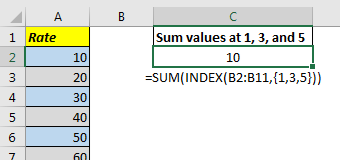

So how do we get INDEX function return that array. Well I found this solution on internet and I don’t really understand how it works, but it works.

The Generic Formula to get Array of Indexes

Range: It is the range in which you want to look for at given index numbers
Number: these are the index numbers.
Now let’s apply above formula to our example.

Write this formula in C2.

And this returns the correct answer as 90.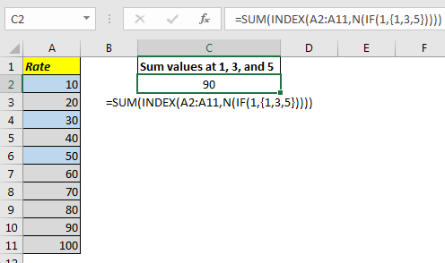

How It Works.

Well, as I said that I don’t know why it works and returns the array of numbers but here what happens.

IF(1,<1,3,5>): This part returns the array <1,3, 5>as expected

N(IF(1,<1,3,5>)) this translates to N(<1,3,5>) which again gives us

NOTE: The N function returns the number equivalent of any value. If a value is not number convertable it returns 0 (like text). And for errors it returns error.

INDEX((A2:A11,N(IF(1,<1,3,5>))): this part translates to INDEX((A2:A11,<1,3,5>) and somehow this returns the array <10,30,50>. As you have seen earlier when write INDEX((A2:A11,<1,3,5>) directly in the formula it only returns 10. But when we use N and IF function it returns the whole array. If you understand it let me know in the comments section below.

How to use cell references for index values to get an array
In the above example, we hardcoded the indexes in function. But what if I want to have it from a range that may change. We replace <1,3,5>with range? Let’s try it.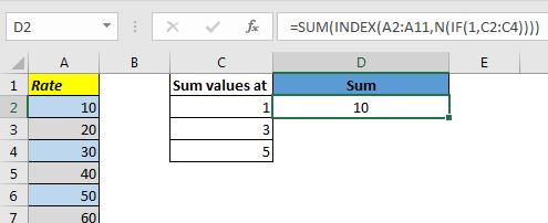

Here we have this formula in Cell D2:

This returns 10. The very first value of the given index. Even if we enter it as an array formula using CTRL+SHIFT+ENTER, it gives the same result.

To make it work add + or — (double unary) operator before range and enter it as array formula.

This works. Don’t ask me how? It just works. If you can tell me how I will include your name and explanation here.
So we learned how to get an array from INDEX function. There’s some crazy stuff going on here in excel. If you can explain how it works here in the comments section below, I will include it in my explanation with your name.

Источник

As the title suggests, we will learn how to create a user-defined function in Excel that returns an array. We have already learned how to create a user-defined function in VBA. So without wasting any time let’s get started with the tutorial.

What is an Array Function?

Array functions are the functions that return an array when used. These function are used with CTRL+SHIFT+ENTER key combinations and this is why we prefer calling array function or formulas as CSE function and formulas.

The excel array function is often multicell array formulas. One example is the TRANSPOSE function.

Creating a UDF array function in VBA

So, the scenario is that I just want to return the first 3 even numbers using function ThreeEven() function.

The code will look like this.

Function ThreeEven() As Integer()

'define array
Dim numbers(2) As Integer

'Assign values to array
numbers(0) = 0
numbers(1) = 2
numbers(2) = 4

'return values
ThreeEven = numbers

End Function

Let us use this function on the worksheet.

You can see that, we first select three cells (horizontally, for vertical we have to use two-dimensional array. We have it covered below.). Then we start writing our formula. Then we hit CTRL+SHIFT+ENTER. This fills the selected cells with the array values.

Note:

In practice, you will not know how many cells you gonna need. In that case always select more cells than expected array length. The function will fill the cells with array and extra cells will show #N/A error.
By default, this array function returns values in a horizontal array. If you try to select vertical cells, all cells will show the first value of array only.

How it works?

To create an array function you have to follow this syntax.

Function functionName(variables) As returnType()

dim resultArray(length) as dataType

'Assign values to array here

functionName =resultArray

End Function

The function declaration must be as defined above. This declared that it is an array function.
While using it on the worksheet, you have to use CTRL+SHIFT+ENTER key combination. Otherwise, it will return the first value of the array only.

VBA Array Function to Return Vertical Array

To make your UDF array function work vertically, you don’t need to do much. Just declare the arrays as a two-dimensional array. Then in first dimension add the values and leave the other dimension blank. This is how you do it:

Function ThreeEven() As Integer()

'define array
Dim numbers(2,0) As Integer

'Assign values to array
numbers(0,0) = 0
numbers(1,0) = 2
numbers(2,0) = 4

'return values
ThreeEven = numbers

End Function

This is how you use it on the worksheet.

UDF Array Function with Arguments in Excel

In the above examples, we simply printed sum static values on the sheet. Let’s say we want our function to accept a range argument, perform some operations on them and return the resultant array.

Example Add «-done» to every value in the range

Now, I know this can be done easily but just to show you how you can use user-defined VBA array functions to solve problems.

So, here I want an array function that takes a range as an argument and adds «-done» to every value in range. This can be done easily using the concatenation function but we will use an array function here.

Function CONCATDone(rng As Range) As Variant()
Dim resulArr() As Variant

'Create a collection
Dim col As New Collection

'Adding values to collection
On Error Resume Next
For Each v In rng
col.Add v
Next
On Error GoTo 0

'completing operation on each value and adding them to Array
ReDim resulArr(col.Count - 1, 0)
For i = 0 To col.Count - 1
resulArr(i, 0) = col(i + 1) & "-done"
Next

CONCATDone = resulArr

End Function

Explanation:

The above function will accept a range as an argument and it will add «-done» to each value in range.

You can see that we have used a VBA collection here to hold the values of the array and then we have done our operation on each value and added them back on a two-dimensional array.

So yeah guys, this is how you can create a custom VBA array function that can return an array. I hope it was explanatory enough. If you have any queries regarding this article, put it in the comments section below.

Click the link below to download the working file:

Related Articles:

Arrays in Excel Formul|Learn what arrays are in excel.

How to Create User Defined Function through VBA | Learn how to create user-defined functions in Excel

Using a User Defined Function (UDF) from another workbook using VBA in Microsoft Excel | Use the user-defined function in another workbook of Excel

Return error values from user-defined functions using VBA in Microsoft Excel | Learn how you can return error values from a user-defined function

Popular Articles:

50 Excel Shortcuts to Increase Your Productivity

The VLOOKUP Function in Excel

COUNTIF in Excel 2016

How to Use SUMIF Function in Excel

Источник

The MAKEARRAY function returns a array with specified rows and columns, based on a custom LAMBDA calculation. MAKEARRAY can be used to create arrays with variable dimensions where the values in the array are calculated.

The MAKEARRAY function takes three arguments: rows, columns, and lambda. Rows is the number of columns to create, and columns is the number or columns to create. Lambda is the calculation to use when creating values in the array. The total number of values in the array returned by MAKEARRAY will equal rows * columns.

LAMBDA structure

The MAKEARRAY uses the LAMBDA function to apply the formula required to calculate array values. The structure of the LAMBDA used by MAKEARRAY is:

LAMBDA(r,c,calculation)

where r represents the row count, and c represents the column count originally passed into MAKEARRAY, and calculation is the formula needed to create the values in the final array.

Note: to generate an array with sequential values, see the SEQUENCE function.

Examples

In the formula below, MAKEARRAY is used to create an array with 2 rows and 3 columns, populated with the result multiplying rows by columns:

=MAKEARRAY(2,3,LAMBDA(r,c,r*c)) // returns {1,2,3;2,4,6}

The result is a 2 x 3 array with six values {1,2,3;2,4,6}.

The calculation can be hardcoded. Below are examples of the same formula, with calculation hardcoded as zero and «x»:

=MAKEARRAY(2,3,LAMBDA(r,c,0)) // returns {0,0,0;0,0,0}
=MAKEARRAY(2,3,LAMBDA(r,c,"x")) // returns {"x","x","x";"x","x","x"}

Random values

MAKEARRAY can be used to generate random values. In the formula below. The CHAR function is used with the RANDBETWEEN function to generate random uppercase letters A-Z:

=MAKEARRAY(2,3,LAMBDA(r,c,CHAR(RANDBETWEEN(65,90))))

The result is a 2 x 3 array like: {«D»,»Q»,»F»;»V»,»C»,»T»}.

Источник