
Excel for Microsoft 365 Excel for Microsoft 365 for Mac Excel for the web Excel 2021 Excel 2021 for Mac Excel 2019 Excel 2019 for Mac Excel 2016 Excel 2016 for Mac Excel 2013 Excel 2010 Excel 2007 Excel for Mac 2011 Excel Starter 2010 More…Less
This article describes the formula syntax and usage of the SIGN function in Microsoft Excel.
Description
Determines the sign of a number. Returns 1 if the number is positive, zero (0) if the number is 0, and -1 if the number is negative.
Syntax
SIGN(number)
The SIGN function syntax has the following arguments:
-
Number Required. Any real number.
Example
Copy the example data in the following table, and paste it in cell A1 of a new Excel worksheet. For formulas to show results, select them, press F2, and then press Enter. If you need to, you can adjust the column widths to see all the data.
|
Formula |
Description |
Result |
|---|---|---|
|
=SIGN(10) |
Sign of a positive number. |
1 |
|
=SIGN(4-4) |
Sign of the result of 4 minus 4 (zero). |
0 |
|
=SIGN(-0.00001) |
Sign of a negative number. |
-1 |
Need more help?
Want more options?
Explore subscription benefits, browse training courses, learn how to secure your device, and more.
Communities help you ask and answer questions, give feedback, and hear from experts with rich knowledge.
In Excel, it is often necessary to use when calculating values that are tied to symbols, the sign of a number, and the type.
The following functions are used for this:
- CHAR;
- TYPE;
- SIGN.
CHAR function makes it possible to get a character with its given code. The function is used to convert the numeric character codes that are received from other computers into characters of the given computer.
TYPE function determines the data types of the cell, returning the corresponding number.
SIGN function returns the sign of a number and returns the value 1 if it is positive, 0 if it is 0, and -1 if it is negative.
Examples of using the CHAR, TYPE and SIGN functions in excel formulas
Example 1. Given a table with character codes: from 65 — to 74:
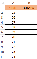
It is necessary with the help of the CHAR to display the characters that correspond to these codes.
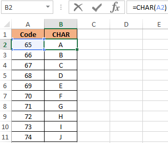
To do this, we enter into the cell B2 the following formula:
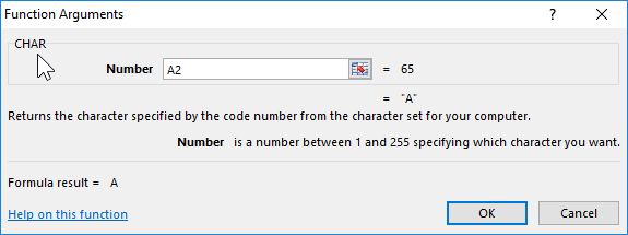
The function argument: Number is the character code.
As a result of the calculations we get:
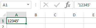
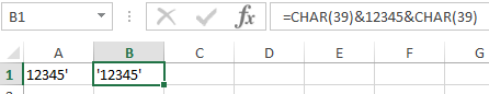
How to use the CHAR in formulas in practice? For example, we need to display a text string in single quotes. For Excel, a single quote as the first character is a special character that converts any cell value to a text data type. Therefore, in the cell itself, the single quote as the first character is not displayed:
To solve this problem, we use the following formula with the function =CHAR(39)
It is also useful to use this function when you need to make a line break in an Excel cell as a formula. And for other similar tasks.
The value 39 in the function argument, you guessed it, is the character code of a single quote.
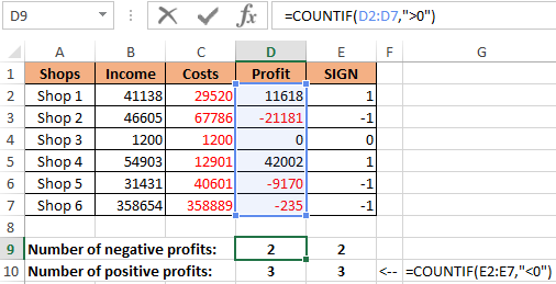
How to count the number of positive and negative numbers in Excel
Example 2. The table contains 3 numbers. Calculate which character has each number: positive (+), negative (-) or 0.
Let’s enter the data in the table of the form:
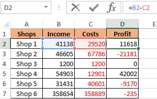
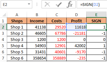
We introduce the formula in cell E2:
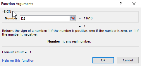
Argument: Number — any real numeric value.
By copying this formula down, we get:
First, we calculate the number of negative and positive numbers in the columns «Profit» and «SIGN»:
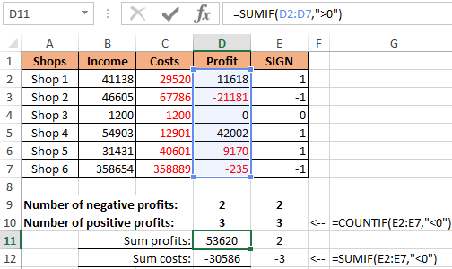
And now we summarize only positive or only negative numbers:
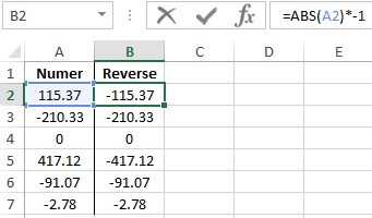
How to make a negative number positive and positive negative? It is very simple to multiply by -1:
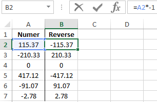
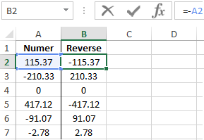
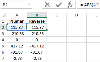
You can even simplify the formula, simply put a subtraction operator sign — minus, before the cell reference:
But what if you need to make a number with any sign positive? Then you should use the ABS function. This function returns any number by module:
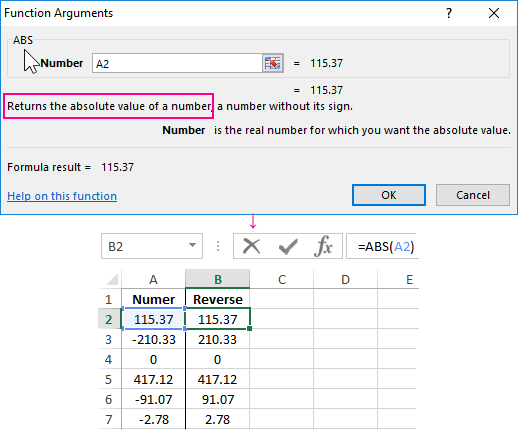
Now it is not difficult to guess how to make any number with a negative minus sign:
Or so:
Checking what types of cell input data in an Excel spreadsheet
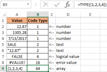
Example 3. Using the TYPE function, display the type of data that is entered in the table:
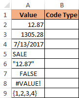
TYPE function returns the code of the data types that can be entered into an Excel cell:
| Data Value | Type Code |
| number | 1 |
| text | 2 |
| logical value | 4 |
| error value | 16 |
| array | 64 |
We introduce the formula for the calculation in cell B2:
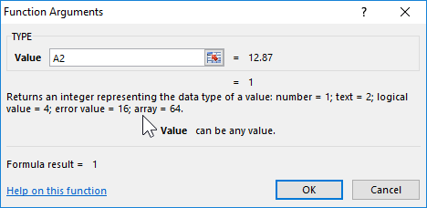
Argument: Value is any valid value.
As a result, we get:
Download examples functions CHAR SIGN TYPE in Excel
Thus, using the TYPE function, you can always check what the Excel cell actually contains. Note that the date is defined by the function as a number. For Excel, any date is a numeric value that corresponds to the number of days that have passed from January 01/01/1900, to the original date. Therefore, each date in Excel should be taken as a numeric data type displayed in the cell format — “Date”.
![]()
Symbols Used in Excel Formula

Here are the important symbols used in Excel Formulas. Each of these special characters have used for different purpose in Excel. Let us see complete list of symbols used in Excel Formulas, its meaning and uses.
Symbols used in Excel Formula
Following symbols are used in Excel Formula. They will perform different actions in Excel Formulas and Functions.
| Symbol | Name | Description |
|---|---|---|
| = | Equal to | Every Excel Formula begins with Equal to symbol (=).
Example:=A1+A5 |
| () | Parentheses | All Arguments of the Excel Functions specified between the Parentheses.
Example:=COUNTIF(A1:A5,5) |
| () | Parentheses | Expressions specified in the Parentheses will be evaluated first. Parentheses changes the order of the evaluation in Excel Formula.
Example: =25+(35*2)+5 |
| * | Asterisk | Wild card operator to to denote all values in a List.
Example: =COUNTIF(A1:A5,”*“) |
| , | Comma | List of the Arguments of a Function Separated by Comma in Excel Formula.
Example: =COUNTIF(A1:A5,“>” &B1) |
| & | Ampersand | Concatenate Operator to connect two strings into one in Excel Formula.
Example: =”Total: “&SUM(B2:B25) |
| $ | Dollar | Makes Cell Reference as Absolute in Excel Formula.
Example:=SUM($B$2:$B$25) |
| ! | Exclamation | Sheet Names and Table Names Followed by ! Symbol in Excel Formula.
Example: =SUM(Sheet2!B2:B25) |
| [] | Square Brackets | Uses to refer the Field Name of the Table (List Object) in Excel Formula.
Example:=SUM(Table1[Column1]) |
| {} | Curly Brackets | Denote the Array formula in Excel.
Example: {=MAX(A1:A5-G1:G5)} |
| : | Colon | Creates references to all cells between two references.
Example: =SUM(B2:B25) |
| , | Comma | Union Operator will combine the multiple references into One.
Example: =SUM(A2:A25, B2:B25) |
| (space) | Space | Intersection Operator will create common reference of two references.
Example: =SUM(A2:A10 A5:A25) |
Share This Story, Choose Your Platform!
6 Comments
-
Redjen
May 31, 2022 at 12:37 pm — Replywhat is the symbol of average in excel?
-
PNRao
June 20, 2022 at 12:40 pm — ReplyYou can use AVERAGE()Function to calculate Average in Excel. If you wants to show the Average Statistical Symbol (x-bar), You can insert from symbols. F7C2 is the Unicode Hexa character for X-bar symbol. Make sure that you have set the Symbol Font :MS Reference Sans Serif.
-
-
Tom Pearce
September 22, 2022 at 3:54 pm — ReplyI have a workbook, where the original author used an @ sign in front of a function call in a formula. I can find no reference as to what the @ does, or how it is used. Any one know??
VBA Example: ActiveSheet.Range(“L2”).Formula = “=@CATEGORY($E2,LFC_AreaLU)”
Note: Category is a User Defined Function in the workbook.-
PNRao
December 5, 2022 at 11:30 am — Reply
-
-
Jane Girard
February 9, 2023 at 8:53 pm — ReplyI have this formula, do you know what the al means in the formula ?
IF(E4=””,””,VLOOKUP(C4,al,5,0)*E4), can-
PNRao
February 27, 2023 at 3:10 am — ReplyIt could be a defined Name or a name of the Table (List Object)
-
© Copyright 2012 – 2020 | Excelx.com | All Rights Reserved
Page load link
This tutorial explains what different symbols mean in formulas in Excel and Google Sheets.
Excel is essentially used for keeping track of data and using calculations to manipulate this data. All calculations in Excel are done by means of formulas, and all formulas are made up of different symbols or operators, depending on what function the formula is performing.
Equal Sign (=)
The most commonly used symbol in Excel is the equal (=) sign. Every single formula or function used has to start with equals to let Excel know that a formula is being used. If you wish to reference a cell in a formula, it has to have an equal sign before the cell address. Otherwise, Excel just shows the cell address as standard text.
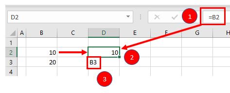
In the above example, if you type (1) =B2 in cell D2, it returns a value of (2) 10. However, typing only (3) B3 into cell D3 just shows “B3” in the cell, and there is no reference to the value 20.
Standard Operators
The next most common symbols in Excel are the standard operators as used on a calculator: plus (+), minus (–), multiply (*) and divide (/). Note that the multiplication sign is not the standard multiplication sign (x) but is depicted by an asterisk (*) while the division sign is not the standard division sign (÷) but is depicted by the forward slash (/).
An example of a formula using addition and multiplication is shown below:
=B1+B2*B3Order of Operations and Adding Parentheses
In the formula shown above, B2*B3 is calculated first, as in standard mathematics. The order of operations is always multiplication before addition. However, you can adjust the order of operations by adding parentheses (round brackets) to the formula; any calculations between these parentheses would then be done first before the multiplication. Parentheses, therefore, are another example of symbols used in Excel.
=(B1+B2)*B3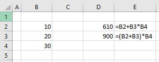
In the example shown above, the first formula returns a value of 610 while the second formula (using parentheses) returns 900.
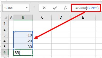
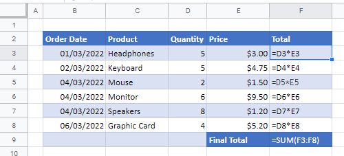
Parentheses are also used with all Excel functions. For example, to sum B3, B4, and B5 together, you can use the SUM Function where the range B3:B5 is contained within parentheses.
=SUM(B3:B5)Colon (:) to Specify a Range of Cells
In the formula used above, the parentheses contain the cell range which the SUM Function needs to add together. This cell range is expressed with a colon (:) where the first cell reference (B3) is the cell address of the first cell included in the range of cells to add together, while the second cell reference (B5) is the cell address of the last cell included in the range.
Dollar Symbol ($) in an Absolute Reference
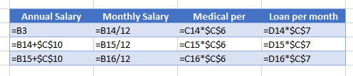
A particular useful and common symbol used in Excel is the dollar sign within a formula. Note that this does not indicate currency; rather, it’s used to “fix” a cell address in place in order that a single cell can be used repetitively in multiple formulas by copying formulas between cells.
=C6*$C$3By adding a dollar sign ($) in front of the column header (C) and the row header (3), when copying the formula down to Rows 7–15 in the example below, the first part of the formula (e.g., C6) changes according to the row it is copied down to while the second part of the formula ($C$3) stays static always enabling the formula to refer to the value stored in cell C3.
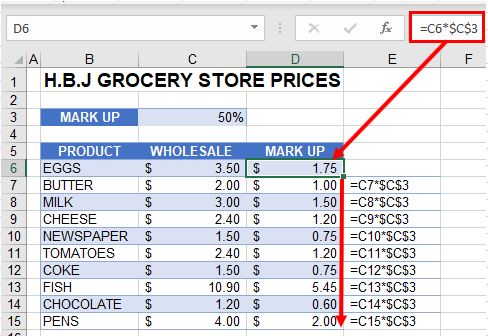
See: Cell References and Absolute Cell Reference Shortcut for more information on absolute references.
Exclamation Point (!) to Indicate a Sheet Name
The exclamation point (!) is critical if you want to create a formula in a sheet and include a reference to a different sheet.
=SUM(Sheet1!B2:B4)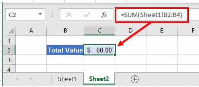
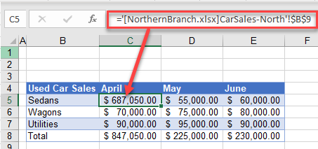
Square Brackets [ ] to Refer to External Workbooks
Excel uses square brackets to show references to linked workbooks. The name of the external workbook is enclosed in square brackets, while the sheet name in that workbook appears after the brackets with an exclamation point at the end.
Comma (,)
The comma has two uses in Excel.
Refer to Multiple Ranges
If you wish to use multiple ranges in a function (e.g., the SUM Function), you can use a comma to separate the ranges.
=SUM(B2:B3, B6:B10)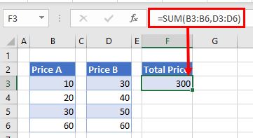
Separate Arguments in a Function
Alternatively, some built in Excel functions have multiple arguments which are usually separated with commas. (These can also be semicolons, depending on the function syntax.)
=VLOOKUP(H5, B6:E15, 4, FALSE)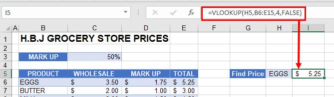
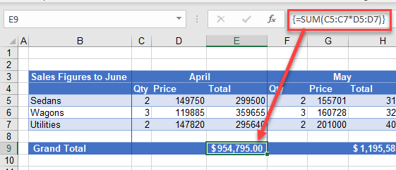
Curly Brackets { } in Array Formulas
Curly brackets are used in array formulas. An array formula is created by pressing the CTRL + SHIFT + ENTER keys together when entering a formula.
Other Important Symbols
| Symbol | Description | Example |
|---|---|---|
| % | Percentage | =B2% |
| ^ | Exponential operator | =B2^B3 |
| & | Concatenation | =B2&B3 |
| > | Greater than | =B2>B3 |
| < | Less than | =B2<B3 |
| >= | Greater than or equal to | =B2>=B3 |
| <= | Less than or equal to | =B2<=B3 |
| <> | Not equal to | =B2<>B3 |
Symbols in Formulas in Google Sheets
The symbols used in Google Sheets are identical to those used in Excel.
The SIGN function in Excel is a Maths/Trig function that gives us this result. The SIGN function returns the sign (-1, 0, or +1) of the supplied numerical argument. The SIGN formula in Excel can be used by typing the keyword: =SIGN( and providing the number as input.
For example, suppose we have a dataset of sales of a product for two years in cells A1(80,000) and B1(50,000). Now, we want to see if there is an increase in the figure compared to last year. In such a scenario, we can use the following SIGN formula:
=SIGN(A1-B1)
=+1.
Table of contents
- SIGN Function in Excel
- Syntax
- How to Use SIGN Function in Excel? (with Examples)
- Example #1
- Example #2
- Example #3
- Example #4
- Example #5
- SIGN Excel Function Video
- Recommended Articles
Syntax

Arguments
the number: It is the number to get the sign for.
The input number can be any number entered directly or in the form of any mathematical operation or cell referenceCell reference in excel is referring the other cells to a cell to use its values or properties. For instance, if we have data in cell A2 and want to use that in cell A1, use =A2 in cell A1, and this will copy the A2 value in A1.read more.
Output:
The SIGN formula in Excel has only three results: +1, 0, and -1.
- If the number exceeds zero, the Excel SIGN formula will return 1.
- If the number equals zero, the SIGN formula in Excel will return 0.
- If the number is less than zero, the SIGN formula in Excel will return -1.
If the supplied number argument is non-numeric, the Excel SIGN function will return #VALUE! Error.
How to Use the SIGN Function in Excel? (with Examples)
You can download this SIGN Function Excel Template here – SIGN Function Excel Template
Example #1
Suppose you have the final balance figures for seven departments for 2016 and 2017, as shown below.
| Departments | 2016 | 2017 |
|---|---|---|
| Department A | 10000 | 12000 |
| Department B | -1890 | -2000 |
| Department C | 250000 | 320000 |
| Department D | 80000 | 60000 |
| Department E | -50000 | -40000 |
| Department F | -1000 | 2500 |
| Department G | 12000 | 12500 |
Some departments are running in debt, and some are giving good returns. Now, you want to see if there is an increase in the figure compared to last year. To do so, you can use the following SIGN formula for the first one.
=SIGN(D4 – C4)

It will return +1. The argument to the SIGN function is a value returned from other functions.

Drag it to get the value for the rest of the cells.

Example #2
In the above example, you may also want to calculate the percentage increase in excelPercentage increase = (New Value — Old Value)/ Old Value. Instead of showing the delta as a Value, percentage increase shows how much the value has changed in terms of percentage increase.read more concerning the previous year.
For that, you can use the following SIGN formula:
=(D4 – C4)/C4 * SIGN(C4)

Drag it to the rest of the cells.

If the balance for 2016 is zero, the function will give an error. Alternatively, we may use the following SIGN formula to avoid the error:
=IFERROR((D4 – C4) / C4 * SIGN(C4), 0)
To get the overall percentage of increase or decrease, you can use the following formula:
(SUM(D4:D10) – SUM(C4:C10)) / SUM(C4:C10) * SIGN(SUM(C4:C10))

SUM(D4:D10) will give the net balance including all departments for 2017
SUM(C4:C10) will give the net balance including all departments for 2016
SUM(D4:D10) – SUM(C4:C10) will give the net gain or loss, including all departments.
(SUM(D4:D10) – SUM(C4:C10)) / SUM(C4:C10) * SIGN(SUM(C4:C10)) will give the percentage gain or loss
Example #3
Suppose you have a list of numbers in B3:B8, as shown below.

Now, you want to change the negative number’s sign to positive.
You may use the following formula:
=B3 * SIGN(B3)

If the B3 is negative, SIGN(B3) is -1, and B3 * SIGN(B3) will be negative * negative, which will return positive.
If the B3 is positive, SIGN(B3) is +1, and B3 * SIGN(B3) will be positive * positive, which will return positive.
It will return to 280.

Drag it to get the values for the rest of the numbers.

Example #4
Suppose you have your monthly sales in F4:F10 and want to find out if your sales are going up and down.
To do so, you can use the following formula:
=VLOOKUP(SIGN(F5 – F4), A5:B7, 2)
A5:B7 contains the information on the up, zero, and down.
The SIGN function will compare the current and previous month’s sales using the SIGN function. The VLOOKUPThe VLOOKUP excel function searches for a particular value and returns a corresponding match based on a unique identifier. A unique identifier is uniquely associated with all the records of the database. For instance, employee ID, student roll number, customer contact number, seller email address, etc., are unique identifiers.
read more Excel function will pull the information from the VLOOKUP table and return whether the sales are going up, zero, or down.

Drag it to the rest of the cells.

Example #5
Suppose you have sales data from four zones: East, West, North, and South for products A and B, as shown below.
| Zone | Product | Quantity | Price | Sales |
|---|---|---|---|---|
| East | A | 2 | 1000 | 2000 |
| East | B | 1 | 1500 | 1500 |
| West | A | 4 | 1200 | 4800 |
| North | A | 3 | 1500 | 4500 |
| North | B | 5 | 1000 | 5000 |
| West | B | 10 | 1300 | 13000 |
| South | A | 6 | 1200 | 7200 |
| South | B | 12 | 1500 | 18000 |
| East | A | 3 | 1100 | 3300 |
| North | B | 4 | 1200 | 4800 |
| West | B | 5 | 1300 | 6500 |
Now, you want the total sales for product A or East zone.
It can be calculated as:
=SUMPRODUCT(SIGN((B4:B15 = “EAST”) + (C4:C15 = “A”)) * F4:F15)

Let us see the above SIGN function in detail.
B4:B15 = “EAST”
It will give 1 if it is “EAST” else it will return 0. It will return {1, 1, 0, 0, 0, 0, 0, 0, 1, 0, 0}
C4:C15 = “A”
It will give 1 if it is “A” else it will return 0. It will return {1, 0, 1, 1, 0, 0, 1, 0, 1, 0, 0}
(B4:B15 = “EAST”) + (C4:C15 = “A”)
It will return sum the two and {0, 1, 2}. It will return {2, 2, 1, 1, 0, 0, 1, 0, 2, 0, 0}
SIGN((B4:B15 = “EAST”) + (C4:C15 = “A”))
It will then return {0, 1} here since there is no negative number. It will return {1, 1, 1, 1, 0, 0, 1, 0, 1, 0, 0}.
SUMPRODUCT(SIGN((B4:B15 = “EAST”) + (C4:C15 = “A”)) * F4:F15)
It will first take the product of the two matrix {1, 1, 1, 1, 0, 0, 1, 0, 1, 0, 0} and {2000, 1500, 4800, 4500, 5000, 13000, 7200, 18000, 3300, 4800, 6500} which will return {2000, 1500, 4800, 4500, 0, 0, 7200, 0, 3300, 0, 0}, and then sum it.
It will finally return 23,300.

Similarly, to calculate the product sales for East or West zones, you may use the following SIGN formula:
=SUMPRODUCT(SIGN((B4:B15 = “EAST”) + (B4:B15 = “WEST”)) * F4:F15)
For product A in East zone:
=SUMPRODUCT(SIGN((B4:B15 = “EAST”) * (C4:C15 = “A”)) * F4:F15)
SIGN Excel Function Video
Recommended Articles
This article is a guide to SIGN Function in Excel. Here, we discuss the SIGN formula in Excel and how to use the SIGN function, along with Excel examples and downloadable Excel templates. You may also look at these useful functions in Excel: –
- VLOOKUP Multiple CriteriaSometimes while working with data, when we match the data to the reference Vlookup, it finds the first value and does not look for the next value. However, for a second result, to use Vlookup with multiple criteria, we need to use other functions with it.read more
- COUNTIF Multiple CriteriaIn Excel, the COUNTIF with multiple criteria method can be used with the concatenation operator or the & operator in criteria or the or operator as required.read more
- SUMPRODUCT in ExcelThe SUMPRODUCT excel function multiplies the numbers of two or more arrays and sums up the resulting products.read more
- MONTH ExcelThe Month Function is a date function that determines the month for a given date in date format. It takes an argument in a date format and displays the result in integer format.read more