
Excel for Microsoft 365 Excel 2021 Excel 2019 Excel 2016 Excel 2013 Excel 2010 Excel 2007 More…Less
Functions are predefined formulas that perform calculations by using specific values, called arguments, in a particular order, or structure. Functions can be used to perform simple or complex calculations. You can find all of Excel’s functions on the Formulas tab on the Ribbon:

-
Excel function syntax
The following example of the ROUND function rounding off a number in cell A10 illustrates a function’s syntax.

1. Structure. The structure of a function begins with an equal sign (=), followed by the function name, an opening parenthesis, the arguments for the function separated by commas, and a closing parenthesis.
2. Function name. For a list of available functions, click a cell and press SHIFT+F3, which will launch the Insert Function dialog.
3. Arguments. Arguments can be numbers, text, logical values such as TRUE or FALSE, arrays, error values such as #N/A, or cell references. The argument you designate must produce a valid value for that argument. Arguments can also be constants, formulas, or other functions.
4. Argument tooltip. A tooltip with the syntax and arguments appears as you type the function. For example, type =ROUND( and the tooltip appears. Tooltips appear only for built-in functions.
Note: You don’t need to type functions in all caps, like =ROUND, as Excel will automatically capitalize the function name for you once you press enter. If you misspell a function name, like =SUME(A1:A10) instead of =SUM(A1:A10), then Excel will return a #NAME? error.
-
Entering Excel functions
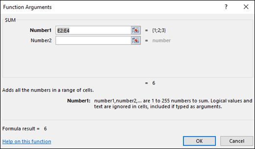
When you create a formula that contains a function, you can use the Insert Function dialog box to help you enter worksheet functions. Once you select a function from the Insert Function dialog Excel will launch a function wizard, which displays the name of the function, each of its arguments, a description of the function and each argument, the current result of the function, and the current result of the entire formula.
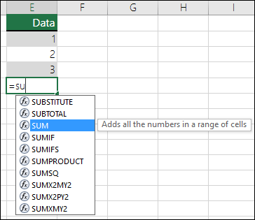
To make it easier to create and edit formulas and minimize typing and syntax errors, use Formula AutoComplete. After you type an = (equal sign) and beginning letters of a function, Excel displays a dynamic drop-down list of valid functions, arguments, and names that match those letters. You can then select one from the drop-down list and Excel will enter it for you.
-
Nesting Excel functions
In certain cases, you may need to use a function as one of the arguments of another function. For example, the following formula uses a nested AVERAGE function and compares the result with the value 50.
1. The AVERAGE and SUM functions are nested within the IF function.
Valid returns When a nested function is used as an argument, the nested function must return the same type of value that the argument uses. For example, if the argument returns a TRUE or FALSE value, the nested function must return a TRUE or FALSE value. If the function doesn’t, Excel displays a #VALUE! error value.
Nesting level limits A formula can contain up to seven levels of nested functions. When one function (we’ll call this Function B) is used as an argument in another function (we’ll call this Function A), Function B acts as a second-level function. For example, the AVERAGE function and the SUM function are both second-level functions if they are used as arguments of the IF function. A function nested within the nested AVERAGE function is then a third-level function, and so on.

Need more help?
In Excel 2013, data functions help you locate specified data from your lists of data. For example, if you have a worksheet that has a list of a thousand of your employees, along with their ages, you can use a data function to find an employee’s location in a worksheet. This is easier than scrolling through countless rows. You can also find the employee and then find their age. In short, data functions give you various ways to search your data.
In this article, we are going to talk about:
-
The MATCH function
-
The INDEX function
-
Handling #REF errors
-
The CHOOSE function
-
Using the MATCH AND INDEX functions together
The MATCH Function
The MATCH lets you check an item against the list, and it will tell you where it appears in the list.
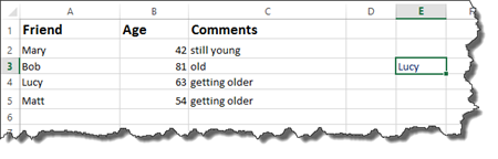
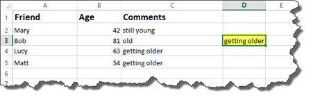
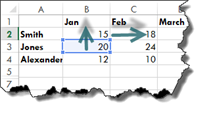
Take a look at our spreadsheet below.
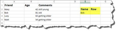
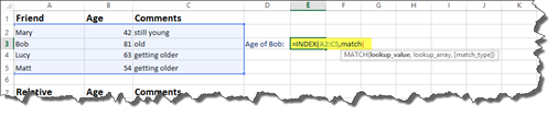
We are going to use the MATCH function to find the row in the list (on the left) where the name Bob is found.
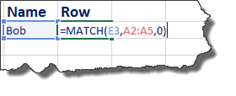
To find this, we are going to type:
The MATCH function asks for the:
-
Lookup_value . In this case, that value is E3. This is where we’ve written Bob’s name as the name we will search for. Instead of E3, we could have also typed «Bob» in our formula.
-
Lookup_array is the range of cells where the data will be found. We selected the column.
-
Match_type is 0 or 1. 0 is an exact match. -1 is less than. 1 is greater than.
Press Enter.
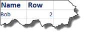
Excel tells us that Bob’s name is in row 2.
Note: If there had been two Bobs in our list, it would only show the location of the first Bob. The MATCH function only returns the first match.
In our example, we searched for text. The text we searched for was «Bob.»
When you search for text, you will search for the exact value (0) for the match_type. You may also use wildcards, as we’ll learn about shortly.
However, if you are searching for numerical data using the MATCH function, -1 would return the first match that was LESS than the value you are searching for. 1 would return the first match that was GREATER than the value you are searching for.
In the example above, if we replaced Bob with the number 10, a match_type of -1 would search for the first value that was less than 10. 1 would search for the first value that was greater than 10.
About the Wildcard Feature
As we mentioned, the MATCH function also has a wildcard feature. The wildcard feature allows you to look for parts of a name.
For example, if we were looking for a name that began with Ma, we could use the MATCH function with the wildcard feature.
The wildcard feature is actually just an asterisk.
Take a look at our formula below:
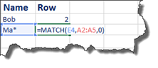
Notice that the asterisk was placed in the cell that we referenced as the lookup_value.
Press Enter.
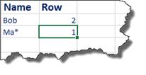
We are shown that a name that begins with Ma is located in row 1. If we look at our list, this name is Mary.
In addition:
-
You can put an asterisk at the beginning of a name. For example, to find names that end with -es.
-
You can put a question mark for a single wild card character, such as Ma?y.
The INDEX Function
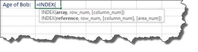
The INDEX function will give you the value of a cell that’s at a specified location.
Below, we are going to use the INDEX function.
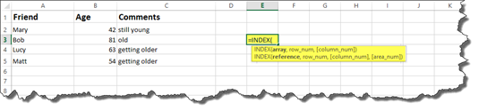
Notice that the INDEX function has two sets of parameters. You can use either one.
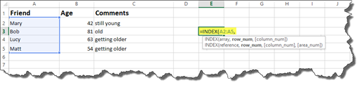
Let’s use the first set of parameters first which is INDEX(array,row_num,[column_num]).
For this example, let’s say our array is a column of cells. We’ve selected those cells below.
Next, we enter a row number.
We are going to enter 3.
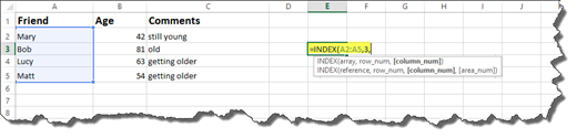
The number three stands for the 3rd position in the array we selected, or the third row in the array we’ve selected.
Close out the formula using an end bracket.
Hit Enter.
If we wanted to use the INDEX function to find a value in an area (both columns and rows), then we could also use the [column_num] parameter. However, this is optional.
Let’s see how it works. Let’s say we want to find a value in a range of cells that contains columns and rows.
You would enter =INDEX( then select the range of cells for your array. In our last example, we only selected a column for our array, now we select rows and columns.
Next, enter the row number, then the column number. Close out the Formula.
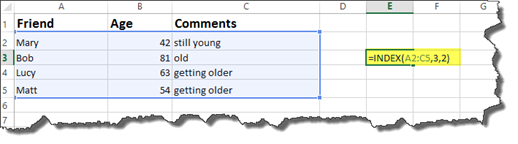
Press Enter.
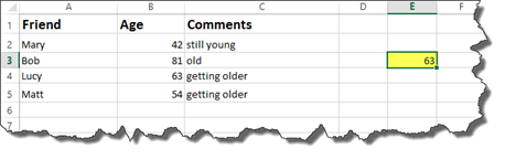
Remember, row 3 is actually position three. Based on our selected array, that is actually row 4 in the spreadsheet.
Column 2 is actually position two. Position two is the age column. If we scroll down to position three, we can see that the value is 63, the same value that we see returned below.

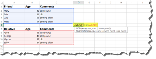
Now, let’s look at the second set of parameters for the INDEX function.
The second set of parameters asks for a reference instead of an array.
A reference is a group of arrays.
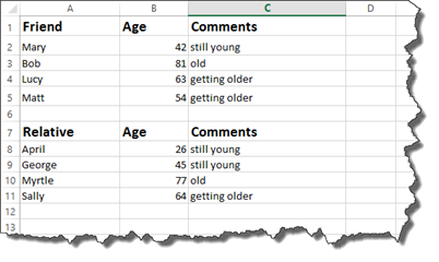
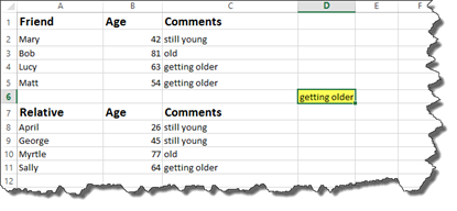
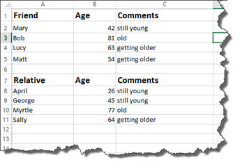
In our worksheet below, we have two different lists. One is for friends. The other is for relatives. We are going to select two sets of arrays. One list will be one array. The other list will be the second array.
Here is how we enter it:
We now have our reference parameter.
Enter a row number.
Enter a column number.
The area_number parameter is optional.
Close the formula.
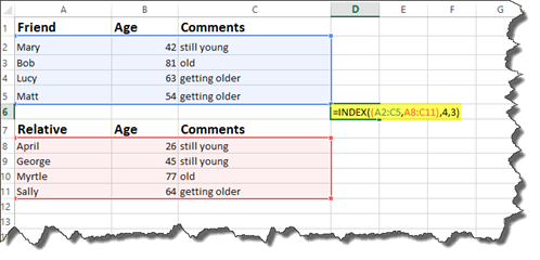
Press Enter.
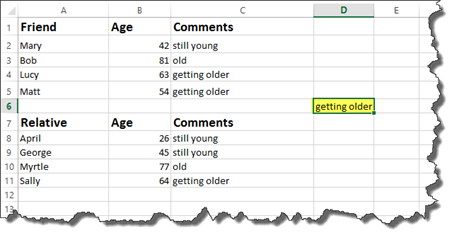
Our results our «getting older.» This is indeed row 4, column 3, but that’s only for the first array – or area that we selected.
If we want Excel to look at the second area we’ve selected, we need to use the optional area_number parameter.
We are going to enter 2 for the area_number. The area_number is determined by the order they appear in the reference section.
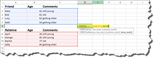
This will return results in the second area, or the area where we have relatives.
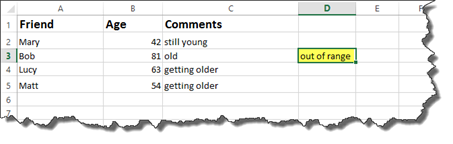
Out of Range Requests
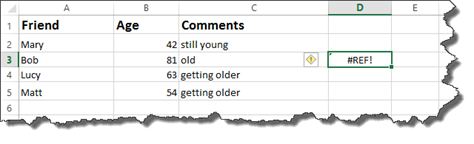
If you use an INDEX function, then enter a row or column number as a parameter, and that row or column doesn’t exist, you will get a #REF error.
Take a look at the snapshot below.
We entered row 6 as the row number.
What we want to do is make that error message look better – and to also better communicate what the problem is.
Let’s put an IF statement into our formula.
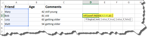
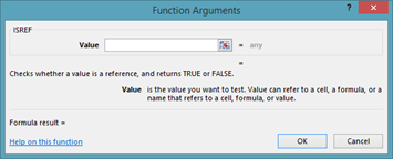
We are going to use the ISREF function to run a logical test. The ISREF function checks to see if certain cells reference one another.
This is how we would enter it:
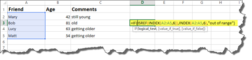
In the snapshot above, you can see what we specify to appear in the cell for the value if true, as well as the value if false.
Press Enter.
We no longer have a #REF message in the cell. Now it simply says out of range.
You can also find the ISREF function by going to Formulas>More Functions>Information>ISREF.
The Functions Arguments dialogue box is shown below:
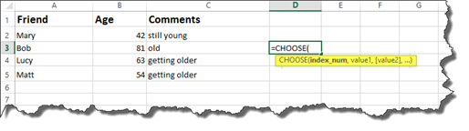
The CHOOSE Lookup Function
The CHOOSE function is another lookup function. Whereas the INDEX function deals with ranges or groups of ranges, the CHOOSE function deals with individual cells.
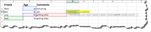
You can see the parameters for the CHOOSE function highlighted below.
Index_num refers to the number of the item in a comma separated list of cells.
In our worksheet, we want to search the 2nd item in our comma separated list.
We would enter the number 2, then select the cells we want to look up, separating each of them with a comma, as shown below.
These are value1, value2, value2, etc., all the way up to value254. This means you can have up to 254 values. You can also have groups of ranges.
Close the brackets when you’re finished entering values.
Hit Enter.
We can see our returned value is «getting older.» This is indeed the second value we selected.
Using the MATCH and INDEX Functions Together
When you use the MATCH and INDEX functions together, you can use them as an alternative to VLOOKUP and HLOOKUP. In fact, they can be quicker and easier to use.
Let’s look at how to use the MATCH and INDEX functions together.
Take a look at our worksheet below.
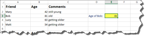
Let’s say we want to determine the age of Bob.
We start out using the INDEX function.
Next, we select the array of cells.
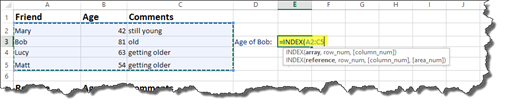
Enter a comma, then the match function.
Now we enter the formula for the MATCH function.
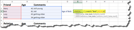
In the snapshot above, the lookup_value is «Bob.» We selected the lookup_array, which is A2:A5. We entered 0 because we want an exact match.
Now let’s enter a comma and return to finish the INDEX function.
We need to specify which column. This is another MATCH function.
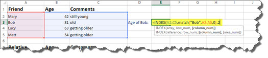
We want to search column 2.
Close the brackets, then press Enter.
NOTE: If you needed to, you could use another MATCH function for the column parameter as well. In other words, you can use more than one MATCH function when using INDEX and MATCH together.
—————-
Continuing with Data Functions
We will discuss:
-
The IS functions, including ISERR and ISERROR
-
The IFFERROR function
-
The OFFSET function
-
How to create a dynamic range using the OFFSET function
-
How to create a dynamic formula using the INDIRECT function
-
How to deal with INDIRECT function errors
-
The CELL Function
The IS Functions
In Excel 2013, the IS functions return logical true or false values. IS functions are used to get information regarding a value before it takes another action, such as solving a formula. In conjunction with IF statements, we told Excel what we wanted to appear on the screen if the outcome was true or if it was false. In short, IS functions check for errors.
The ISERR and ISERROR Functions
As we just said, IS functions check for errors.
Now let’s take a look at how to use them.
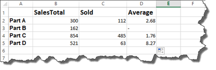
Take a look at our worksheet below.
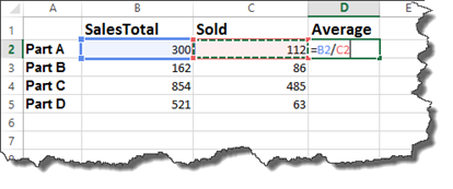
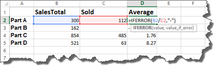
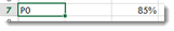
In this example, we have four different parts that were sold. The SalesTotal column shows the dollar amount earned from all sales.
The Sold column shows how many were sold.
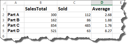
In the Average column, we’ve entered a formula to produce the average price per product sold.
Let’s press Enter, then complete the average for each part.
If we remove a value from the SOLD column, we will get an error message.
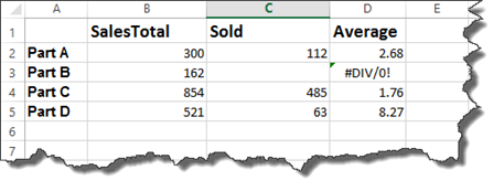
Excel is letting us know we are trying to divide by 0.
To prevent us from seeing those unattractive error messages, we can use the ISERR function to check for errors as we calculate formulas.
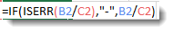
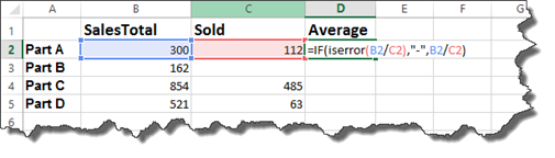
Instead of entering =B2/C2 as we did in cell D2 to calculate the average, we will instead enter the ISERR function along with the formula. If there’s an error, we want a dash to appear. If there’s not an error, we want Excel to calculate the formula and display the results.
Let’s look at how we enter it.
First, we enter =IF(iserr for the ISERR function, then an open bracket.

Enter the formula that you want to calculate.
Ours is C2/D2.
Close the brackets.
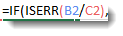
Enter a comma.
What we have said is this: If there is an error when you divide C2/D2…
Next, we have to tell Excel what to do.
If it’s true, and there is an error, we want Excel to display a dash.
If it’s false, and there is not an error, we want Excel to calculate the formula and display the results.
Press Enter, then finish completing the average for each product.
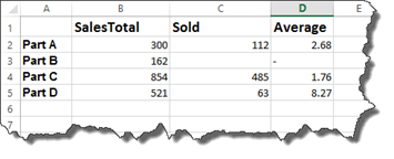
The error message that was showing for Part B is now a dash.
The ISERROR function works in the same way.
Hit Enter.
You can then finish the worksheet by dragging the handle in the lower right corner of the cell.
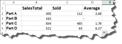
As you can see, when there was an error, Excel returned a dash.
NOTE: You can also find the IS functions under Formulas>More Functions>Information
The IFERROR Function
The IFERROR function is a shortcut, per se, to the ISERR and ISERROR functions.
With the IFERROR function, you simply enter =IFERROR, then the parameters in brackets.
The first parameter is the value that you want to test for an error. If we use the previous worksheet, it’s C2/D2.
Next, is the value_if_error. Enter what you want displayed in the cell if an error is found.
You can see the IFFERROR function below.
Press Enter.
If you look at our worksheet, you’ll see the IFERROR put a dash in the cell where there was an error.
The OFFSET Function
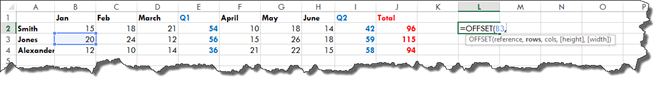
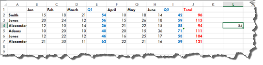
The OFFSET function returns the address of a cell or range of cells by using a reference cell. When you use the OFFSET function, you select a cell or range of cells that are offset from a location.
Let’s take a look at the OFFSET function in an actual worksheet to better understand the purpose it serves.
Here is the worksheet.
Now let’s enter in our formula.
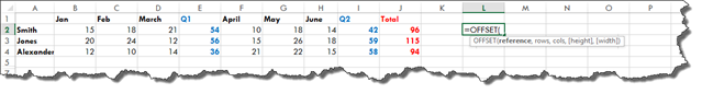
The first parameter asked for when you use an OFFSET function is a reference. This is the starting point. After you enter the reference, Excel wants to know how many rows and columns offset from the starting point that you want to be.
Let’s choose our reference.
Now we have to decide how many rows offset we want to be. This can be a positive or negative number. A positive number takes us down, a negative number takes us up.
Let’s use -1.
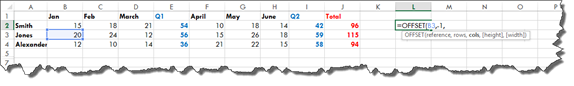
This will move us up one cell on the worksheet.
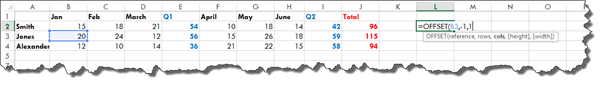
Next, enter the number of columns. A negative number will move to the left. A positive number moves to the right. You can also enter zero to stay in the same column.
The final two parameters that you can enter are optional. They are height and width. We will talk about those in another example.
NOTE: You can also enter formulas for any of the parameters to perform a calculation that determines how far you move from the starting point.
For now, add a closing bracket, then press Enter.
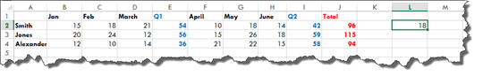
If we count cells from out starting point, we can see that is up one cell and to the right one cell.
In our example, we offset a single cell. If we want to offset an entire range, we will use the height and width parameters we mentioned just a second ago.
Let’s take a look at how to do it.
As you can see, we have expanded our worksheet.
We start off the same as we did with the last example by choosing the reference cell, then the number of rows and columns.
However, now we are going to enter how many rows to include (height) and how many columns to include (width).
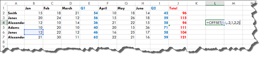
We have extended our range by two rows and two columns.
The offset is now defining a range.
Press Enter.
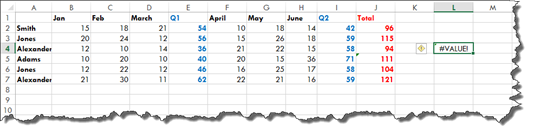
This causes us to get a #VALUE! error because Excel doesn’t know what to do with the range.
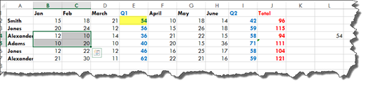
To eliminate the error, the range can be embedded in a sum. It can also be embedded in any other type of function, such as COUNT, MIN, MAX, etc.
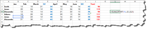
Press Enter.
We now get 54.
54 is the sum of the four cells selected below that define our range:
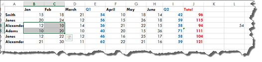
It is the total shown in our highlighted cell below.
Creating a Dynamic Named Range
At first glance, it’s easy to wonder in what situation you would ever use an OFFSET function. A real world example of using the OFFSET function is in creating dynamic named ranges, as we’re going to show you how to do.
Take a look at our invoice below.
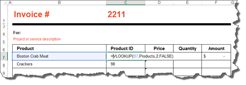
If you also remember, we named our data range in our products worksheet, shown below.
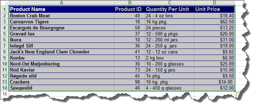
However, when we tried to add a new product at the end of the range, Excel didn’t include it in the named range. As a result, we couldn’t enter it into our invoice. At that time, we decided to insert the new row in the middle of existing rows so that it would be included in the named data range.
Now, we are going to solve that problem. We are going to use the OFFSET function to make it so that our named range dynamically increases in size. This means if we add a new row to the bottom of the named range, the named range will automatically expand.
Our named range is currently titled Products.
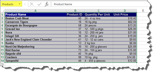
Let’s learn to turn it into a dynamically named range.
Click the Name Manager button under the Formulas tab.
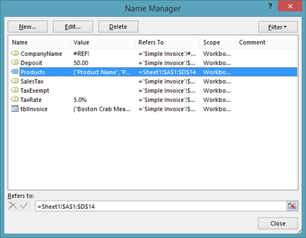
We have clicked on Products.
Go down to the Refers To field at the bottom of the dialogue box.
It’s there that we can start to enter our OFFSET function.
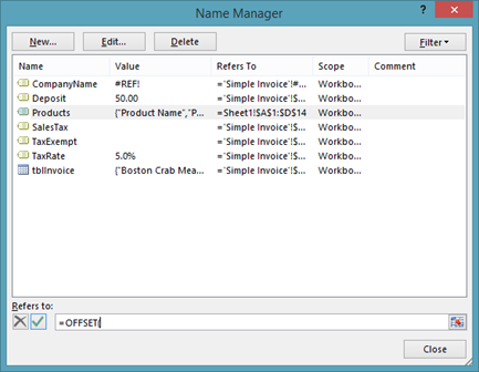
Let’s finish adding it.
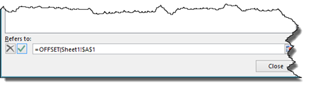
The first thing we entered was our reference. Our reference is our worksheet since this worksheet contains our product list. This is titled Sheet1. We put an exclamation point to let Excel know we are referencing the worksheet. Then, we put the cell that we are referencing, which is the very first cell in the worksheet.
Now we have to tell Excel how many rows we’d like to move. We want to enter 0. We also want to enter zero for the number of columns.
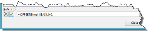
We are not trying to offset the starting point; instead, we are using it to highlight a range.
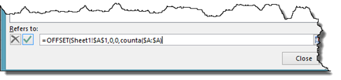
Now we have to enter the height – or how many rows.
Instead of trying to count them on the worksheet, we will use the COUNTA function. The COUNTA function counts the number of cells that have data. We are going to specify that it count the number of cells in column A.
Next, we add in the width – or the number of columns. We can use another COUNTA function, but since, in our example, we are unlikely to add columns, we’re just going to add the number.
Enter a closing bracket.
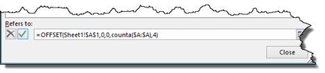
Press the green checkmark button to the left of the formula, then press Close.
Now if we add rows to the product list, it would automatically be included in our dynamic name range.
Creating a Dynamic Formula Using the INDIRECT Function
There might be times when you don’t have the actual cell to reference, but you have a cell with a reference to the actual cell in it. This is where you would use the INDIRECT function.
That may sound confusing.
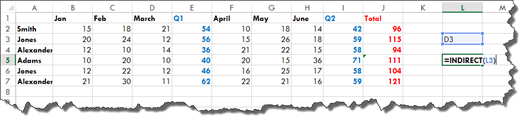
To show you what we mean, take a look at our worksheet below.
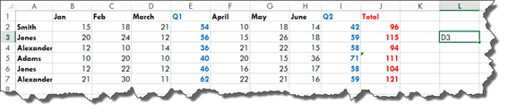
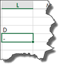
In cell L3, we are referencing cell D3.
We want the value of cell D3 to appear in cell L5.
The easiest thing to do, especially in very large worksheets, would be to use cell L3 to reference cell D3.
Let’s try to do that.
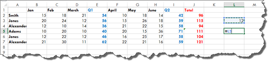
Press Enter.
As you can see, Excel returns D3.
That’s not what we want. We want the value of the referenced cell.
To get that, we will use an INDIRECT function.
The first parameter is the reference, which is cell L3, as shown below.
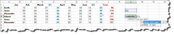
Next, you can decide the optional parameters. As you can see above, we can choose either FALSE or TRUE. FALSE means what we reference will be interpreted as R1C1 – or row 1 column 1. TRUE means it will be interpreted as A1, which is a cell.
We want true since we are referencing a cell.
TRUE is the default choice, so you don’t need to actually enter TRUE. You can just enter a closing bracket if you want.
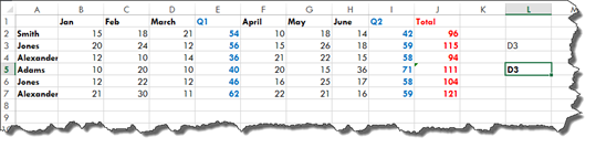
Press Enter.
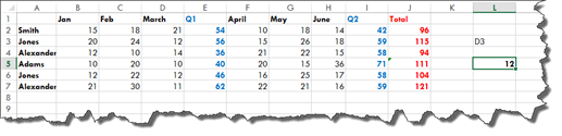
You can now see the value of cell D3 in cell L5.
We are essentially using cell L3 to link to D3. The INDIRECT function picks up whatever cell reference we have in L3 and displays the value of that cell.
We can now change the cell reference in L3, and it will display the value of that cell in L5.
INDIRECT functions can be used inside other functions as well. You can also use them to select and create whole ranges.
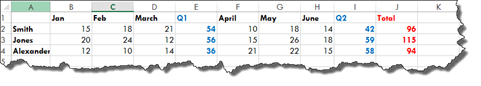
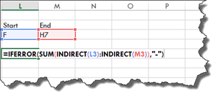
Let’s say we want to add a range of cells. The start cell – or where we want the range to start— is B2. The end cell – or where we want the range to end – is D7. This will effectively add the total sales for Q1.
In our worksheet below, we’ve entered the start and end cells.
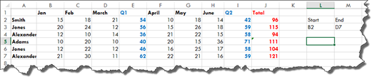
Now let’s enter it into cell L5.
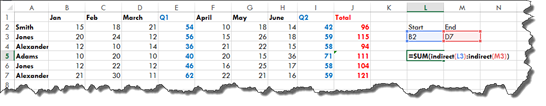
In the example above, we used SUM, but you can use any function that you want.
We have instructed Excel to add the values of the cells referenced in L3 and M3. Right now, L3 and M3 reference B2 and D7 respectively.
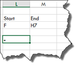
Press Enter.
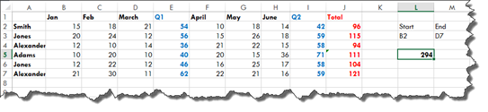
This is the total of our Q1 sales. If you want, you can double check this by adding up the totals in the Q1 column.
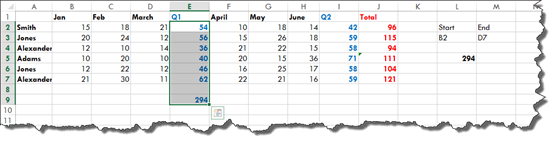
As you can see, it equals 294.
Now, we can go back to L3 and M3 and change the cell references. Let’s say we want the total for Q2.
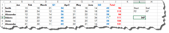
It now gives us the total.
INDIRECT Errors
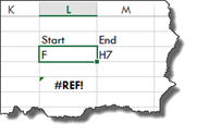
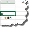
With INDIRECT functions, if you add a cell reference that’s not actually a cell reference, you will see the #REF error.
For example, instead of entering F2 as our starting point, we’ve entered just F below. That’s not an actual cell reference. A cell reference needs a row and column.
We get the #REF error message.
We can use the IFERROR function that we learned about earlier in this section to determine what is displayed if there is a #REF error.
All we need to do is enter =IFFERROR( before our INDIRECT function, as shown below, then specify the message that’s displayed if there is an error.
Press Enter.
Let’s use a simpler example so you can see exactly how the IFERROR function is added.
Let’s use our earlier example when we simply reference cell D3, except we are going to make it so we get an error.
Let’s double click on the #REF error, and add the IFERROR function.
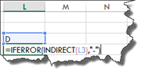
We have essentially told Excel that if there is an error with the INDIRECT function, to display a dash.
Press Enter.
The CELL Function
We have learned to create dynamic formulas and dynamic named cell ranges. However, we can also dynamically determine the name of a workbook or worksheet using the CELL function.
Let’s start by dynamically generating the name of the workbook.
In the worksheet, we are going to enter the CELL function.
When we start to enter the CELL function into the first cell in our worksheet, we notice it gives us a lot of information from which to choose.
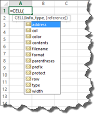
We are going to name our new workbook, so we will choose filename. We will add a sheet name later, but that has to be calculated.
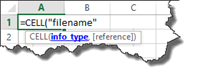
Now we can add reference, which is an optional parameter.
NOTE: If you haven’t noticed yet, optional parameters are always in [].
Enter a closing bracket, then press return.
We see the path to the file.
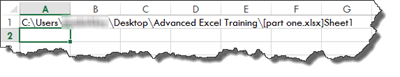
Using the CELL function above, we determined the file path.
Now, we will now create a dynamic formula to extract the sheet name from that path.
To do so, we are going to enter the formula below.

Take note of the different functions we have used.
Now, push Enter. When we do, we see the name of our worksheet displayed in the cell.
If you rename the worksheet in the tab, the worksheet name in the cell will also change.
Next, let’s say we want to see the name of the workbook. We know how to display the path, but we just want to see the file name – or workbook name.
We enter the formula below:

Then push Enter.
Other Information Available in the CELL Function
Here is a list of some of the other information you can choose with the CELL function.
-
COL displays the column number of the referenced cell. You need a cell reference for this. Remember, the cell reference was optional with the workbook name. If you reference cell C3, Excel will display 3. C is the third letter in the alphabet.
-
ROW displays the row number of the referenced cell. Again, you’ll need a cell reference.
-
WIDTH displays the width of the referenced cells in pixels.
-
ADDRESS displays the absolute address of the referenced cell.
-
COLOR displays the value 1 if the referenced cell is formatted in color for negative values. Otherwise, it shows 0.
-
CONTENTS displays the value of the upper left cell in reference.
-
FORMAT displays a text value that corresponds to the number format of the cell. The text value for a percentage format is shown below.
-
PARENTHESES displays a 1 if the referenced cell is formatted with parentheses for positive or all values. Otherwise, it’s 0.
-
PREFIX displays a text value that corresponds to the label prefix of a cell.
-
PROTECT displays a 1 if a cell is locked. Otherwise, it displays a zero.
-
TYPE displays a text value that corresponds to the type of data in a cell. «b» is returned for blank or empty cells. «l» is returned if it contains a text constant. «v» is returned for all other types of cell content.
Here you will find a detailed tutorial on 100+ Excel Functions & VBA Functions. Each Excel function is covered in detail with Examples and Videos.
Excel Functions – Date and Time
| Excel Function | Description |
|---|---|
| Excel DATE Function |
Excel DATE function can be used when you want to get the date value using the year, month and, day values as the input arguments. It returns a serial number that represents a specific date in Excel. |
| Excel DATEVALUE Function |
Excel DATEVALUE function is best suited for situations when a date is stored as text. This function converts the date from text format to a serial number that Excel recognizes as a date. |
| Excel DAY Function |
Excel DAY function can be used when you want to get the day value (ranging between 1 to 31) from a specified date. It returns a value between 0 and 31 depending on the date used as the input. |
| Excel HOUR Function |
Excel HOUR function can be used when you want to get the HOUR integer value from a specified time value. It returns a value between 0 (12:00 A.M.) and 23 (11:00 P.M.) depending on the time value used as the input |
| Excel MINUTE Function |
Excel MINUTE function can be used when you want to get the MINUTE integer value from a specified time value. It returns a value between 0 and 59 depending on the time value used as the input. |
| Excel NETWORKDAYS Function | Excel NETWORKDAYS function can be used when you want to get the number of working days between two given dates. It does not count the weekends between the specified dates (by default the weekend is Saturday and Sunday). It can also exclude any specified holidays. |
| Excel NETWORKDAYS.INTL Function |
Excel NETWORKDAYS.INTL function can be used when you want to get the number of working days between two given dates. It does not count the weekends and holidays, both of which can be specified by the user. It also enables you to specify the weekend (for example, you can specify Friday and Saturday as the weekend, or only Sunday as the weekend). |
| Excel NOW Function | Excel NOW function can be used to get the current date and time value. |
| Excel SECOND Function |
Excel SECOND function can be used want to get the integer value of the seconds from a specified time value. It returns a value between 0 and 59 depending on the time value used as the input. |
| Excel TODAY Function | Excel TODAY function can be used to get the current date. It returns a serial number that represents the current date. |
| Excel WEEKDAY Function |
Excel WEEKDAY function can be used to get the day of the week as a number for the specified date. It returns a number between 1 and 7 that represents the corresponding day of the week. |
| Excel WORKDAY Function |
Excel WORKDAY function can be used when you want to get the date after a given number of working days. By default, it takes Saturday and Sunday as the weekend |
| Excel WORKDAY.INTL Function |
Excel WORKDAY.INTL function can be used when you want to get the date after a given number of working days. In this function, you can specify the weekend to be days other than Saturday and Sunday. |
| Excel DATEDIF Function |
Excel DATEDIF function can be used when you want to calculate the number of years, months, or days between the two specified dates. A good example would be calculating the age. |
Excel Functions – Logical
| Excel Function | Description |
|---|---|
| Excel AND Function |
Excel AND function can be used when you want to check multiple conditions. It returns TRUE only when all the given conditions are true. |
| Excel FALSE Function |
Excel FALSE function returns the logical value FALSE. It does not take any input arguments. |
| Excel IF Function |
Excel IF Function is best suited for situations where you want to evaluate a condition, and the return a value if it is TRUE and another value if it is FALSE. |
| Excel IFS Function |
Excel IFS Function is best suited for situations where you want to test multiple conditions at once and then return the result based on it. This is helpful as you don’t have to create long nested IF formulas that can get confusing. |
| Excel IFERROR Function | Excel IFERROR function is best-suited to handle formula that evaluates to an error. You can specify a value to show if the formula returns an error. |
| Excel NOT Function |
Excel NOT function can be used when you want to reverse the value of a logical argument (TRUE/FALSE). |
| Excel OR Function | Excel OR function can be used when you want to check multiple conditions. It returns TRUE if any of the given condition is true. |
| Excel TRUE Function |
Excel TRUE function returns the logical value TRUE. It does not take any input arguments. |
Excel Functions – Lookup & Reference
| Excel Function | Description |
|---|---|
| Excel COLUMN Function |
Excel COLUMN function can be used when you want to get the column number of a specified cell. |
| Excel COLUMNS Function |
Excel COLUMNS function can be used when you want to get the number of columns in a specified range or array. It returns a number that represents the total number of columns in the specified range or array. |
| Excel HLOOKUP Function |
Excel HLOOKUP function is best suited for situations when you are looking for a matching data point in a row, and when the matching data point is found, you go down that column and fetch a value from a cell which is specified a number of rows below the top row. |
| Excel INDEX Function |
Excel INDEX function can be used when you have the position (row number and column number) of a value in a table, and you want to fetch that value. This is often use with the MATCH function and is a powerful alternative to the VLOOKUP function. |
| Excel INDIRECT Function |
Excel INDIRECT function can be used when you have the references as text and you want to get the values from those references. It returns the reference specified by the text string. |
| Excel MATCH Function |
Excel MATCH function can be used when you want to get the relative position of a lookup value in a list or an array. It returns a number that represents the position of the lookup value in the array. |
| Excel OFFSET Function |
Excel OFFSET function can be used when you want to get a reference which offsets specified number of rows and columns from the starting point. It returns the reference that OFFSET function points to. |
| Excel ROW Function |
Excel ROW Function function can be used when you want to get the row number of a cell reference. For example, =ROW(B4) would return 4, as it is in the fourth row. |
| Excel ROWS Function |
Excel ROWS Function can be used when you want to get the number of rows in a specified range or array. It returns a number that represents the total number of rows in the specified range or array. |
| Excel VLOOKUP Function |
Excel VLOOKUP function is best suited for situations when you are looking for a matching data point in a column, and when the matching data point is found, you go to the right in that row and fetch a value from a cell which is a specified number of columns to the right. |
| Excel XLOOKUP Function |
Excel XLOOKUP function is a new function for Office 365 users and is an enhanced version of the VLOOKUP/HLOOKUP functions. It can be used to lookup and fetch the value in a dataset, and can replace most of what we do with older lookup formulas. |
| Excel FILTER Function |
Excel FILTER function is a new function for Office 365 users that allows you to quickly filter and extract data based on the given condition (or multiple conditions). |
Excel Functions – Math
| Excel Function | Description |
|---|---|
| Excel INT Function |
Excel INT Function can be used when you want to get the integer portion of a number. |
| Excel MOD Function |
Excel MOD function can be used when you want to get the remainder when one number is divided by another. It returns a numerical value that represents the remainder when one number is divided by another. |
| Excel RAND Function |
Excel RAND function can be used when you want to generate evenly distributed random numbers between 0 and 1. It returns a number between 0 and 1 |
| Excel RANDBETWEEN Function |
Excel RANDBETWEEN function can be used when you want to generate evenly distributed random numbers between a top and bottom range specified by the user. It returns a number between the top and bottom range specified by the user. |
| Excel ROUND Function |
Excel ROUND function can be used when you want to return a number rounded to a specified number of digits. |
| Excel SUM Function | Excel SUM function can be used to add all numbers in a range of cells. |
| Excel SUMIF Function |
Excel SUMIF function can be used when you want to add the values in a range if the specified condition is met. |
| Excel SUMIFS Function |
Excel SUMIFS function can be used when you want to add the values in a range if multiple specified criteria are met. |
| Excel SUMPRODUCT Function |
Excel SUMPRODUCT function can be used when you want to first multiply two or more sets to arrays and then get its sum |
Excel Functions – Statistics
| Excel Function | Description |
|---|---|
| Excel RANK Function |
Excel RANK function can be used when you want to rank a number against a list of numbers. It returns a number that represents the relative rank of the number against the list of numbers. |
| Excel AVERAGE Function |
Excel AVERAGE function can be used when you want to get the average (arithmetic mean) of the specified arguments. |
| Excel AVERAGEIF Function |
Excel AVERAGEIF function can be used when you want to get the average (arithmetic mean) of all the values in a range of cells that meet a given criteria. |
| Excel AVERAGEIFS Function |
Excel AVERAGEIFS function can be used when you want to get the average (arithmetic mean) of all the cells in a range that meets multiple criteria. |
| Excel COUNT Function | Excel COUNT function can be used to count the number of cells that contain numbers. |
| Excel COUNTA Function |
Excel COUNTA function can be used when you want to count all the cells in a range that are not empty. |
| Excel COUNTBLANK Function |
Excel COUNTBALNK function can be used when you have to count all the empty cells in a range. |
| Excel COUNTIF Function |
Excel COUNTIF function can be used when you want to count the number of cells that meet a specified criterion. |
| Excel COUNTIFS Function |
Excel COUNTIFS function can be used when you want to count the number of cells that meet a single or multiple criteria. |
| Excel LARGE Function |
Excel LARGE function can be used to get the Kth largest value from a range of cells or array. For example, you can get the third largest value from a range of cells. |
| Excel MAX Function |
Excel MAX function can be used when you want to get the largest value from a set of values. |
| Excel MIN Function |
Excel MIN function can be used when you want to get the smallest value from a set of values. |
| Excel SMALL Function |
Excel SMALL function can be used to get the Kth smallest value from a range of cells or array. For example, you can get the third smallestvalue from a range of cells. |
Excel Functions – Text Functions
| Excel Function | Description |
|---|---|
| Excel CONCATENATE Function |
Excel CONCATENATE function can be used when you want to join 2 or more characters or strings. It can be used to join text, numbers, cell references, or a combination of these. |
| Excel FIND Function |
Excel FIND function can be used when you want to locate a text string within another text string and find its position. It returns a number that represents the starting position of the string you are finding in another string. It is case-sensitive. |
| Excel LEFT Function | Excel LEFT function can be used to extract text from left of the string. It returns the specified number of characters from the left of the string |
| Excel LEN Function |
Excel LEN function can be used when you want to get the total number of characters in a specified string. This is useful when you want to know the length of a string in a cell. |
| Excel LOWER Function |
Excel LOWER function can be used when you want to convert all uppercase letter in a text string to lowercase. Numbers, special characters, and punctuations are not changed by the LOWER function. |
| Excel MID Function |
Excel MID function can be used to extract a specified number of characters from a string. It returns the sub-string from a string. |
| Excel PROPER Function |
Excel PROPER function can be used when you want to capitalize the first character of every word. Numbers, special characters, and punctuations are not changed by the PROPER function. |
| Excel REPLACE Function |
Excel REPLACE function can be used when you want to replace a part of the text string with another string. It returns a text string where a part of the text has been replaced by the specified string. |
| Excel REPT Function |
Excel REPT function can be used when you want to repeat a specified text a certain number of times. |
| Excel RIGHT Function | The RIGHT function can be used to extract text from the right of the string. It returns the specified number of characters from the right of the string |
| Excel SEARCH Function |
Excel SEARCH function can be used when you want to locate a text string within another text string and find its position. It returns a number that represents the starting position of the string you are finding in another string. It is NOT case-sensitive. |
| Excel SUBSTITUTE Function
|
Excel SUBSTITUTE function can be used when you want to substitute text with new specified text in a string. It returns a text string where an old text has been substituted by the new one. |
| Excel TEXT Function |
Excel TEXT function can be used when you want to convert a number to text format and display it in a specified format. |
| Excel TRIM Function | Excel TRIM function can be used when you want to remove leading, trailing, and double spaces in Excel. |
| Excel UPPER Function | Excel UPPER function can be used when you want to convert all lowercase letters in a text string to uppercase. Numbers, special characters, and punctuations are not changed by the UPPER function. |
Excel Functions – Info
| Excel Function | Description |
|---|---|
| Excel ISBLANK Function
Excel ISERROR Function Excel ISNA Function Excel ISNUMBER Function Excel ISEVEN Function Excel ISODD Function Excel ISLOGICAL Function Excel ISTEXT Function |
Excel IS function returns TRUE when specified condition is TRUE. For example, ISNA would return TRUE if the cell has a #N/A! error. |
Excel Functions – Financial
| Excel Function | Description |
|---|---|
| Excel PMT Function | Excel PMT function helps you calculate the payment you need to make for a loan when you know the total loan amount, interest rate, and the number of constant payments. |
| Excel NPV Function | Excel NPV function allows you to calculate the Net Present Value of all the cashflows when you know the discount rate |
| Excel IRR Function | Excel IRR function allows you to calculate the Internal Rate of Return when you have the cashflows data |
VBA Functions
| Excel Function | Description |
|---|---|
| VBA TRIM Function |
VBA TRIM function allows you to remove the leading and trailing spaces from a text string in Excel. It can be a useful VBA function if you want to quickly clean the data. |
| VBA SPLIT Function |
VBA SPLIT function alllows you to split a text string based on the delimiter. For example, if you want to split text based on a comma or tab or colon, you can do that with the SPLIT function. |
| VBA MsgBox Function |
VBA MsgBox is a function that displays a dialog box that you can use to inform your users by showing a custom message or get some basic inputs (such as Yes/No or OK/Cancel). |
| VBA INSTR Function |
VBA InStr function finds the position of a specified substring within the string and returns the first position of its occurrence. |
| VBA UCase Function |
Excel VBA UCASE function takes a string as the input and converts all the lower case characters into upper case. |
| VBA LCase Function |
Excel VBA LCASE function takes a string as the input and converts all the upper case characters into lower case. |
| VBA DIR Function |
Use VBA DIR function when you want to get the name of the file or a folder, using their path name |
Useful Excel Resources:
- 100+ Excel Interview Questions
- 200+ Excel Keyboard Shortcuts
- Free Excel Templates
- Free Online Excel Training
- Best Excel Books
- Excel Formulas Not Working: Possible Reasons and How to FIX IT!
- 20 Advanced Excel Functions and Formulas (for Excel Pros)
- Formula vs Function in Excel – What’s the Difference?
Below is a brief overview of about 100 important Excel functions you should know, with links to detailed examples. We also have a large list of example formulas, a more complete list of Excel functions, and video training. If you are new to Excel formulas, see this introduction.
Note: Excel now includes Dynamic Array formulas, which offer important new functions.
Date and Time Functions
Excel provides many functions to work with dates and times.
NOW and TODAY
You can get the current date with the TODAY function and the current date and time with the NOW Function. Technically, the NOW function returns the current date and time, but you can format as time only, as seen below:

TODAY() // returns current date
NOW() // returns current time
Note: these are volatile functions and will recalculate with every worksheet change. If you want a static value, use date and time shortcuts.
DAY, MONTH, YEAR, and DATE
You can use the DAY, MONTH, and YEAR functions to disassemble any date into its raw components, and the DATE function to put things back together again.

=DAY("14-Nov-2018") // returns 14
=MONTH("14-Nov-2018") // returns 11
=YEAR("14-Nov-2018") // returns 2018
=DATE(2018,11,14) // returns 14-Nov-2018
HOUR, MINUTE, SECOND, and TIME
Excel provides a set of parallel functions for times. You can use the HOUR, MINUTE, and SECOND functions to extract pieces of a time, and you can assemble a TIME from individual components with the TIME function.

=HOUR("10:30") // returns 10
=MINUTE("10:30") // returns 30
=SECOND("10:30") // returns 0
=TIME(10,30,0) // returns 10:30
DATEDIF and YEARFRAC
You can use the DATEDIF function to get time between dates in years, months, or days. DATEDIF can also be configured to get total time in «normalized» denominations, i.e. «2 years and 6 months and 27 days».

Use YEARFRAC to get fractional years:

=YEARFRAC("14-Nov-2018","10-Jun-2021") // returns 2.57
EDATE and EOMONTH
A common task with dates is to shift a date forward (or backward) by a given number of months. You can use the EDATE and EOMONTH functions for this. EDATE moves by month and retains the day. EOMONTH works the same way, but always returns the last day of the month.

EDATE(date,6) // 6 months forward
EOMONTH(date,6) // 6 months forward (end of month)
WORKDAY and NETWORKDAYS
To figure out a date n working days in the future, you can use the WORKDAY function. To calculate the number of workdays between two dates, you can use NETWORKDAYS.

WORKDAY(start,n,holidays) // date n workdays in future
Video: How to calculate due dates with WORKDAY

NETWORKDAYS(start,end,holidays) // number of workdays between dates
Note: Both functions automatically skip weekends (Saturday and Sunday) and will also skip holidays, if provided. If you need more flexibility on what days are considered weekends, see the WORKDAY.INTL function and NETWORKDAYS.INTL function.
WEEKDAY and WEEKNUM
To figure out the day of week from a date, Excel provides the WEEKDAY function. WEEKDAY returns a number between 1-7 that indicates Sunday, Monday, Tuesday, etc. Use the WEEKNUM function to get the week number in a given year.

=WEEKDAY(date) // returns a number 1-7
=WEEKNUM(date) // returns week number in year
Engineering
CONVERT
Most Engineering functions are pretty technical…you’ll find a lot of functions for complex numbers in this section. However, the CONVERT function is quite useful for everyday unit conversions. You can use CONVERT to change units for distance, weight, temperature, and much more.

=CONVERT(72,"F","C") // returns 22.2
Information Functions
ISBLANK, ISERROR, ISNUMBER, and ISFORMULA
Excel provides many functions for checking the value in a cell, including ISNUMBER, ISTEXT, ISLOGICAL, ISBLANK, ISERROR, and ISFORMULA These functions are sometimes called the «IS» functions, and they all return TRUE or FALSE based on a cell’s contents.

Excel also has ISODD and ISEVEN functions that will test a number to see if it’s even or odd.
By the way, the green fill in the screenshot above is applied automatically with a conditional formatting formula.
Logical Functions
Excel’s logical functions are a key building block of many advanced formulas. Logical functions return the boolean values TRUE or FALSE. If you need a primer on logical formulas, this video goes through many examples.
AND, OR and NOT
The core of Excel’s logical functions are the AND function, the OR function, and the NOT function. In the screen below, each of these function is used to run a simple test on the values in column B:

=AND(B5>3,B5<9)
=OR(B5=3,B5=9)
=NOT(B5=2)
- Video: How to build logical formulas
- Guide: 50 examples of formula criteria
IFERROR and IFNA
The IFERROR function and IFNA function can be used as a simple way to trap and handle errors. In the screen below, VLOOKUP is used to retrieve cost from a menu item. Column F contains just a VLOOKUP function, with no error handling. Column G shows how to use IFNA with VLOOKUP to display a custom message when an unrecognized item is entered.

=VLOOKUP(E5,menu,2,0) // no error trapping
=IFNA(VLOOKUP(E5,menu,2,0),"Not found") // catch errors
Whereas IFNA only catches an #N/A error, the IFERROR function will catch any formula error.
IF and IFS functions
The IF function is one of the most used functions in Excel. In the screen below, IF checks test scores and assigns «pass» or «fail»:

Multiple IF functions can be nested together to perform more complex logical tests.
New in Excel 2019 and Excel 365, the IFS function can run multiple logical tests without nesting IFs.

=IFS(C5<60,"F",C5<70,"D",C5<80,"C",C5<90,"B",C5>=90,"A")
Lookup and Reference Functions
VLOOKUP and HLOOKUP
Excel offers a number of functions to lookup and retrieve data. Most famous of all is VLOOKUP:

=VLOOKUP(C5,$F$5:$G$7,2,TRUE)
More: 23 things to know about VLOOKUP.
HLOOKUP works like VLOOKUP, but expects data arranged horizontally:

=HLOOKUP(C5,$G$4:$I$5,2,TRUE)
INDEX and MATCH
For more complicated lookups, INDEX and MATCH offers more flexibility and power:

=INDEX(C5:E12,MATCH(H4,B5:B12,0),MATCH(H5,C4:E4,0))
Both the INDEX function and the MATCH function are powerhouse functions that turn up in all kinds of formulas.
More: How to use INDEX and MATCH
LOOKUP
The LOOKUP function has default behaviors that make it useful when solving certain problems. LOOKUP assumes values are sorted in ascending order and always performs an approximate match. When LOOKUP can’t find a match, it will match the next smallest value. In the example below we are using LOOKUP to find the last entry in a column:

ROW and COLUMN
You can use the ROW function and COLUMN function to find row and column numbers on a worksheet. Notice both ROW and COLUMN return values for the current cell if no reference is supplied:

The row function also shows up often in advanced formulas that process data with relative row numbers.
ROWS and COLUMNS
The ROWS function and COLUMNS function provide a count of rows in a reference. In the screen below, we are counting rows and columns in an Excel Table named «Table1».

Note ROWS returns a count of data rows in a table, excluding the header row. By the way, here are 23 things to know about Excel Tables.
HYPERLINK
You can use the HYPERLINK function to construct a link with a formula. Note HYPERLINK lets you build both external links and internal links:

=HYPERLINK(C5,B5)
GETPIVOTDATA
The GETPIVOTDATA function is useful for retrieving information from existing pivot tables.

=GETPIVOTDATA("Sales",$B$4,"Region",I6,"Product",I7)
CHOOSE
The CHOOSE function is handy any time you need to make a choice based on a number:

=CHOOSE(2,"red","blue","green") // returns "blue"
Video: How to use the CHOOSE function
TRANSPOSE
The TRANSPOSE function gives you an easy way to transpose vertical data to horizontal, and vice versa.

{=TRANSPOSE(B4:C9)}
Note: TRANSPOSE is a formula and is, therefore, dynamic. If you just need to do a one-time transpose operation, use Paste Special instead.
OFFSET
The OFFSET function is useful for all kinds of dynamic ranges. From a starting location, it lets you specify row and column offsets, and also the final row and column size. The result is a range that can respond dynamically to changing conditions and inputs. You can feed this range to other functions, as in the screen below, where OFFSET builds a range that is fed to the SUM function:

=SUM(OFFSET(B4,1,I4,4,1)) // sum of Q3
INDIRECT
The INDIRECT function allows you to build references as text. This concept is a bit tricky to understand at first, but it can be useful in many situations. Below, we are using INDIRECT to get values from cell A1 in 5 different worksheets. Each reference is dynamic. If a sheet name changes, the reference will update.

=INDIRECT(B5&"!A1") // =Sheet1!A1
The INDIRECT function is also used to «lock» references so they won’t change, when rows or columns are added or deleted. For more details, see linked examples at the bottom of the INDIRECT function page.
Caution: both OFFSET and INDIRECT are volatile functions and can slow down large or complicated spreadsheets.
STATISTICAL Functions
COUNT and COUNTA
You can count numbers with the COUNT function and non-empty cells with COUNTA. You can count blank cells with COUNTBLANK, but in the screen below we are counting blank cells with COUNTIF, which is more generally useful.

=COUNT(B5:F5) // count numbers
=COUNTA(B5:F5) // count numbers and text
=COUNTIF(B5:F5,"") // count blanks
COUNTIF and COUNTIFS
For conditional counts, the COUNTIF function can apply one criteria. The COUNTIFS function can apply multiple criteria at the same time:

=COUNTIF(C5:C12,"red") // count red
=COUNTIF(F5:F12,">50") // count total > 50
=COUNTIFS(C5:C12,"red",D5:D12,"TX") // red and tx
=COUNTIFS(C5:C12,"blue",F5:F12,">50") // blue > 50
Video: How to use the COUNTIF function
SUM, SUMIF, SUMIFS
To sum everything, use the SUM function. To sum conditionally, use SUMIF or SUMIFS. Following the same pattern as the counting functions, the SUMIF function can apply only one criteria while the SUMIFS function can apply multiple criteria.

=SUM(F5:F12) // everything
=SUMIF(C5:C12,"red",F5:F12) // red only
=SUMIF(F5:F12,">50") // over 50
=SUMIFS(F5:F12,C5:C12,"red",D5:D12,"tx") // red & tx
=SUMIFS(F5:F12,C5:C12,"blue",F5:F12,">50") // blue & >50
Video: How to use the SUMIF function
AVERAGE, AVERAGEIF, and AVERAGEIFS
Following the same pattern, you can calculate an average with AVERAGE, AVERAGEIF, and AVERAGEIFS.

=AVERAGE(F5:F12) // all
=AVERAGEIF(C5:C12,"red",F5:F12) // red only
=AVERAGEIFS(F5:F12,C5:C12,"red",D5:D12,"tx") // red and tx
MIN, MAX, LARGE, SMALL
You can find largest and smallest values with MAX and MIN, and nth largest and smallest values with LARGE and SMALL. In the screen below, data is the named range C5:C13, used in all formulas.

=MAX(data) // largest
=MIN(data) // smallest
=LARGE(data,1) // 1st largest
=LARGE(data,2) // 2nd largest
=LARGE(data,3) // 3rd largest
=SMALL(data,1) // 1st smallest
=SMALL(data,2) // 2nd smallest
=SMALL(data,3) // 3rd smallest
Video: How to find the nth smallest or largest value
MINIFS, MAXIFS
The MINIFS and MAXIFS. These functions let you find minimum and maximum values with conditions:

=MAXIFS(D5:D15,C5:C15,"female") // highest female
=MAXIFS(D5:D15,C5:C15,"male") // highest male
=MINIFS(D5:D15,C5:C15,"female") // lowest female
=MINIFS(D5:D15,C5:C15,"male") // lowest male
Note: MINIFS and MAXIFS are new in Excel via Office 365 and Excel 2019.
MODE
The MODE function returns the most commonly occurring number in a range:

=MODE(B5:G5) // returns 1
RANK
To rank values largest to smallest, or smallest to largest, use the RANK function:

Video: How to rank values with the RANK function
MATH Functions
ABS
To change negative values to positive use the ABS function.

=ABS(-134.50) // returns 134.50
RAND and RANDBETWEEN
Both the RAND function and RANDBETWEEN function can generate random numbers on the fly. RAND creates long decimal numbers between zero and 1. RANDBETWEEN generates random integers between two given numbers.

=RAND() // between zero and 1
=RANDBETWEEN(1,100) // between 1 and 100
ROUND, ROUNDUP, ROUNDDOWN, INT
To round values up or down, use the ROUND function. To force rounding up to a given number of digits, use ROUNDUP. To force rounding down, use ROUNDDOWN. To discard the decimal part of a number altogether, use the INT function.

=ROUND(11.777,1) // returns 11.8
=ROUNDUP(11.777) // returns 11.8
=ROUNDDOWN(11.777,1) // returns 11.7
=INT(11.777) // returns 11
MROUND, CEILING, FLOOR
To round values to the nearest multiple use the MROUND function. The FLOOR function and CEILING function also round to a given multiple. FLOOR forces rounding down, and CEILING forces rounding up.

=MROUND(13.85,.25) // returns 13.75
=CEILING(13.85,.25) // returns 14
=FLOOR(13.85,.25) // returns 13.75
MOD
The MOD function returns the remainder after division. This sounds boring and geeky, but MOD turns up in all kinds of formulas, especially formulas that need to do something «every nth time». In the screen below, you can see how MOD returns zero every third number when the divisor is 3:

SUMPRODUCT
The SUMPRODUCT function is a powerful and versatile tool when dealing with all kinds of data. You can use SUMPRODUCT to easily count and sum based on criteria, and you can use it in elegant ways that just don’t work with COUNTIFS and SUMIFS. In the screen below, we are using SUMPRODUCT to count and sum orders in March. See the SUMPRODUCT page for details and links to many examples.

=SUMPRODUCT(--(MONTH(B5:B12)=3)) // count March
=SUMPRODUCT(--(MONTH(B5:B12)=3),C5:C12) // sum March
SUBTOTAL
The SUBTOTAL function is an «aggregate function» that can perform a number of operations on a set of data. All told, SUBTOTAL can perform 11 operations, including SUM, AVERAGE, COUNT, MAX, MIN, etc. (see this page for the full list). The key feature of SUBTOTAL is that it will ignore rows that have been «filtered out» of an Excel Table, and, optionally, rows that have been manually hidden. In the screen below, SUBTOTAL is used to count and sum only the 7 visible rows in the table:

=SUBTOTAL(3,B5:B14) // returns 7
=SUBTOTAL(9,F5:F14) // returns 9.54
AGGREGATE
Like SUBTOTAL, the AGGREGATE function can also run a number of aggregate operations on a set of data and can optionally ignore hidden rows. The key differences are that AGGREGATE can run more operations (19 total) and can also ignore errors.
In the screen below, AGGREGATE is used to perform MIN, MAX, LARGE and SMALL operations while ignoring errors. Normally, the error in cell B9 would prevent these functions from returning a result. See this page for a full list of operations AGGREGATE can perform.

=AGGREGATE(4,6,values) // MAX ignore errors, returns 100
=AGGREGATE(5,6,values) // MIN ignore errors, returns 75
TEXT Functions
LEFT, RIGHT, MID
To extract characters from the left, right, or middle of text, use LEFT, RIGHT, and MID functions:

=LEFT("ABC-1234-RED",3) // returns "ABC"
=MID("ABC-1234-RED",5,4) // returns "1234"
=RIGHT("ABC-1234-RED",3) // returns "RED"
LEN
The LEN function will return the length of a text string. LEN shows up in a lot of formulas that count words or characters.

FIND, SEARCH
To look for specific text in a cell, use the FIND function or SEARCH function. These functions return the numeric position of matching text, but SEARCH allows wildcards and FIND is case-sensitive. Both functions will throw an error when text is not found, so wrap in the ISNUMBER function to return TRUE or FALSE (example here).

=FIND("Better the devil you know","devil") // returns 12
=SEARCH("This is not my beautiful wife","bea*") // returns 12
REPLACE, SUBSTITUTE
To replace text by position, use the REPLACE function. To replace text by matching, use the SUBSTITUTE function. In the first example, REPLACE removes the two asterisks (**) by replacing the first two characters with an empty string («»). In the second example, SUBSTITUTE removes all hash characters (#) by replacing «#» with «».

=REPLACE("**Red",1,2,"") // returns "Red"
=SUBSTITUTE("##Red##","#","") // returns "Red"
CODE, CHAR
To figure out the numeric code for a character, use the CODE function. To translate the numeric code back to a character, use the CHAR function. In the example below, CODE translates each character in column B to its corresponding code. In column F, CHAR translates the code back to a character.

=CODE("a") // returns 97
=CHAR(97) // returns "a"
Video: How to use the CODE and CHAR functions
TRIM, CLEAN
To get rid of extra space in text, use the TRIM function. To remove line breaks and other non-printing characters, use CLEAN.

=TRIM(A1) // remove extra space
=CLEAN(A1) // remove line breaks
Video: How to clean text with TRIM and CLEAN
CONCAT, TEXTJOIN, CONCATENATE
New in Excel via Office 365 are CONCAT and TEXTJOIN. The CONCAT function lets you concatenate (join) multiple values, including a range of values without a delimiter. The TEXTJOIN function does the same thing, but allows you to specify a delimiter and can also ignore empty values.

=TEXTJOIN(",",TRUE,B4:H4) // returns "red,blue,green,pink,black"
=CONCAT(B7:H7) // returns "8675309"
Excel also provides the CONCATENATE function, but it doesn’t offer special features. I wouldn’t bother with it and would instead concatenate directly with the ampersand (&) character in a formula.
EXACT
The EXACT function allows you to compare two text strings in a case-sensitive manner.

UPPER, LOWER, PROPER
To change the case of text, use the UPPER, LOWER, and PROPER function

=UPPER("Sue BROWN") // returns "SUE BROWN"
=LOWER("Sue BROWN") // returns "sue brown"
=PROPER("Sue BROWN") // returns "Sue Brown"
Video: How to change case with formulas
TEXT
Last but definitely not least is the TEXT function. The text function lets you apply number formatting to numbers (including dates, times, etc.) as text. This is especially useful when you need to embed a formatted number in a message, like «Sale ends on [date]».

=TEXT(B5,"$#,##0.00")
=TEXT(B6,"000000")
="Save "&TEXT(B7,"0%")
="Sale ends "&TEXT(B8,"mmm d")
More: Detailed examples of custom number formatting.
Dynamic Array functions
Dynamic arrays are new in Excel 365, and are a major upgrade to Excel’s formula engine. As part of the dynamic array update, Excel includes new functions which directly leverage dynamic arrays to solve problems that are traditionally hard to solve with conventional formulas. If you are using Excel 365, make sure you are aware of these new functions:
| Function | Purpose |
|---|---|
| FILTER | Filter data and return matching records |
| RANDARRAY | Generate array of random numbers |
| SEQUENCE | Generate array of sequential numbers |
| SORT | Sort range by column |
| SORTBY | Sort range by another range or array |
| UNIQUE | Extract unique values from a list or range |
| XLOOKUP | Modern replacement for VLOOKUP |
| XMATCH | Modern replacement for the MATCH function |
Video: New dynamic array functions in Excel (about 3 minutes).
Quick navigation
ABS, AGGREGATE, AND, AVERAGE, AVERAGEIF, AVERAGEIFS, CEILING, CHAR, CHOOSE, CLEAN, CODE, COLUMN, COLUMNS, CONCAT, CONCATENATE, CONVERT, COUNT, COUNTA, COUNTBLANK, COUNTIF, COUNTIFS, DATE, DATEDIF, DAY, EDATE, EOMONTH, EXACT, FIND, FLOOR, GETPIVOTDATA, HLOOKUP, HOUR, HYPERLINK, IF, IFERROR, IFNA, IFS, INDEX, INDIRECT, INT, ISBLANK, ISERROR, ISEVEN, ISFORMULA, ISLOGICAL, ISNUMBER, ISODD, ISTEXT, LARGE, LEFT, LEN, LOOKUP, LOWER, MATCH, MAX, MAXIFS, MID, MIN, MINIFS, MINUTE, MOD, MODE, MONTH, MROUND, NETWORKDAYS, NOT, NOW, OFFSET, OR, PROPER, RAND, RANDBETWEEN, RANK, REPLACE, RIGHT, ROUND, ROUNDDOWN, ROUNDUP, ROW, ROWS, SEARCH, SECOND, SMALL, SUBSTITUTE, SUBTOTAL, SUM, SUMIF, SUMIFS, SUMPRODUCT, TEXT, TEXTJOIN, TIME, TODAY, TRANSPOSE, TRIM, UPPER, VLOOKUP, WEEKDAY, WEEKNUM, WORKDAY, YEAR, YEARFRAC
Database Function in Excel (Table of Contents)
- Introduction to Database Function in Excel
- How to Use Database Function in Excel?
Introduction to Database Function in Excel
Excel database functions are designed in such a way that a user can use an Excel database to perform the basic operation on it like Sum, Average, Count, Deviation, etc. The database function is an in-built function in MS Excel that will work only on the proper database or table. These functions can be used with some criteria also.
Syntax:
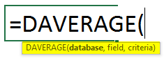
There are some specific in-built Database Functions which are listed below:
- DAVERAGE: It will return the average of the selected database, which is satisfying the user criteria.
- DCOUNT: It will count the cells containing some number in the selected database and satisfy the user criteria.
- DCOUNTA: It will count the non-blank cells in the selected database and which is satisfying the user criteria.
- DGET: It will return a single value from the selected database, which is satisfying the user criteria.
- DMAX: It will return the maximum value of the selected database, which is satisfying the user criteria.
- DMIN: It will return the minimum value of the selected database, which is satisfying the user criteria.
- DPRODUCT: It will return the multiplication output of the selected database, which is satisfying the user criteria.
- DSTDEV: It will return the estimated standard deviation of the population based on the entire population in the selected database, which is satisfying the user criteria.
- DSTDEVP: It will return the standard deviation of the entire population based on the selected database, which is satisfying the user criteria.
- DSUM: It will return the summation of the value from the selected database, which is satisfying the user criteria.
- DVAR: It will return the estimated variance of the population based on the entire population in the selected database, which is satisfying the user criteria.
- DVARP: It will return the Estimates variance of the entire population in the selected database, which is satisfying the user criteria.
How to Use Database Functions in Excel?
Database Functions in Excel is very simple and easy. Let’s understand how to use the Database Functions in Excel with some examples.
You can download this Database Function Excel Template here – Database Function Excel Template
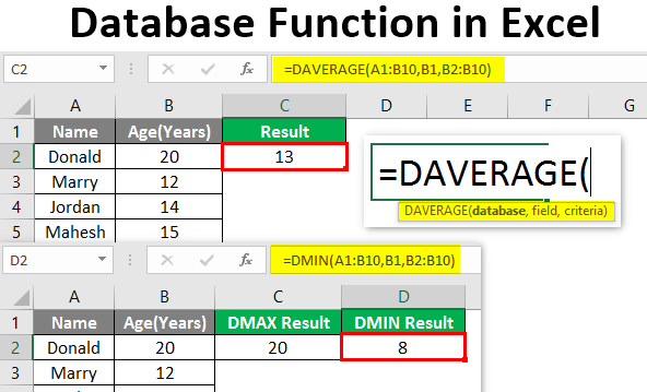
Example #1 – Using DAVERAGE Database Function in Excel
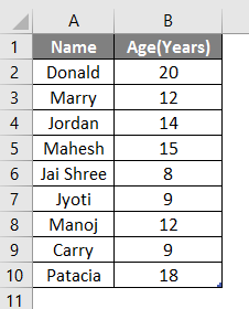
Let’s assume a user has some people’s personal data like Name and Age, where the user wants to calculate the average age of the people in the database. Let’s see how we can do this with the DAVERAGE function.
Open MS Excel from the Start menu, Go to Sheet where the user has kept the data.
Now create headers for DAVERAGE result where we will calculate the average of the people.
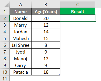
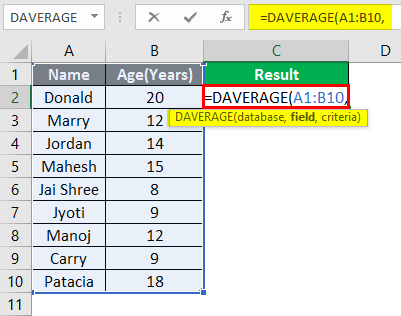
Now calculate the DAVERAGE of the given data by DAVERAGE function, use the equal sign to calculate, Write in C2 Cell.
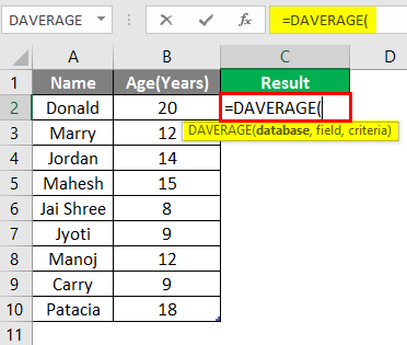
It will then ask for the database given in A1 to B10 cell, select A1 to B10 cell.
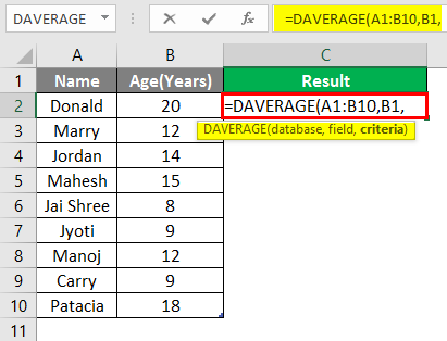
Now it will ask for the Age, so select C1 cell.
It will then ask for criteria from B2 to B10 cell where the condition will be applied and select B2 to B10 cell.
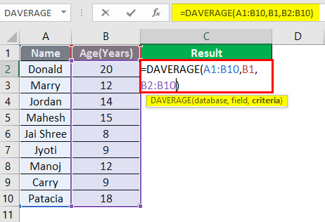
Press the Enter Key.
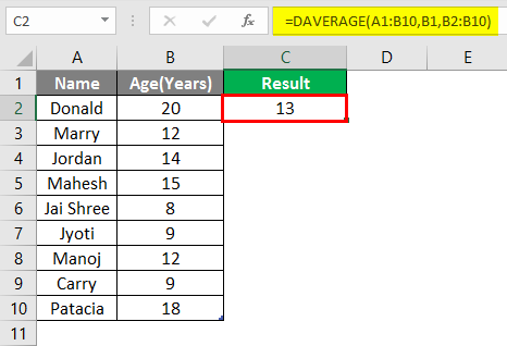
Summary of Example 1: As the user wants to calculate the average age of the people in the database. Everything is calculated in the above excel example, and the Average age is 13 for the group.
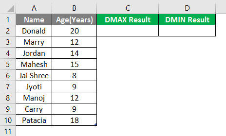
Example #2 – Use of DMAX and DMIN Database Function in Excel
Let’s assume a user has few personal data, like Name and Age, where the user wants to find out the maximum and minimum age of the people in the database. Let’s see how we can do this with the DMAX and DMIN function. Open MS Excel from the Start menu, Go to Sheet where the user kept the data.
Now create headers for DMAX and DMIN results where we will calculate the maximum and minimum age of the people.
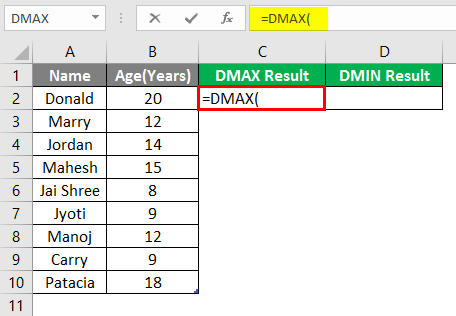
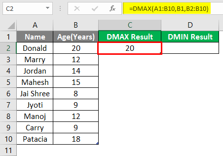
Now calculate the maximum age in the given age data by DMAX function, use the equal sign to calculate, Write in a formula in cell C2.
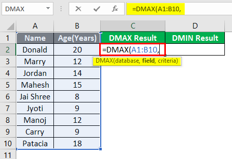
It will then ask for the database given in cell A1 to B10 and select cell A1 to B10.
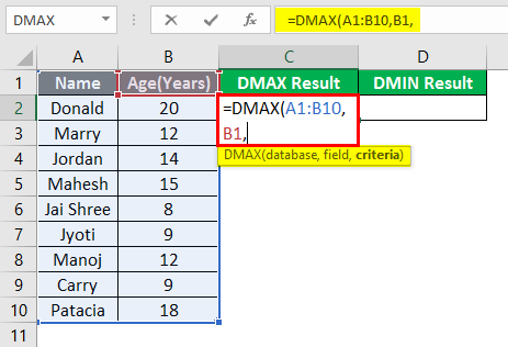
Now it will ask for Age, select B1 cell.
Now it will ask for criteria which are cells B2 to B10 where the condition will be applied, select cell B2 to B10.
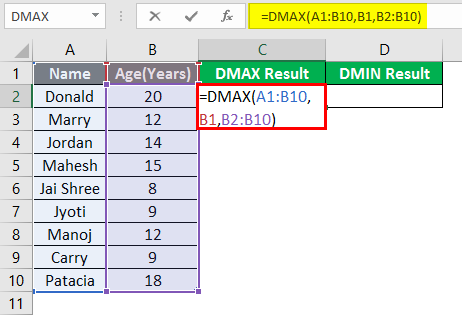
Press the Enter Key.
Now to find out the minimum age, use the DMAX function and follow steps 4 to 7. Use the DMIN formula.
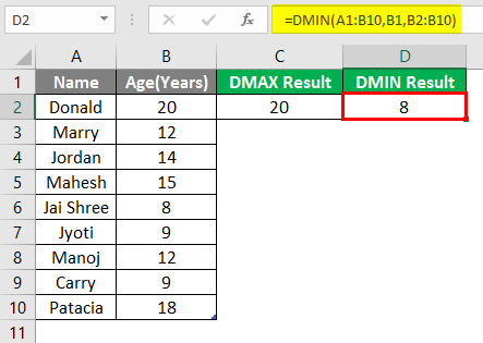
Summary of Example 2: As the user wants to find out the maximum and minimum age of the people in the database. Easley everything calculated in the above excel example and the Maximum age is 20, and the minimum is 8 for the group.
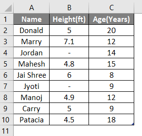
Example #3 – Use of DCOUNT and DCOUNTA Database Function in Excel
A user wants to find out the numeric data count and nonblank cell count in the height column in the database. Let’s see how we can do this with the DCOUNT and DCOUNTA function. Open MS Excel from the Start menu; go to Sheet3, where the user kept the data.
Now create headers for DCOUNT and DCOUNTA results.
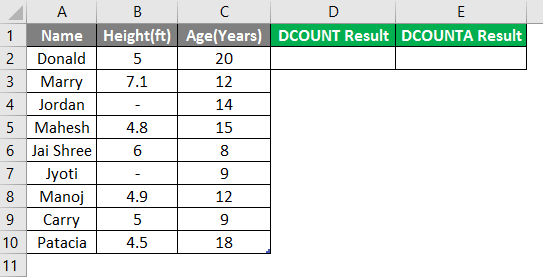
Write the formula in cell D2.
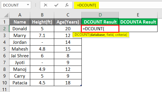
It will then ask for the database given in cell A1 to C10 and select cell A1 to C10.
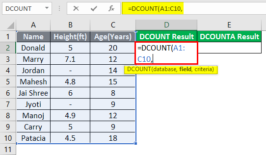
Now it will ask for the Height, select cell B1.
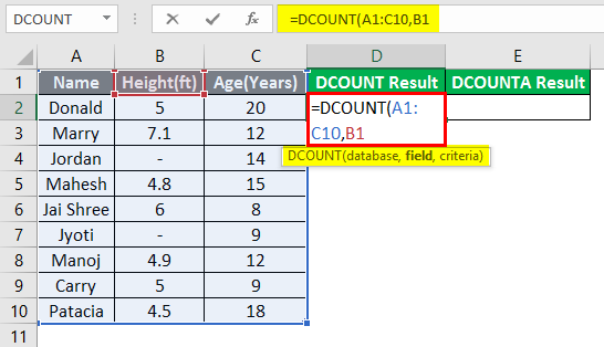
Now it will ask for criteria which are cell B2 to B10, where the condition will be applied, select cell B2 to B10.
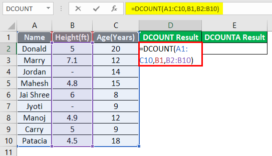
Press Enter key.
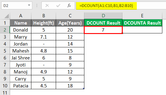
Now to find out nonblank cell function follow steps 4 to 7. Use the DCOUNTA formula.
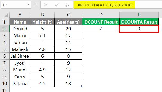
Summary of Example 3: As the user wants to find out the numeric data count and nonblank cell count in the height column. Easley everything calculated in the above excel example, the numeric data count is 7, and the nonblank cell count is 9.
Things to Remember About Database Functions in Excel
- All database functions follow the same syntax, and it has 3 arguments: a database, field, and criteria.
- Database function will work only if the database has a proper table format like it should have a header.
Recommended Articles
This is a guide to Database Function in Excel. Here we discuss how to use Database Function in Excel along with practical examples and downloadable excel template. You can also go through our other suggested articles –
- Excel Create Database
- Excel Database Template
- User-Defined Function in Excel
- PRODUCT Function in Excel