Function for sum in excel

SUM function

The SUM function adds values. You can add individual values, cell references or ranges or a mix of all three.

For example:

=SUM(A2:A10) Adds the values in cells A2:10.
=SUM(A2:A10, C2:C10) Adds the values in cells A2:10, as well as cells C2:C10.

SUM(number1,[number2],…)

Argument name	Description
number1 Required	The first number you want to add. The number can be like 4, a cell reference like B6, or a cell range like B2:B8.
number2-255 Optional	This is the second number you want to add. You can specify up to 255 numbers in this way.

Argument name

Description

number1

Required

The first number you want to add. The number can be like 4, a cell reference like B6, or a cell range like B2:B8.

number2-255

Optional

This is the second number you want to add. You can specify up to 255 numbers in this way.

This section will discuss some best practices for working with the SUM function. Much of this can be applied to working with other functions as well.

The =1+2 or =A+B Method – While you can enter =1+2+3 or =A1+B1+C2 and get fully accurate results, these methods are error prone for several reasons:

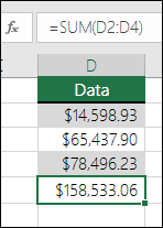
Typos – Imagine trying to enter more and/or much larger values like this:
- =14598.93+65437.90+78496.23
Then try to validate that your entries are correct. It’s much easier to put these values in individual cells and use a SUM formula. In addition, you can format the values when they’re in cells, making them much more readable then when they’re in a formula.
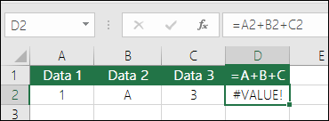
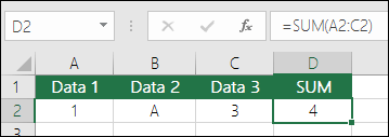
#VALUE! errors from referencing text instead of numbers

If you use a formula like:
- =A1+B1+C1 or =A1+A2+A3
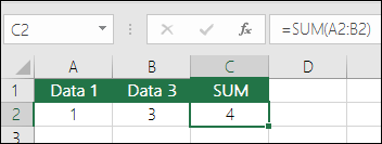
Your formula can break if there are any non-numeric (text) values in the referenced cells, which will return a #VALUE! error. SUM will ignore text values and give you the sum of just the numeric values.
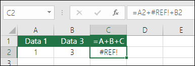
#REF! error from deleting rows or columns

If you delete a row or column, the formula will not update to exclude the deleted row and it will return a #REF! error, where a SUM function will automatically update.
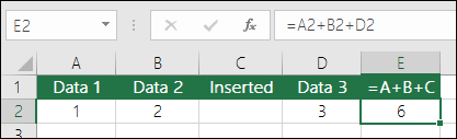
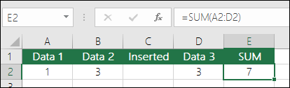
Formulas won’t update references when inserting rows or columns

If you insert a row or column, the formula will not update to include the added row, where a SUM function will automatically update (as long as you’re not outside of the range referenced in the formula). This is especially important if you expect your formula to update and it doesn’t, as it will leave you with incomplete results that you might not catch.
SUM with individual Cell References vs. Ranges

Using a formula like:
- =SUM(A1,A2,A3,B1,B2,B3)
Is equally error prone when inserting or deleting rows within the referenced range for the same reasons. It’s much better to use individual ranges, like:
- =SUM(A1:A3,B1:B3)
Which will update when adding or deleting rows.

I just want to Add/Subtract/Multiply/Divide numbers See this video series on Basic Math in Excel, or Use Excel as your calculator.
How do I show more/less decimal places? You can change your number format. Select the cell or range in question and use Ctrl+1 to bring up the Format Cells Dialog, then click the Number tab and select the format you want, making sure to indicate the number of decimal places you want.
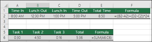
How do I add or subtract Times? You can add and subtract times in a few different ways. For example, to get the difference between 8:00 AM — 12:00 PM for payroll purposes you would use: =(«12:00 PM»-«8:00 AM»)*24, taking the end time minus the start time. Note that Excel calculates times as a fraction of a day, so you need to multiply by 24 to get the total hours. In the first example we’re using =((B2-A2)+(D2-C2))*24 to get the sum of hours from start to finish, less a lunch break (8.50 hours total).

If you’re simply adding hours and minutes and want to display that way, then you can sum and don’t need to multiply by 24, so in the second example we’re using =SUM(A6:C6) since we just need the total number of hours and minutes for assigned tasks (5:36, or 5 hours, 36 minutes).

For more information, see: Add or subtract time.
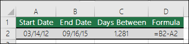
How do I get the difference between dates? As with times, you can add and subtract dates. Here’s a very common example of counting the number of days between two dates. It’s as simple as =B2-A2. The key to working with both Dates and Times is that you start with the End Date/Time and subtract the Start Date/Time.

For more ways to work with dates see: Calculate the difference between two dates.
How do I sum just visible cells? Sometimes, when you manually hide rows or use AutoFilter to display only certain data you also only want to sum the visible cells. You can use the SUBTOTAL function. If you’re using a total row in an Excel table, any function you select from the Total drop-down will automatically be entered as a subtotal. See more about how to Total the data in an Excel table.

Need more help?

You can always ask an expert in the Excel Tech Community or get support in the Answers community.

Советы

Как только вы начнете писать после знака =, Excel покажет выпадающий список доступных функций. Нажмите на функцию, которую хотите использовать, в нашем случае, на SUM.
Представьте, что двоеточие – это слово НА, например, B4 НА B7.

Об этой статье

Эту страницу просматривали 12 332 раза.

Была ли эта статья полезной?

Источник

The SUM function in excel adds the numerical values in a range of cells. Being categorized under the Math and Trigonometry function, it is entered by typing “=SUM” followed by the values to be summed. The values supplied to the function can be numbers, cell references or ranges.

For example, cells B1, B2, and B3 contain 20, 44, and 67 respectively. The formula “=SUM(B1:B3)” adds the numbers of the cells B1 to B3. It returns 131.

The SUM formula automatically updates with the insertion or deletion of a value. It also includes the changes made to an existing cell range. Moreover, the function ignores the empty cells and text values.

SUM Function in Excel
- The Syntax of the SUM Excel Function
- The Procedure to Enter the SUM Function in Excel
- The AutoSum Option in Excel
- How to Use the SUM Function in Excel?
  - Example #1
  - Example #2
  - Example #3
  - Example #4
  - Example #5
- The Usage of the SUM Excel Function
- The Limitations of the SUM Function in Excel
- The Nesting of the SUM Excel Function
- Frequently Asked Questions
- SUM Function in Excel Video
- Recommended Articles

The Syntax of the SUM Excel Function

The syntax of the function is shown in the following image:

The function accepts the following arguments:

Number1: This is the first numeric value to be added.
Number2: This is the second numeric value to be added.

The “number1” argument is required while the subsequent numbers (“number 2”, “number 3”, etc.) are optional.

The Procedure to Enter the SUM Function in Excel

You can download this SUM Function Excel Template here – SUM Function Excel Template

To enter the SUM function manually, type “=SUM” followed by the arguments.

The alternative steps to enter the SUM excel function are listed as follows:

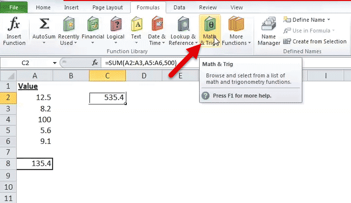
In the Formulas tab, click the “math & trig” option, as shown in the following image.

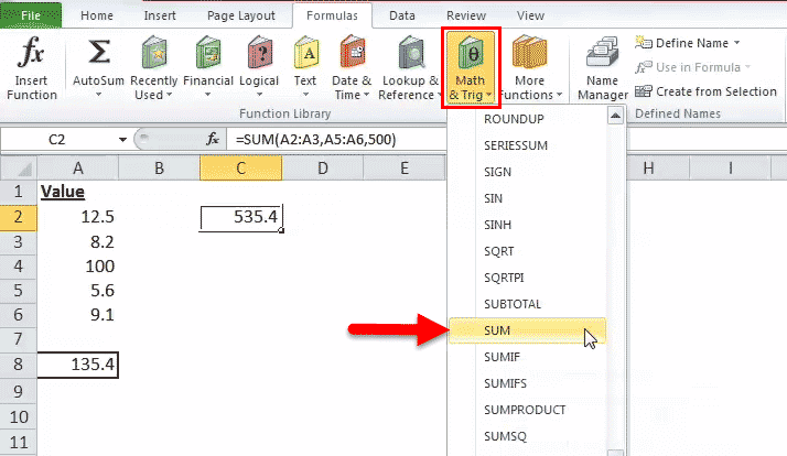
2. From the drop-down menu that opens, select the SUM option.

3. In the “function arguments” dialog box, enter the arguments of the SUM function. Click “Ok” to obtain the output.

The AutoSum Option in Excel

The AutoSum option is the fastest way to add numbers in a range of cells. It automatically enters the SUM formula in the selected cell.

Let us work on an example to understand the working of the AutoSum option. We want to sum the list of values in A2:A7, shown in the succeeding image.

The steps to use the AutoSum command are listed as follows:

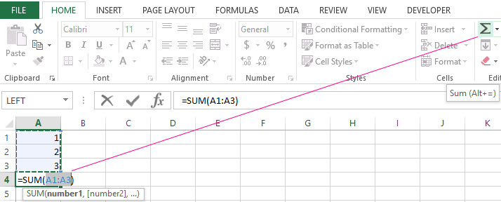
Select the blank cell immediately following the cell to be summed up. Choose the cell A8.
In the Home tab, click “AutoSum”. Alternatively, press the shortcut keys “Alt+=” together and without the inverted commas.
The SUM formula appears in the selected cell. It shows the reference of the cells that have been summed up.
Press the “Enter” key. The output appears in cell A8, as shown in the following image.

How to Use the SUM Function in Excel?

Let us consider a few examples to understand the usage of the SUM function. The examples #1 to #5 show an image containing a list of numeric values.

Example #1

We want to sum the cells A2 and A3 shown in the succeeding image.

Apply the formula “=SUM(A2, A3).” It returns 20.7 in cell C2.

Example #2

We want to sum the cells A3, A5, and the number 45 shown in the succeeding image.

Apply the formula “=SUM (A3, A5, 45).” It returns 58.8 in cell C2.

Example #3

We want to sum the cells A2, A3, A4, A5, and A6 shown in the succeeding image.

Apply the formula “=SUM (A2:A6).” It returns 135.4 in cell C2.

Example #4

We want to sum the cells A2, A3, A5, and A6 shown in the succeeding image.

Apply the formula “=SUM (A2:A3, A5:A6).” It returns 35.4 in cell C2.

Example #5

We want to sum the cells A2, A3, A5, A6, and the number 500 shown in the succeeding image.

Apply the formula “=SUM (A2:A3, A5:A6, 500).” It returns 535.4 in cell C2.

The Usage of the SUM Excel Function

The rules governing the usage of the function are listed as follows:

The arguments supplied can be numbers, arrays, cell references, constants, ranges, and the results of other functions or formulas.
While providing a range of cells, only the first range (cell1:cell2) is required.
The output is numeric and represents the sum of values supplied.
The arguments supplied can go up to a total of 255.

Note: The SUM excel function returns the “#VALUE!” error if the criterion supplied is a text string longer than 255 characters.

The Limitations of the SUM Function in Excel

The drawbacks of the function are listed as follows:

The cell range supplied must match the dimensions of the source.
The cell containing the output must always be formatted as a number.

The Nesting of the SUM Excel Function

The built-in formulas of Excel can be expanded by nesting one or more functions inside another function. This permits multiple calculations to take place in a single cell of the worksheet.

The nested function acts as an argument of the main or the outermost function. Excel calculates the innermost function first and then moves outwards.

For example, the following formula shows the SUM function nested within the ROUND functionThe ROUNDUP excel function calculates the rounded value of the number to the upward side or the higher side. In other words, it rounds the number away from zero. Being an inbuilt function of Excel, it accepts two arguments–the “number” and the “num_of _digits.” For example, “=ROUNDUP(0.40,1)” returns 0.4.
read more:

For the given formula, the output is calculated as follows:

First, the sum of the values in cells A1 to A6 is computed.
Next, the resulting number is rounded to three decimal places.

With Microsoft Excel 2007, nested functions up to 64 levels are permitted. Prior to this version, one could nest functions only till 7 levels.

Frequently Asked Questions

1. Define the SUM function of Excel.

The SUM function helps add the numerical values. These values can be supplied to the function as numbers, cell references, or ranges. The SUM function is used when there is a need to find the total of specified cells.

The syntax of the SUM excel function is stated as follows:
“SUM(number1,[number2] ,…)”
The “number1” and “number2” are the first and second numeric values to be added. The “number1” argument is mandatory while the remaining values are optional.

In the SUM function, the range to be summed can be provided, which is easier than typing the cell references one by one. The AutoSum option provided in the Home or Formulas tab of Excel is the simplest way to sum two numbers.

Note: The numeric value provided as an argument can be either positive or negative.

2. How to sum the values of filtered data in Excel?

To add the values of filtered data, use the SUBTOTAL function. The syntax of the function is stated as follows:

“SUBTOTAL(function_num,ref1,[ref2],…)”

The “function_num” is a number ranging from 1 to 11 or 101 to 111. It indicates the function to be used for the SUBTOTALThe SUBTOTAL excel function performs different arithmetic operations like average, product, sum, standard deviation, variance etc., on a defined range.read more. The functions used can be AVERAGE, MAX, MIN, COUNT, STDEV, SUM, and so on.

The “ref1” and “ref2” are the cells or ranges to be added.

The “function_num” and “ref1” arguments are mandatory. The “function_num” 109 is used for adding the visible cells of filtered data.

Let us consider an example.

• The sales revenue generated by A and B of team X are:
$1,240 and $3,562 given in cells C2 and C3 respectively

• The sales revenue generated by C and D of team Y are:
$2,351 and $4,109 given in cells C4 and C5 respectively

We filter only team X rows and apply the formula “SUBTOTAL(109,C2:C3).” It returns $4,802.

Note: Alternatively, the AutoSum property can be used to sum the filtered cells.

3. State the benefits of using the SUM function in Excel.

The benefits of using the SUM function are listed as follows:
• It helps obtain the totals of ranges irrespective of whether the cells are contiguous or non-contiguous.
• It ignores the empty cells and text values entered in a cell. In such cases, it returns an output representing the sum of the remaining numbers of the range.
• It automatically updates to include the addition of a row or a column.
• It automatically updates to exclude the deletion of a row or column.
• It eliminates the difficulty associated with typing manual entries.
• It makes the output more readable by allowing the cell to be formatted as a number.

SUM Function in Excel Video

Что возвращает функция

Возвращает сумму значений ячеек выбранного диапазона.

Больше лайфхаков в нашем Telegram Подписаться

Синтаксис

=SUM(number1, [number2], …) — английская версия

=СУММ(число1;[число2];…) — русская версия

Аргументы функции

number1 (число1) — первое число, которое вы хотите суммировать. Аргументом может быть также результат вычисления, диапазон ячеек;
[number2] ([число2]) (опционально) — второе число, которое вы хотите суммировать с помощью функции. Оно также может быть диапазоном ячеек или результатом какого-либо вычисления.

Дополнительная информация

Если аргумент функции — массив или ссылка на диапазон ячеек, то, подсчитываются только числа в этом массиве или ссылке. Пустые ячейки, логические значения или текст игнорируются;
Если какой-либо из аргументов является ошибкой, то функция выдаст ошибку.

Примеры использования функции СУММ в Excel

Источник

The SUM function concern into the category «Mathematical». Press the combination of hot keys SHIFT + F3 to call of the function wizard, and you will quickly search out it there.

The using of this function significantly expands to the possibilities of the process of summing the values of the cells in Excel. We look at the possibilities and settings for the summing several ranges practically.

How in the Excel table to calculate the amount of the column?

Sum up the value of the cells A1, A2 and A3 using the summation function and at the same time we will learn what the sum function is used for.

After entering the numbers, go to the cell A4. On the «Home» tab, select the «Sum» tool in the «Edit» section (or press the ALT + = hot keys combination).

The range of the cells is recognized automatically. The reference addresses are already entered in the parameters (A1:A3). The user only remains to press Enter.

Consequently, the calculation result is displayed in the cell A4. The function itself and its parameters can be seen in the formula bar.

The notation. Instead of using the «Sum» tool on the main panel, you can directly enter the function with parameters manually in the cell A4. The result will be the same.

The Automatic Range Recognition Correction

When you enter of the function using the button on the toolbar or using the function wizard (SHIFT + F3), the SUM () function refers to the group of formulas «Mathematical». Automatically recognized ranges are not always suitable for the user: its can be quickly and easily repaired if necessary.

Suppose we need to sum several ranges of cells, as shown in the picture:

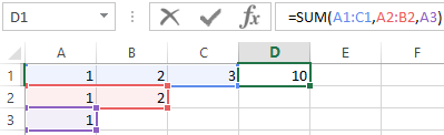
Go to the cell D1 and select the «Sum» tool.
While holding the CTRL key, select the range A2:B2 and the cell A3.
After selecting of the ranges, press Enter and in the cell D4 immediately displays the result of summing the values of cells in all ranges.

Pay attention to the syntax in the function parameters when selecting multiple ranges, that are divided among themselves (;).

In the SUM formula parameters may contain:

the links to individual cells;
the references to ranges of the cells both contiguous and non-adjacent;
the integer and fractional numbers.

In the function parameters, all arguments must be separated by a semicolon.

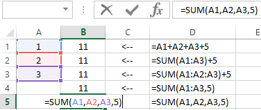
For the illustrative example, let’s consider different variants of summation of values of cells, that give the same result. To do this, fill the cells A1, A2 and A3 with numbers 1, 2 and 3 respectively. And fill the range of the cells B1:B5 with the following formulas and functions:

For any variant, we get the same result of calculation — the number 11. Continue successively with the cursor from B1 and to B5. In each cell, press F2 to see the color highlighting of the links for a more intuitive analysis of the syntax for writing parameters.

The contemporaneous summation of the columns

In Excel, you can simultaneously sum several adjacent and non-adjacent columns.

Fill in the columns, as shown in the picture:

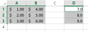
Select the range A1:B3 and holding down the CTRL key also select the column D1:D3.
On the «HOME» panel, click the «Sum» tool (or press ALT + =).

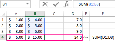
Under each column, the SUM () was automatically added. Now in the cells A4;B4 and D4 the result of the summation of each column is displayed. This is the fastest and most convenient method.

The notation. This function automatically substitutes the format of the cells it sums.

Источник

SUM function

Need more help?

See Also

Need more help?

Want more options?

Советы

Об этой статье

Была ли эта статья полезной?

Table of contents

The Syntax of the SUM Excel Function

The Procedure to Enter the SUM Function in Excel

The AutoSum Option in Excel

How to Use the SUM Function in Excel?

Example #1

Example #2

Example #3

Example #4

Example #5

The Usage of the SUM Excel Function

The Limitations of the SUM Function in Excel

The Nesting of the SUM Excel Function

Frequently Asked Questions

SUM Function in Excel Video

Recommended Articles

Что возвращает функция

Синтаксис

Аргументы функции

Дополнительная информация

Примеры использования функции СУММ в Excel

How in the Excel table to calculate the amount of the column?

The Automatic Range Recognition Correction

The contemporaneous summation of the columns