Function day in excel

This article describes the formula syntax and usage of the DAY function in Microsoft Excel. For information about the DAYS function, see DAYS function.

Description

Returns the day of a date, represented by a serial number. The day is given as an integer ranging from 1 to 31.

Syntax

DAY(serial_number)

The DAY function syntax has the following arguments:

• Serial_number    Required. The date of the day you are trying to find. Dates should be entered by using the DATE function, or as results of other formulas or functions. For example, use DATE(2008,5,23) for the 23rd day of May, 2008. Problems can occur if dates are entered as text.

Remarks

Microsoft Excel stores dates as sequential serial numbers so they can be used in calculations. By default, January 1, 1900 is serial number 1, and January 1, 2008 is serial number 39448 because it is 39,448 days after January 1, 1900.

Values returned by the YEAR, MONTH and DAY functions will be Gregorian values regardless of the display format for the supplied date value. For example, if the display format of the supplied date is Hijri, the returned values for the YEAR, MONTH and DAY functions will be values associated with the equivalent Gregorian date.

Example

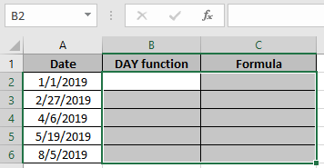
Copy the example data in the following table, and paste it in cell A1 of a new Excel worksheet. For formulas to show results, select them, press F2, and then press Enter. If you need to, you can adjust the column widths to see all the data.

Date
15-Apr-11
Formula	Description (Result)	Result
=DAY(A2)	Day of the date in cell A2 (15)	15

The DAY function has a simple purpose when used by itself. It gives you the «day» component (i.e., a number from 1-31) of a date inside a cell. However, the DAY function allows us to play around with dates in our worksheets by using it with some logical arguments or other functions, as will see in the examples section.

But first, let’s get some basics out of the way.

Syntax

The syntax of the DAY function is as follows:

=DAY(serial_number)

Arguments:

serial_number – The DAY function has just one argument, where you will need to enter a date, either in the form of a serial number or cell reference.

Important Characteristics of the DAY function

• The DAY function extracts the day from a given date and returns it into a cell.
• The DAY function can be nested inside another function to relay the return (for example, in the DATE function).
• If the cell referenced in the serial_number argument does not contain a valid Excel date, the function will return a #VALUE! error.

Examples of the DAY function

Now let’s have a look at some of the examples of the DAY function in Excel.

Example 1 – Plain-vanilla DAY formula

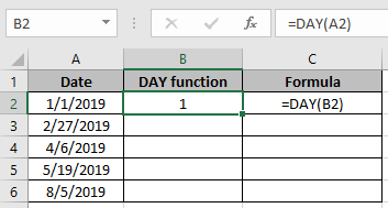
Let’s use the DAY function to extract a day from a date without adding any other complexities. Here is the formula we will use:

=DAY(A2)

No rocket science, right? We have a date in cell A2, and we use the DAY function to extract the day from that date, which is ’25.’

Example 2 – Finding the Number of Days in a Month with DAY function

The formula we will use here is pretty simple. It has a 2-step process and involves 2 functions: DAY and EOMONTH.

We know how the DAY function works. Let’s talk about the EOMONTH function.

The EOMONTH function has 2 arguments. In the first argument, you must supply a date, and in the second argument, you must supply the number of months you want to add to that date.

The EOMONTH function returns the last date of the month, after adding the specified number of months to the given date. For example, if we supply the start date as «12/25/2001» and enter 1 in the second argument, the EOMONTH function will return 01/31/2002.

Alright, now that we have the EOMONTH function covered, let’s look at the formula for finding the number of days in a given month:

=DAY(EOMONTH(A2, 0))

Since our start date is 12/25/2001, the EOMONTH will return 12/31/2001. Also, we know that the DAY function returns the day component of a date, and therefore, it will return ’31,’ i.e. the number of days in December.

Example 3 – Adding Days, Months, or Years with DAY and DATE function

Okay, so let’s say we have a list of dates and a list of days/months/years that we want to add to those dates.

To accomplish this, we will nest the YEAR, MONTH & DAY functions inside the DATE function and add the relevant argument with the corresponding year, month or day to be added. So the formula would be :

=DATE(YEAR(A2) + D2, MONTH(A2) + C2, DAY(A2) + B2)

Essentially, we are trying to add 0 years (from cell D2 to the first argument), 0 months (from cell C2 to the second argument), and 5 days (from cell B2 to the third argument) of the date function. When this formula is dragged down using the fill-handle it populates the correct formula against each row and gives us the suitable output.

Note that instead of putting a number for the years, months, or days to be added in a separate cell, we could just use the number in the formula after the ‘+’ sign instead of referencing the cell.

Example 4 – Fetch the nth Weekday in a Given Month

Let’s say we are trying to find out 2nd and 4th Saturdays in a month, for this we can make use of the DAY and WEEKDAY functions.

We’ll prepare the formula as:

=A2 – DAY(A2) + 1 + n * 7 – WEEKDAY(A2 – DAY(A2) + 8 – 7)

Like we always do, let’s dismantle this formula and understand what each component contributes to the final output.

Step 1

A2 is the start date. From A2, we will subtract the date itself using the DAY function and then add 1.

Why?

Well, all we want to do in this part of the formula is bring the formula to the 1^st day of the month. In our example, cell A2 contains the date 12/22/2001. Removing 22 days using the DAY function, and adding 1, gives us 12/01/2001.

Step 2

Great, so the next component of the formula is n * 7. ‘n’ here is the occurrence of the day in a given month that we want to compute. In our example, we want the 2^nd and 4^th Saturday of the given months, so we will set our n to ‘2’ and ‘4’. In effect, this computation will take us ‘n’ number of weeks into a given month.

We will now continue our discussion with the list of 2^nd Saturdays, but the logic remains the same for both lists.

In step 1, we navigated to the 1^st date of the month. Now, what should we add to this to reach the last day of the nth week? Just the number of weeks multiplied by the number of days in a week, right? So, we will add 14 days (2 * 7) for our list of 2^nd Saturdays.

This brings our formula to 12/15/2001.

Step 3

The final step. Now that we have navigated n number of weeks into a given month, let’s navigate to the specific day we want.

While 12/15/2001 (as computed in Step 2) also happens to be a Saturday, it is the 3^rd Saturday of the month.

So, we will use the WEEKDAY function to backtrack to the intended day. WEEKDAY returns a number from 1 to 7 in which 1 represents a Sunday, and 7 represents a Saturday.

In our example, the WEEKDAY function returns a ‘7.’

Why does WEEKDAY return 7?

The ‘7’ represents the weekday as on the first date in a given month since, within the WEEKDAY function, we navigate to the first day using the DAY function and then add 1.

So, let’s subtract 7 from 12/15/2001 to get our final output.

We get 12/08/2001, which is the 2^nd Saturday; the first Saturday being 12/01/2001.

Example 5 – Get the First Day of the Month with DAY function

I sort of gave this away in the previous example, but let’s quickly recap through how we can compute the first day of the month using the DAY function.

We will use the following formula:

=A2 – DAY(A2) + 1

Does this look familiar? We used this formula in our previous example, too.

A2 is our start day. When we use the DAY function and reference cell A2 in the argument, we are essentially asking it to fetch the day component of the date.

In our example, our start date is December 25, and the DAY function returns 25. Subtracting 25 days from December 25 will give us November 30, so we add 1 and get our final output as 12/01/2001, i.e. the first day of the month.

That’s a wrap on DAY function. When you are done playing around with the DAY function and ace these formulas, we will have another exciting Excel function for you. Until then, keep crunching those numbers.

Функция DAY (ДЕНЬ) используется в Excel, для того чтобы узнать порядковый номер дня месяца (в промежутке от 1 до 31) из любой даты.

Что функция возвращает

Возвращает число в промежутке от 0 до 31, в зависимости от даты, из которой требуется извлечь данные. Например, возвращая данные для Февраля, формула вернет номер дня в промежутке от «0» до «29».

Синтаксис

=DAY(serial_number)

=ДЕНЬ(дата_в_числовом_формате)

Аргументы функции DAY (ДЕНЬ) в Excel

• serial_number (дата_в_числовом_формате): Это порядковый номер дня. Он может быть результатом вычисления формулы, ссылкой на ячейку, которая содержит дату или данные введенные вручную.

Дополнительная информация

Помимо введенных в ручную чисел, функция DAY (ДЕНЬ) также будет работать с:

• результатами вычислений;
• датой введенной в текстовом формате (в кавычках);
• датой, указанной в текстовом формате;
• Excel отразит любую дату начиная с 1 Января 1900 года на Windows и с 1904 года на Mac.

Примеры использования функции DAY (ДЕНЬ) в Excel

Пример №1. Получаем значение дня используя числовой аргумент

На примере выше в качестве аргумента мы используем число “42736”. Это порядковый номер даты “1 января 2017”. Так как 1 января это первый день месяца, то результатом вычисления будет “1”.

Пример №2. Получаем значение дня из ячейки с датой

На примере выше, функция принимает значение ячейки с конкретной датой и возвращает номер дня месяца этой даты. Обратите внимание, что если вы используете формат даты, который не распознается Excel, он покажет ошибку.

Пример №3. Получаем значение дня текущей даты

Вы можете легко получить текущее значение дня с помощью функции TODAY (СЕГОДНЯ) в качестве исходных данных. Функция TODAY (СЕГОДНЯ) возвращает текущую дату, а DAY (ДЕНЬ), в свою очередь, использует эти данные, чтобы вернуть порядковый номер дня этого месяца.

На примере выше, функция TODAY(СЕГОДНЯ) возвращает 12-02-2017. Функция DAY (ДЕНЬ) принимает значение функции TODAY (СЕГОДНЯ) как вводные данные и возвращает значение “12” как порядковый номер дня этого месяца.

Пример №4. Получаем значение первого дня месяца

Вы также можете вычислить значение первого дня любого месяца.

На примере выше, значение дня для даты в ячейке “A2” — “15-03-2017” равно “15”. Для того чтобы узнать номер первого дня месяца этой даты, нам нужно вычесть из нее значение дня (получим “0”, т.к. все даты хранятся в Excel как порядковые номера) и прибавить “1”, чтобы получить первый день месяца.

Обратите внимание, что даты в ячейках D2 и D3 отформатированы как даты. Может случиться так, что, когда вы используете эту формулу, вы можете получить серийный номер (например, “42795” за 1 марта 2017 года). Затем вы можете просто отформатировать его в качестве даты.

Date yes Add (Subtract) Days to a Date Concatenate Dates Convert Date to Number Convert Date to Text Month Name to Number Create Date Range from Dates Day Number of Year Month Name from Date First Day of Month Add (Subtract) Weeks to a Date If Functions with Dates Max Date Number of Days Between Dates Number of Days in a Month Number of Weeks Between Dates Number of Years Between Dates Split Date & Time into Separate Cells Countdown Remaining Days Insert Dates Random Date Generator Using Dynamic Ranges — Year to Date Values Add (Subtract) Years to a Date Date Formula Examples Extract Day from Date Get Day Name from Date Count Days Left in Month / Year Count Workdays Left in Month / Year Get Last Day of Month Last Business Day of Month / Year Number of Work / Business Days in Month Weekday Abbreviations Auto Populate Dates Number of Months Between Dates Quarter from a Date Years of Service Change Date Format Compare Dates Time yes Add (Subtract) Hours to Time Add (Subtract) Minutes to Time Add (Subtract) Seconds to Time Add Up time (Total Time) Time Differences Change Time Format Convert Minutes to Hours Convert Time to Decimal Convert Time to Hours Convert Time to Minutes Convert Time to Seconds Military Time Round Time to Nearest 15 Minutes Overtime Calculator Number of Hours Between Times Convert Seconds to Minutes, Hours, or Time Count Hours Worked Time Differences Time Format — Show Minutes Seconds Text yes Add Commas to Cells Get First Word from Text Capitalize First Letter Clean & Format Phone #s Remove Extra Trailing / Leading Spaces Add Spaces to Cell Assign Number Value to Text Combine Cells with Comma Combine First and Last Names Convert Text String to Date Convert Text to Number Extract Text From Cell Get Last Word Remove Unwated Characters Extract Text Before or After Character How to Split Text String by Space, Comma, & More Remove Special Characters Remove First Characters from Left Substitute Multiple Values Switch First & Last Names w/ Commas Remove Specific Text from a Cell Extract Text Between Characters (Ex. Parenthesis) Add Leading Zeros to a Number Remove Line Breaks from Text Remove all Numbers from Text Reverse Text Remove Non-Numeric Characters Remove Last Character(s) From Right Separate First and Last Names Separate Text & Numbers Round yes Round Formulas Round Price to Nearest Dollar or Cent Round to Nearest 10, 100, or 1000 Round to Nearest 5 or .5 Round Percentages Round to Significant Figures Count yes Count Blank and Non-blank Cells Count Cells Between Two Numbers Count Cells not Equal to Count if Cells are in Range Count Times Word Appears in Cell Count Words in Cell Count Specific Characters in Column Count Total Number of Characters in Column Count Cells that Equal one of two Results Count Cells that do not Contain Count Cells that Contain Specific Text Count Unique Values in Range Countif — Multiple Criteria Count Total Number of Cells in Range Count Cells with Any Text Count Total Cells in a Table Lookup yes Two Dimensional VLOOKUP VLOOKUP Simple Example Vlookup — Multiple Matches Case Sensitive Lookup Case Sensitive VLOOKUP Sum if — VLOOKUP Case Sensitive Lookup Case Sensitive VLOOKUP Find Duplicates w/ VLOOKUP or MATCH INDEX MATCH MATCH Lookup — Return Cell Address (Not Value) Lookup Last Value in Column or Row Reverse VLOOKUP (Right to Left) Risk Score Bucket with VLOOKUP Sum with a VLOOKUP Function VLOOKUP & INDIRECT VLOOKUP Concatenate VLOOKUP Contains (Partial Match) 17 Reasons Why Your XLOOKUP is Not Working Double (Nested) XLOOKUP — Dynamic Columns IFERROR (& IFNA) XLOOKUP Lookup Min / Max Value Nested VLOOKUP Top 11 Alternatives to VLOOKUP (Updated 2022!) VLOOKUP – Dynamic Column Reference VLOOKUP – Fix #N/A Error VLOOKUP – Multiple Sheets at Once VLOOKUP & HLOOKUP Combined VLOOKUP & MATCH Combined VLOOKUP Between Worksheets or Spreadsheets VLOOKUP Duplicate Values VLOOKUP Letter Grades VLOOKUP Return Multiple Columns VLOOKUP Returns 0? Return Blank Instead VLOOKUP w/o #N/A Error XLOOKUP Multiple Sheets at Once XLOOKUP Between Worksheets or Spreadsheets XLOOKUP by Date XLOOKUP Duplicate Values XLOOKUP Multiple Criteria XLOOKUP Return Multiple Columns XLOOKUP Returns 0? Return Blank Instead XLOOKUP Text XLOOKUP with IF XLOOKUP With If Statement Misc. yes Sort Multiple Columns Use Cell Value in Formula Percentage Change Between Numbers Percentage Breakdown Rank Values Add Spaces to Cell CAGR Formula Average Time Decimal Part of Number Integer Part of a Number Compare Items in a List Dealing with NA() Errors Get Worksheet Name Wildcard Characters Hyperlink to Current Folder Compound Interest Formula Percentage Increase Create Random Groups Sort with the Small and Large Functions Non-volatile Function Alternatives Decrease a Number by a Percentage Calculate Percent Variance Profit Margin Calculator Convert Column Number to Letter Get Full Address of Named Range Insert File Name Insert Path Latitute / Longitude Functions Replace Negative Values Reverse List Range Convert State Name to Abbreviation Create Dynamic Hyperlinks Custom Sort List with Formula Data Validation — Custom Formulas Dynamic Sheet Reference (INDIRECT) Reference Cell in Another Sheet or Workbook Get Cell Value by Address Get Worksheet Name Increment Cell Reference List Sheet Names List Skipped Numbers in Sequence Return Address of Max Value in Range Search by Keywords Select Every Other (or Every nth) Row Basics yes Cell Reference Basics — A1, R1C1, 3d, etc. Add Up (Sum) Entire Column or Row Into to Dynamic Array Formulas Conversions yes Convert Time Zones Convert Celsius to Fahrenheit Convert Pounds to Kilograms Convert Time to Unix Time Convert Feet to Meters Convert Centimeters to Inches Convert Kilometers to Miles Convert Inches to Feet Convert Date to Julian Format Convert Column Letter to Number Tests yes Test if a Range Contains any Text Test if any Cell in Range is Number Test if a Cell Contains a Specific Value Test if Cell Contains Any Number Test if Cell Contains Specific Number Test if Cell is Number or Text If yes Percentile If Subtotal If Sumproduct If Large If and Small If Median If Concatentate If Max If Rank If TEXTJOIN If Sum yes Sum if — Begins With / Ends With Sum if — Month or Year to Date Sum if — By Year Sum if — Blank / Non-Blank Sum if — Horizontal Sum Count / Sum If — Cell Color INDIRECT Sum Sum If — Across Multiple Sheets Sum If — By Month Sum If — Cells Not Equal To Sum If — Not Blank Sum if — Between Values Sum If — Week Number Sum Text Sum if — By Category or Group Sum if — Cell Contains Specific Text (Wildcards) Sum if — Date Rnage Sum if — Dates Equal Sum if — Day of Week Sum if — Greater Than Sum if — Less Than Average yes Average Non-Zero Values Average If — Not Blank Average — Ignore 0 Average — Ignore Errors Math yes Multiplication Table Cube Roots nth Roots Square Numbers Square Roots Calculations yes Calculate a Ratio Calculate Age KILLLLLLL Calculate Loan Payments GPA Formula Calculate VAT Tax How to Grade Formulas Find yes Find a Number in a Column / Workbook Find Most Frequent Numbers Find Smallest n Values Find nth Occurance of Character in Text Find and Extract Number from String Find Earliest or Latest Date Based on Criteria Find First Cell with Any Value Find Last Row Find Last Row with Data Find Missing Values Find Largest n Values Most Frequent Number Conditional Formatting yes Conditional Format — Dates & Times Conditional Format — Highlight Blank Cells New Functions XLOOKUP Replaces VLOOKUP, HLOOKUP, and INDEX / MATCH Logical yes AND Checks whether all conditions are met. TRUE/FALSE IF If condition is met, do something, if not, do something else. IFERROR If result is an error then do something else. NOT Changes TRUE to FALSE and FALSE to TRUE. OR Checks whether any conditions are met. TRUE/FALSE XOR Checks whether one and only one condition is met. TRUE/FALSE Lookup & Reference yes FALSE The logical value: FALSE. TRUE The logical value: TRUE. ADDRESS Returns a cell address as text. AREAS Returns the number of areas in a reference. CHOOSE Chooses a value from a list based on it’s position number. COLUMN Returns the column number of a cell reference. COLUMNS Returns the number of columns in an array. HLOOKUP Lookup a value in the first row and return a value. HYPERLINK Creates a clickable link. INDEX Returns a value based on it’s column and row numbers. INDIRECT Creates a cell reference from text. LOOKUP Looks up values either horizontally or vertically. MATCH Searches for a value in a list and returns its position. OFFSET Creates a reference offset from a starting point. ROW Returns the row number of a cell reference. ROWS Returns the number of rows in an array. TRANSPOSE Flips the oriention of a range of cells. VLOOKUP Lookup a value in the first column and return a value. Date & Time yes DATE Returns a date from year, month, and day. DATEDIF Number of days, months or years between two dates. DATEVALUE Converts a date stored as text into a valid date DAY Returns the day as a number (1-31). DAYS Returns the number of days between two dates. DAYS360 Returns days between 2 dates in a 360 day year. EDATE Returns a date, n months away from a start date. EOMONTH Returns the last day of the month, n months away date. HOUR Returns the hour as a number (0-23). MINUTE Returns the minute as a number (0-59). MONTH Returns the month as a number (1-12). NETWORKDAYS Number of working days between 2 dates. NETWORKDAYS.INTL Working days between 2 dates, custom weekends. NOW Returns the current date and time. SECOND Returns the second as a number (0-59) TIME Returns the time from a hour, minute, and second. TIMEVALUE Converts a time stored as text into a valid time. TODAY Returns the current date. WEEKDAY Returns the day of the week as a number (1-7). WEEKNUM Returns the week number in a year (1-52). WORKDAY The date n working days from a date. WORKDAY.INTL The date n working days from a date, custom weekends. YEAR Returns the year. YEARFRAC Returns the fraction of a year between 2 dates. Engineering yes CONVERT Convert number from one unit to another. Financial yes FV Calculates the future value. PV Calculates the present value. NPER Calculates the total number of payment periods. PMT Calculates the payment amount. RATE Calculates the interest Rate. NPV Calculates the net present value. IRR The internal rate of return for a set of periodic CFs. XIRR The internal rate of return for a set of non-periodic CFs. PRICE Calculates the price of a bond. YIELD Calculates the bond yield. INTRATE The interest rate of a fully invested security. Information yes CELL Returns information about a cell. ERROR.TYPE Returns a value representing the cell error. ISBLANK Test if cell is blank. TRUE/FALSE ISERR Test if cell value is an error, ignores #N/A. TRUE/FALSE ISERROR Test if cell value is an error. TRUE/FALSE ISEVEN Test if cell value is even. TRUE/FALSE ISFORMULA Test if cell is a formula. TRUE/FALSE ISLOGICAL Test if cell is logical (TRUE or FALSE). TRUE/FALSE ISNA Test if cell value is #N/A. TRUE/FALSE ISNONTEXT Test if cell is not text (blank cells are not text). TRUE/FALSE ISNUMBER Test if cell is a number. TRUE/FALSE ISODD Test if cell value is odd. TRUE/FALSE ISREF Test if cell value is a reference. TRUE/FALSE ISTEXT Test if cell is text. TRUE/FALSE N Converts a value to a number. NA Returns the error: #N/A. TYPE Returns the type of value in a cell. Math yes ABS Calculates the absolute value of a number. AGGREGATE Define and perform calculations for a database or a list. CEILING Rounds a number up, to the nearest specified multiple. COS Returns the cosine of an angle. DEGREES Converts radians to degrees. DSUM Sums database records that meet certain criteria. EVEN Rounds to the nearest even integer. EXP Calculates the exponential value for a given number. FACT Returns the factorial. FLOOR Rounds a number down, to the nearest specified multiple. GCD Returns the greatest common divisor. INT Rounds a number down to the nearest integer. LCM Returns the least common multiple. LN Returns the natural logarithm of a number. LOG Returns the logarithm of a number to a specified base. LOG10 Returns the base-10 logarithm of a number. MOD Returns the remainder after dividing. MROUND Rounds a number to a specified multiple. ODD Rounds to the nearest odd integer. PI The value of PI. POWER Calculates a number raised to a power. PRODUCT Multiplies an array of numbers. QUOTIENT Returns the integer result of division. RADIANS Converts an angle into radians. RAND Calculates a random number between 0 and 1. RANDBETWEEN Calculates a random number between two numbers. ROUND Rounds a number to a specified number of digits. ROUNDDOWN Rounds a number down (towards zero). ROUNDUP Rounds a number up (away from zero). SIGN Returns the sign of a number. SIN Returns the sine of an angle. SQRT Calculates the square root of a number. SUBTOTAL Returns a summary statistic for a series of data. SUM Adds numbers together. SUMIF Sums numbers that meet a criteria. SUMIFS Sums numbers that meet multiple criteria. SUMPRODUCT Multiplies arrays of numbers and sums the resultant array. TAN Returns the tangent of an angle. TRUNC Truncates a number to a specific number of digits. Stats yes AVERAGE Averages numbers. AVERAGEA Averages numbers. Includes text & FALSE =0, TRUE =1. AVERAGEIF Averages numbers that meet a criteria. AVERAGEIFS Averages numbers that meet multiple criteria. CORREL Calculates the correlation of two series. COUNT Counts cells that contain a number. COUNTA Count cells that are non-blank. COUNTBLANK Counts cells that are blank. COUNTIF Counts cells that meet a criteria. COUNTIFS Counts cells that meet multiple criteria. FORECAST Predict future y-values from linear trend line. FREQUENCY Counts values that fall within specified ranges. GROWTH Calculates Y values based on exponential growth. INTERCEPT Calculates the Y intercept for a best-fit line. LARGE Returns the kth largest value. LINEST Returns statistics about a trendline. MAX Returns the largest number. MEDIAN Returns the median number. MIN Returns the smallest number. MODE Returns the most common number. PERCENTILE Returns the kth percentile. PERCENTILE.INC Returns the kth percentile. Where k is inclusive. PERCENTILE.EXC Returns the kth percentile. Where k is exclusive. QUARTILE Returns the specified quartile value. QUARTILE.INC Returns the specified quartile value. Inclusive. QUARTILE.EXC Returns the specified quartile value. Exclusive. RANK Rank of a number within a series. RANK.AVG Rank of a number within a series. Averages. RANK.EQ Rank of a number within a series. Top Rank. SLOPE Calculates the slope from linear regression. SMALL Returns the kth smallest value. STDEV Calculates the standard deviation. STDEV.P Calculates the SD of an entire population. STDEV.S Calculates the SD of a sample. STDEVP Calculates the SD of an entire population TREND Calculates Y values based on a trendline. Text yes CHAR Returns a character specified by a code. CLEAN Removes all non-printable characters. CODE Returns the numeric code for a character. CONCATENATE Combines text together. DOLLAR Converts a number to text in currency format. EXACT Test if cells are exactly equal. Case-sensitive. TRUE/FALSE FIND Locates position of text within a cell.Case-sensitive. LEFT Truncates text a number of characters from the left. LEN Counts number of characters in text. LOWER Converts text to lower case. MID Extracts text from the middle of a cell. PROPER Converts text to proper case. REPLACE Replaces text based on it’s location. REPT Repeats text a number of times. RIGHT Truncates text a number of characters from the right. SEARCH Locates position of text within a cell.Not Case-sensitive. SUBSTITUTE Finds and replaces text. Case-sensitive. TEXT Converts a value into text with a specific number format. TRIM Removes all extra spaces from text. UPPER Converts text to upper case. VALUE Converts a number stored as text into a number.

How to Use the DAY function in Excel

Get the day of a date in numeric form

What to Know

• Syntax for function: DAY(serial_number).
• Enter date in spreadsheet > select cell > select Formulas > Date & Time > DAY > Serial_number > choose cell.
• If not working, select date column > right-click and select Format Cells > Number tab > Number > OK.

This article explains how to use the DAY function in Microsoft Excel to return a date as a serial number using an integer between 1 and 31.

How to Use the DAY function in Excel 

The syntax for the DAY function is DAY(serial_number).

The only argument for the DAY function is serial_number, which is required. This serial number field refers to the date of the day you are trying to find.

Dates are serial numbers in Excel’s internal system. Beginning with January 1, 1900 (which is number 1), each serial number is assigned in ascending numerical order. For example, January 1, 2008 is serial number 39448 because it is 39447 days after January 1, 1900.

Excel uses the serial number entered to determine which day of the month the date falls on. The day is returned as an integer ranging from 1 to 31.

1. Enter a date in an Excel spreadsheet using the DATE function. You can also use dates appearing as the result of other formulas or functions.

   If dates are entered as text, the DAY function might not work as it should.

2. Select the cell where you want the day of the date to appear.

3. Select Formulas. In Excel Online, select the Insert Function button next to the formula bar to open the Insert Function dialog box.

4. Select Date & Time to open the Function drop-down list. In Excel Online, choose Date & Time in the Pick a Category list. 

5. Select DAY in the list to bring up the function’s dialog box.

6. Make sure the Serial_number field is selected and then choose the cell containing the date you want to use.

7. Choose OK to apply the function and view the number representing the day of the date.

DAY Function Not Working

If your results are not appearing as numbers but rather as dates, it is likely a simple formatting issue. Problems could occur if the numbers are formatted as text rather than dates. Checking the format for the cells containing the serial number portion of the DAY function syntax (and then changing the format, if necessary) is the most likely way to resolve an error or incorrect result.

1. Select the column containing the dates.

2. Right-click anywhere on the selected cells and select Format Cells.

3. Make sure the Number tab is selected and choose Number in the Category list.

4. Select OK to apply the changes and close the dialog. Your results will appear as integers instead of dates.

When to Use the DAY Function in Excel

The DAY function is useful for financial analysis, primarily in a business setting. For instance, a retail organization might want to determine what day of the month has the highest number of customers or when most shipments arrive.

You can also extract a value using the DAY function inside of a larger formula. For instance, in this sample worksheet, the DAY function helps determine how many days are in the listed months.

The formula entered in cell G3 is

=DAY(EOMONTH(F3,0))

The DAY function provides the day component and EOMONTH (end of month) gives you the last day of the month for that date. The syntax for EOMONTH is EOMONTH(start_date, months). So the start date argument is the DAY entry and the number of months is 0, resulting in a list showing the number of days in the months presented.

Be careful not to confuse the DAY function with the DAYS function. The DAYS function, which uses the syntax DAYS(end_date, start_date) returns the number of days between a start date and an end date.

Thanks for letting us know!

Get the Latest Tech News Delivered Every Day

Subscribe

In this article, we will learn about the DAY function in Excel.

DAY function in Excel returns just the number from 1-31 corresponding to the date in the argument.

Syntax:

=DAY(date)

Note: Date should be a valid date

Let’s understand this function using the example shown below
Here we have dates. We will use the function on the below shown data set.

Use the Formula:

=DAY(A2)

Note: Date should be a valid date

As you can see in the above snapshot, we have a date as a number from the date.

Copy the formula in the remaining cells to get the new amount for the rest of the data.

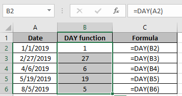
Date(value) can be extracted using the above procedure

Hope you understood how to use the DAY function in Excel. Explore more articles on Mathematical formulation in Excel here. Mention your queries in the comment box below. We will help you with it.

Related Articles:

How to Use TODAY Function in Excel

How to use the Excel TIME function

How to use the NOW Function in Excel

How to use the WEEKDAY Function in Excel

How to use the MONTH Function in Excel

How to Use the YEAR Function in Excel

Popular Articles:

The VLOOKUP Function in Excel

COUNTIF in Excel 2016

How to Use SUMIF Function in Excel

Функция

ДЕНЬ()

, английский вариант DAY(),

возвращает день, соответствующий заданной дате. День определяется как целое число в диапазоне от 1 до 31.

Синтаксис функции

ДЕНЬ

(

дата

)

Дата

— дата, день которой необходимо найти.

Примеры

Используемая в качестве аргумента Дата должна быть в формате воспринимаемым EXCEL. Следующие формулы будут работать:

=ДЕНЬ(«28.02.2011») =ДЕНЬ(«28/02/2011») =ДЕНЬ(«28-02-2011») =ДЕНЬ(«28-фев-2011») =ДЕНЬ(«28-февраль-2011») =ДЕНЬ(«28 февраль 2011») =ДЕНЬ(«2011.02.28»)

=ДЕНЬ(40602)

В EXCEL даты хранятся в виде последовательности чисел (1, 2, 3, …), что позволяет выполнять над ними вычисления. По умолчанию день 1 января 1900 г. имеет номер 1, а 28 февраля 2011 г. — номер 40602, так как интервал между этими датами составляет 40 602 дня. О том как EXCEL хранит дату и время, читайте эту

статью

.

=ДЕНЬ(A1)

Если в ячейке

А1

введена дата в одном из вышеуказанных форматов, то формулой будет возвращен день (28).

Следующие формулы вернут ошибку #ЗНАЧ!

=ДЕНЬ(«28-февраля-2011») =ДЕНЬ(«28 02 2011»)

Использование с функцией

ДАТА()

Для того, чтобы прибавить к дате 28.02.2011, содержащейся в ячейке

А1

, например, 5 лет, можно использовать следующую формулу:

=ДАТА(ГОД(A1)+5;МЕСЯЦ(A1);ДЕНЬ(A1)).