
Split text into different columns with the Convert Text to Columns Wizard
Take text in one or more cells and split it into multiple cells using the Convert Text to Columns Wizard.

Try it!
-
Select the cell or column that contains the text you want to split.
-
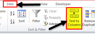
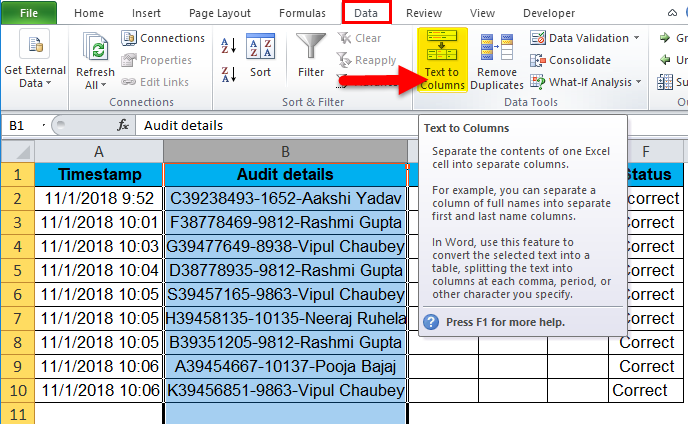
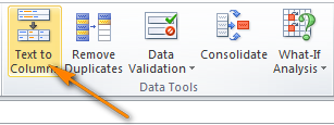
Select Data > Text to Columns.
-
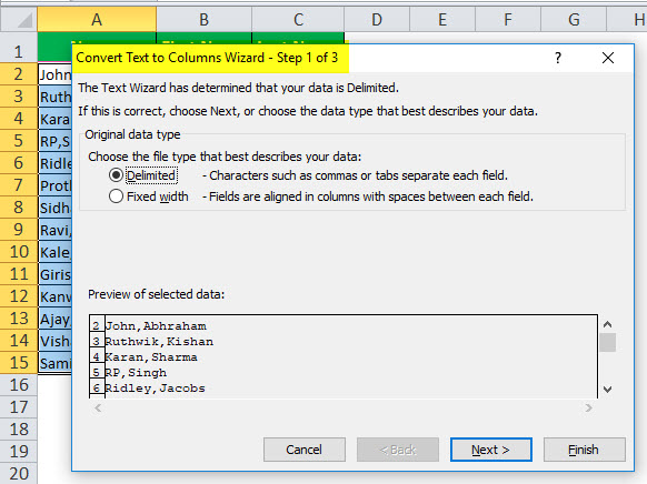
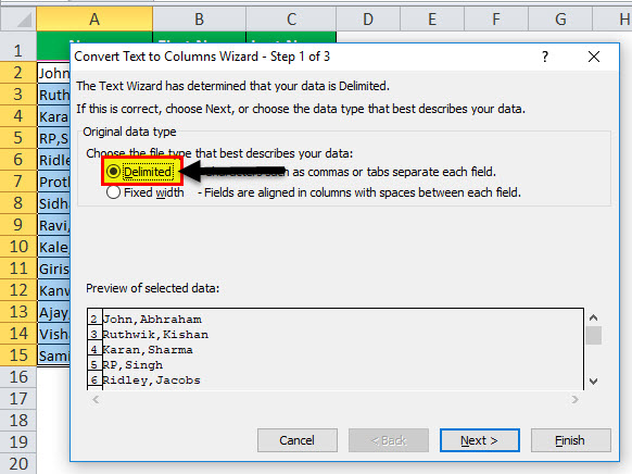
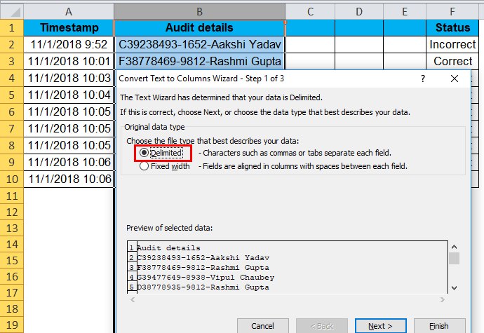
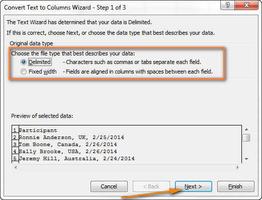
In the Convert Text to Columns Wizard, select Delimited > Next.
-
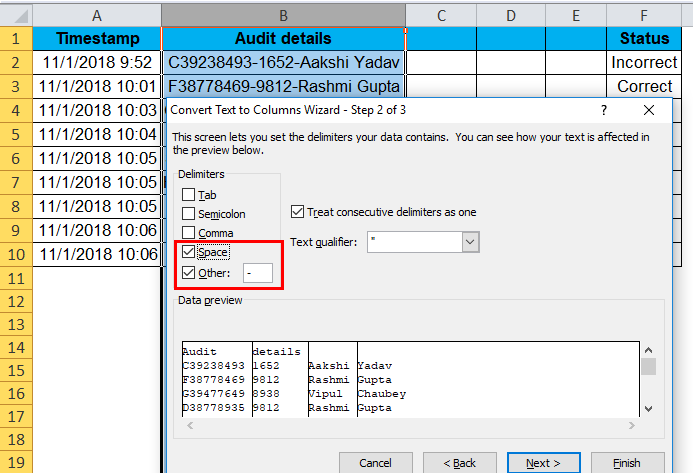
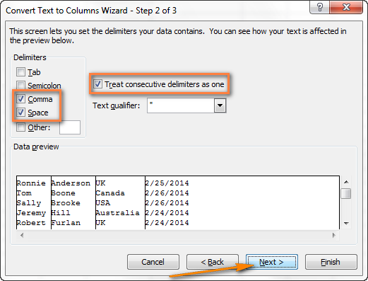
Select the Delimiters for your data. For example, Comma and Space. You can see a preview of your data in the Data preview window.
-
Select Next.
-
Select the Destination in your worksheet which is where you want the split data to appear.
-
Select Finish.
Want more?
Split text into different columns with functions
Need more help?
Want more options?
Explore subscription benefits, browse training courses, learn how to secure your device, and more.
Communities help you ask and answer questions, give feedback, and hear from experts with rich knowledge.
Text to Columns is an amazing feature in Excel that deserves a lot more credit than it usually gets.
As it’s name suggests, it is used to split the text into multiple columns. For example, if you have a first name and last name in the same cell, you can use this to quickly split these into two different cells.
This can be really helpful when you get your data from databases or you import it from other file formats such as Text or CSV.
In this tutorial, you’ll learn about many useful things that can be done using Text to Columns in Excel.
Where to Find Text to Columns in Excel
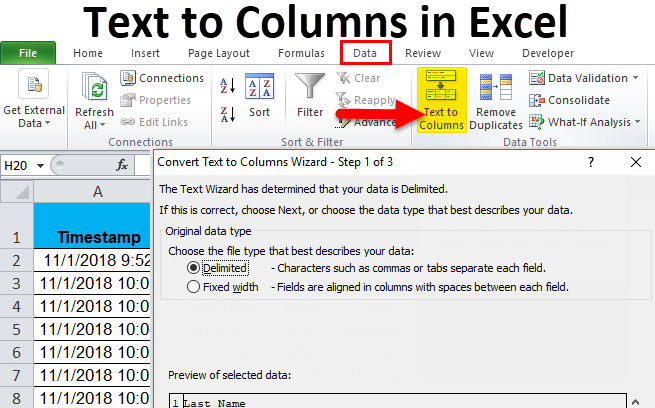
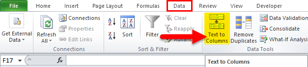
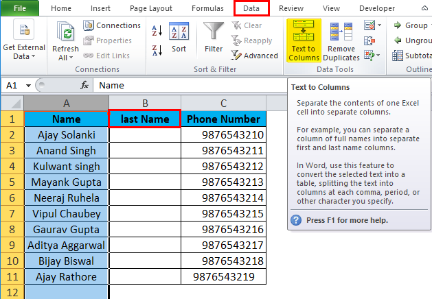
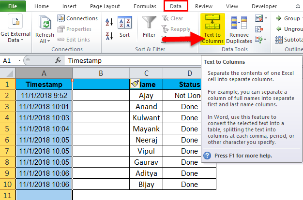
To access Text to Columns, select the dataset and go to Data → Data Tools → Text to Columns.

This would open the Convert Text to Columns Wizard.
This wizard has three steps and takes some user inputs before splitting the text into columns (you will see how these different options can be used in examples below).
To access Text to Columns, you can also use the keyboard shortcut – ALT + A + E.
Now let’s dive in and see some amazing stuff you can do with Text to Columns in Excel.
Example 1 – Split Names into the First Name and Last Name
Suppose you have a dataset as shown below:

To quickly split the first name and the last name and get these in separate cells, follow the below steps:
This would instantly give you the results with the first name in one column and last name in another column.

Note:
- This technique works well when you the name constitutes of the first name and the last name only. In case there are initials or middle names, then this might not work. Click here for a detailed guide on how to tackle cases with different combinations of names.
- The result you get from using the Text to Columns feature is static. This means that if there are any changes in the original data, you’ll have to repeat the process to get updated results.
Also read: How to Sort by the Last Name in Excel
Example 2 – Split Email Ids into Username and Domain Name
Text to Columns allows you to choose your own delimiter to split text.
This can be used to split emails addresses into usernames and domain names as these are separated by the @ sign.
Suppose you have a dataset as shown below:

These are some fictional email ids of some cool superheroes (except myself, I am just a regular wasting-time-on-Netflix kinda guy).
Here are the steps to split these usernames and domain names using the Text to Columns feature.
This would split the email address and give you the first name and the last name in separate cells.

Example 3 – Get the Root Domain from URL
If you work with web URLs, you may sometimes need to know the total number of unique root domains.
For example, in case of http://www.google.com/example1 and http://google.com/example2, the root domain is the same, which is www.google.com
Suppose you have a dataset as shown below:

Here are the steps to get the root domain from these URLs:
This would split the URL and give you the root domain (in the third column as there were two forward slashes before it).

Now if you want to find the number of unique domains, just remove the duplicates.
Note: This works well when you have all the URLs that have http:// in the beginning. If it doesn’t, then you will get the root domain in the first column itself. A good practice is to make these URLs consistent before using Text to Columns.
Example 4 – Convert Invalid Date Formats Into Valid Date Formats
If you get your data from databases such as SAP/Oracle/Capital IQ, or you import it from a text file, there is a possibility that the date format is incorrect (i.e., a format that Excel does not consider as date).
There are only a couple of formats that Excel can understand, and any other format needs to be converted into a valid format to be used in Excel.
Suppose you have dates in the below format (which are not in the valid Excel date format).

Here are the steps to convert these into valid date formats:
This would instantly convert these invalid date formats into valid date formats that you can use in Excel.
Example 5 – Convert Text to Numbers
Sometimes when you import data from databases or other file formats, the numbers are converted into text format.
There are several ways this can happen:
- Having an apostrophe before the number. This leads to the number being treated as text.
- Getting numbers as a result of text functions such as LEFT, RIGHT, or MID.
The problem with this is that these numbers (which are in text format) are ignored by Excel functions such as SUM and AVERAGE.
Suppose you have a dataset as shown below where the numbers are in the text format (note that these are aligned to the left).

Here are the steps to use Text to Columns to convert text to numbers
This would convert these numbers back into General format that can now be used in formulas.
Example 6 – Extract First five Characters of a String
Sometimes you may need to extract the first few characters of a string. These could be the case when you have transactional data and the first five characters (or any other number of characters) represent a unique identifier.
For example, in the data set shown below, the first five characters are unique to a product line.

Here are the steps to quickly extract the first five characters from this data using Text to Columns:
This would split your data set and give you the first five characters of each transaction id in one column and rest all in the second column.

Note: You can set more than one vertical line as well to split the data into more than 2 columns. Just click anywhere in the Data Preview area and drag the cursor to set the divider.
Example 7 – Convert Numbers with Trailing Minus Sign to negative numbers
While this is not something that may encounter often, but sometimes, you may find yourself fixing the numbers with trailing minus signs and making these numbers negative.
Text to Columns is the perfect way to get this sorted.
Suppose you have a dataset as shown below:

Here are the steps to convert these trailing minuses into negative numbers:
This would instantly place the minus sign from the end of the number of the beginning of it. Now you can easily use these numbers in formulas and calculations.
You May Also Like the Following Excel Tutorials:
- CONCATENATE Excel Ranges (with and without separator)
- Excel AUTOFIT: Make Rows/Columns Fit the Text Automatically
- How to Transpose Data in Excel.
- How to Split Cells in Excel.
- How to Merge Cells in Excel the Right Way.
- How to Find Merged Cells in Excel (and get rid of it)
- How to Remove Time from Date in Excel
- How to Convert Text to Date in Excel
Text to columns in Excel is a method that is used to separate a text into different columns based on some delimited or any fixed width. There are two options to use text to columns in Excel. One is using a delimiter where we provide a delimiter as an input such as comma space or hyphen, or we can use a fixed defined width to separate a text in the adjacent columns.
Table of contents
- Excel Text to Columns
- Where to Find Text to Columns Option in Excel?
- How to Split Text to Columns in Excel? (with Examples)
- Examples #1: Split First Name and Last Name
- Examples 2: Convert Single Column Data into Multiple Columns
- Examples 3: Convert Date to Text Using Text to Column Option
- Examples 4: Extract First 9 Characters from the list
- Recommended Articles
Where to Find Text to Columns Option in Excel?
To access text to columns in Excel, go to the Data tab, then Data Tools and Text to Columns.
The keyboard shortcut to open text to columns is – ALT + A + E.
How to Split Text to Columns in Excel? (with Examples)
You can download this Text to Columns Excel Template here – Text to Columns Excel Template
Examples #1: Split First Name and Last Name
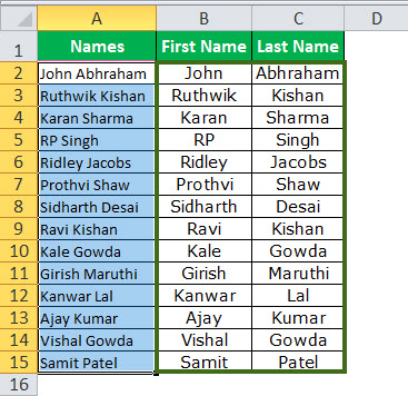
Assume you have a list of names that includes both first and last names in a single column.
You can download this Text to Columns Excel Template here – Text to Columns Excel Template
Now, you need to split the first name and last nameSplit Name in Excel refers to separating the names into two distinct columns. It splits the whole name into First Name, Last Name, and Middle Name. We can separate names using several ways such as the «Text to Column technique» and the «Formula technique.read more separately.
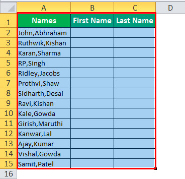
We need to split the first and last names and get these in separate cells.
Below are the steps for splitting first name and last name into separate cells:
- Select the data.

- Then, press “ALT + A +E.” It will open the “Convert Text to Columns Wizard.”

- Now, make sure “Delimited” is selected and click on “Next.”
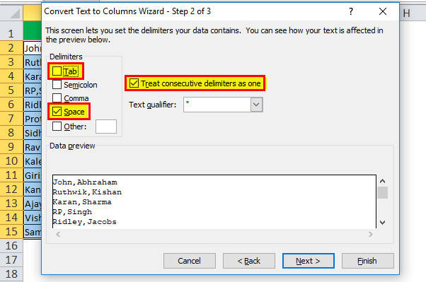
- In the next step, uncheck “TAB” and select “SPACE” as the delimiter. If you think of double/triple consecutive spaces between the names, choose the “Treat consecutive delimiters as one” option. Finally, click on “Next.”

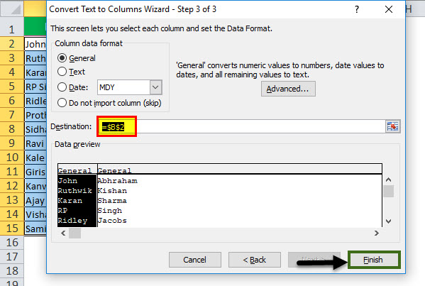
- Select the destination cell. If you do not select a destination cell, it will overwrite the existing data set with the first name in the first column and the last name in the adjacent column. If you want to keep the original data intact, create a copy or choose a different destination cell.

- Click on “FINISH.” That will split the first name and last name separately.

Note: This technique is ideal only for first names and last names. You need to use a different approach if there are initials and middle names.

Examples 2: Convert Single Column Data into Multiple Columns
Let us see how to split the data into multiple columns. It is also part of data cleaning. Sometimes your data is in one single column. You need to divide it into multiple adjacent columns.
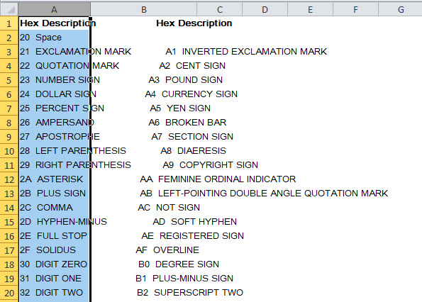
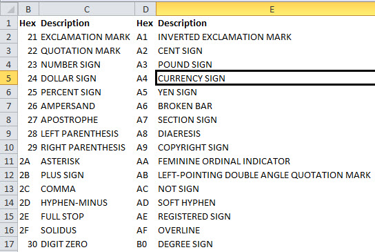
The below data is in one column, and you need to convert it into 4 columns based on the heading.
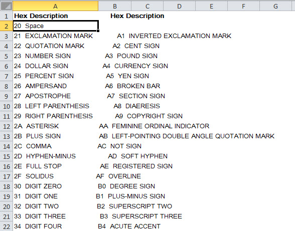
From the above data, we can understand that there are four pieces of information in a single cell: “Hex No., Description,” “Hex No., Description.” Therefore, we will apply the “fixed-width” text to the columns method.
- Step 1: Select the data range.
- Step 2: Go to the “Data” tab and select the “Text to Column” Excel option (ALT + A + E). It would open up the “Convert Text to Columns Wizard” window.
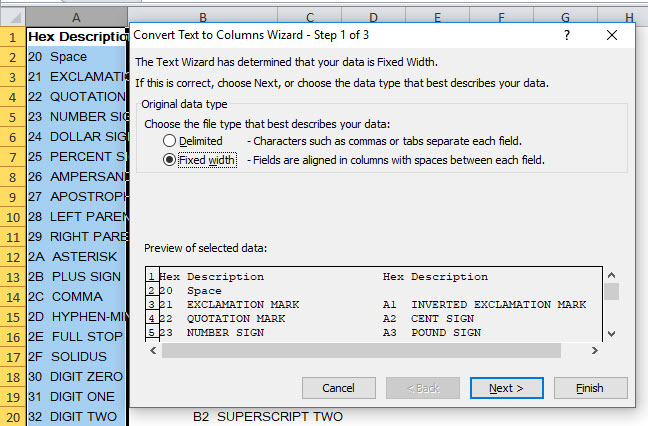
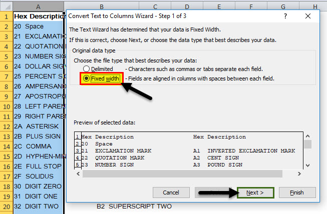
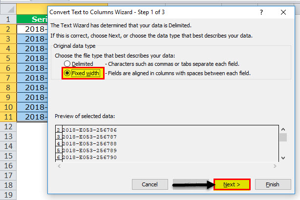
- Step 3: Select the “Fixed width” option and click on “Next.”
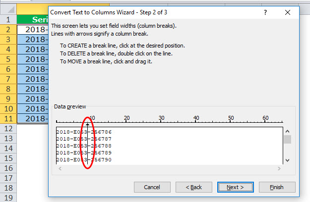
- Step 4: The fixed-width divider vertical line marks (called break line) in the “Data preview” window. You may need to adjust it as per your data structure.

- Step 5: Click on the “Next” option and select the destination cell as B1 in the next option. It would insert the data in the new column to have our original data.
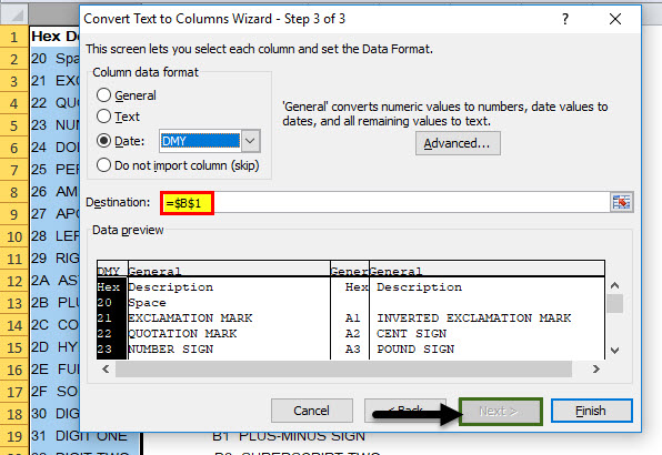
- Step 6: Now, click on the “Finish” button. It would instantly split data into four columns: “Hex,” “Description,” “Hex,” and “Description,” starting from column B to column E.
Examples 3: Convert Date to Text Using Text to Column Option
If you do not like formulas to convert the date to text format, you can use TEXT TO COLUMN Excel OPTION. For example, assume you have data from cells A2 to A8.

Now, you need to convert it into text format.
- Step 1: Select the entire column you want to convert.

- Step 2: Go to the Data tab and Text to Columns.
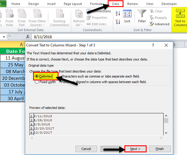
- Step 3: Make sure Delimited is selected and click on the “Next” button.
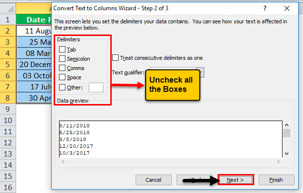
- Step 4: The below pop-up will open, uncheck all the boxes, and click the “Next” button.
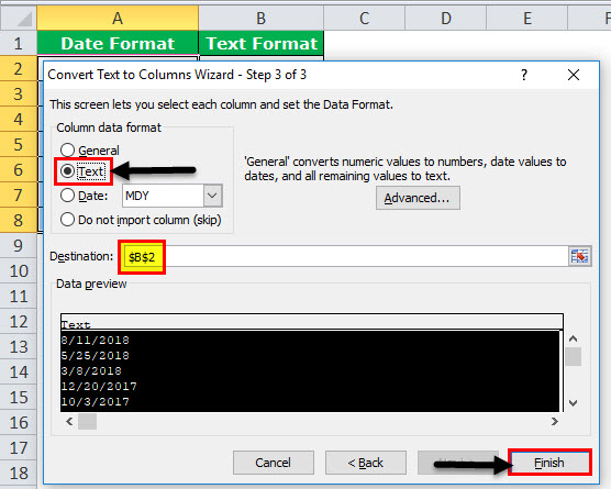
- Step 5: Select the TEXT option from the next dialog box. Mention the destination cell as B2 and click “Finish.”
- Step 6: Now, it instantly converts it into text format.

For example, in the data set shown below, the first 9 characters are unique to a product lineProduct Line refers to the collection of related products that are marketed under a single brand, which may be the flagship brand for the concerned company. Typically, companies extend their product offerings by adding new variants to the existing products with the expectation that the existing consumers will buy products from the brands that they are already purchasing.read more.

- Step 1: Select the data range.

- Step 2: Press “ALT + A + E,” select the “Fixed width,” and click on “Next.”
- Step 3: Now, put a delimiter exactly after the 9th character, as shown in the image below.
- Step 4: Click “Next” and select the destination cell as B2.

- Step 5: Click on “Finish.” It will extract the first 9 characters from the list in column B and the remaining characters in column C.


Recommended Articles
This article has been a guide to Text to Columns in Excel. Here, we discuss where to convert text to columns in Excel, along with the example and downloadable Excel templates. You may also look at these useful functions in Excel: –
- Add Text in Excel FormulaText in Excel Formula allows us to add text values to using the CONCATENATE function or the ampersand (&) symbol.read more
- Convert Text to Number in ExcelTo convert text to numbers in Excel, first select the data, then click the error handle box, and finally select convert to numbers option. Similarly, we can use the Paste Special Cell Formatting Method, the Text to Column Method, and the VALUE Function to convert text to numbers in Excel.read more
- Date to Text in Excel
- Numbers to Text in ExcelYou may need to convert numbers to text in Excel for a variety of reasons. If you use Excel spreadsheets to store long and not-so-long numbers, or if you don’t want the numbers in the cells to be involved in calculating, or if you want to display leading zeros in numbers in cells, you’ll need to convert them to text at some point. It’s useful for displaying numbers in a more readable format or combining numbers with text or symbols. The methods listed below can be used to accomplish this.read more
- Column Function in ExcelColumn function finds out the column numbers of the target cells in excel. It takes one argument which is the target cell as reference. Note that this function does not give the value of the cell as it returns only the column number of the cell. read more
Text to Columns (Table of Contents)
- Text to Columns in Excel
- How to Convert a Text to Columns in Excel?
Text to Columns in Excel
Text To Column option in excel is available in the Data menu tab under the Data Tools section, which is used for separated text available in a cell or column to the columns by splitting them with different criteria. Mostly this process is called the delimiting process, where we split or separate the text into the column with spaces, commas, any word, or else we can use a fixed-width option by which text will be placed into cells of the same row from the point we want to break it.
Where can we find this feature in Excel?
The answer to this question is in the Data tab. There is a section of text to column feature (Refer to the picture below).
There are two separate features of Text to Column:
1. Delimited: This feature splits the text, which is being joined by characters, Commas, Tabs, Spaces, Semicolon or any other character such as a hyphen (-).
2. Fixed Width: This feature splits the text which is being joined with spaces with some certain width.
How to Convert Text to Columns in Excel?
Text to Columns in Excel is very simple and easy to create. Let understand the working of Text to Columns in Excel by Some Examples.
You can download this Text to Columns Excel Template here – Text to Columns Excel Template
Text to Columns in Excel Example #1
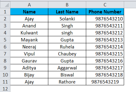
Let us take the example of a phone book sample. It has ten contacts in it with their cell numbers and names. Cell Numbers are in general numeric format; however, the names are in First Name & Last Name Format, which are being separated with space.
Below is a snapshot of the data,
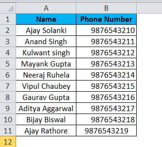
I want to separate the first name and last name to see how many people are there in the phonebook with the name of Ajay.
Let us follow the below steps.
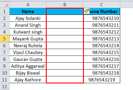
- As we want to split the data in column A into two parts, Insert a column between columns A & B to place the second portion of the text. To insert another column, select column B and right-click on it, and then click insert, or we can use the shortcut key ( Ctrl with +)
(Tip: If we do not insert another column, then the other portion of data will overwrite our data in column B)
- Name the new cell B as the Last Name. Select column A as it needs to be separated, and Go to Data Tab and click on the text to column.
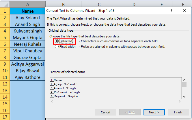
- A dialog box appears which has two options:
Delimited and Fixed width. In the current example, we will use delimited as the number of characters between the first name and last name is not the same in all the cells.
- In a delimited section, click on next, and we can see that we have delimiters means the characters by which the text is separated. In the current scenario, it is a space, so click on space.

(Tip: We have a little box where we can see how the delimiters will affect our current data or, in other terms, how our output will look like).
- Click on Next, and another dialog box appears, which allows us to select the format of data we want.
- Again, in the above step, our data is text, and we do not want to change the format so we can click on finish.
(Tip: In this example, we could simply click on finish to see the output)
Below is the result,
Text to Columns in Excel Example #2
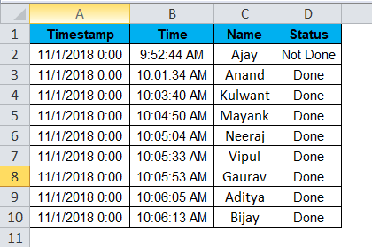
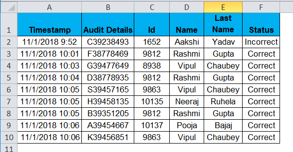
I have asked my students to fill out a google form to submit their responses to whether they have finished their homework. Below is the data,
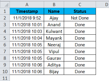
The data in Column A is a timestamp that google form automatically records at the time of data is filled. It contains the date & time of the action done. I want to separate the data and time into separate columns.
- Insert a column between Column A & Column B.
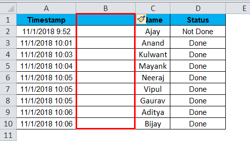
- Select Column A and Go to text to Column under Data Tab and click it.
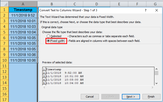
- For the current example, the data in column A has recorded time too, which means the data can be divided into AM & PM too. So we will use a feature called “Fixed Width” in Text to columns.
- Click on Next, and another dialog box appears; it allows us to set field width as how we want to separate the data in this dialogue box. Either we can divide it into two columns, i.e. Date in Date Format and time in AM PM format, or we can have a date in one column, time in another, and AM-PM in another one.
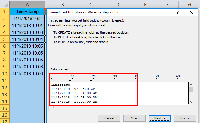
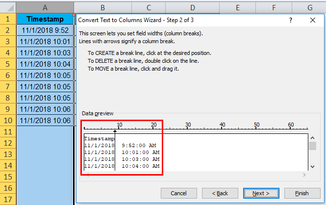
- In the dialog box, we will see the procedures of how to create a line, break a line, and move a line. In this example, I want to split the data into two columns, not in three, as the preview shows above. So I need to delete the line between the second and third columns. To do so, we double-click on the second line.
- When we click on next, the dialog box appears, which allows us to change the format of both columns.
- I want the data in the same format so we can click finish to see the result.
Text to Columns in Excel Example #3
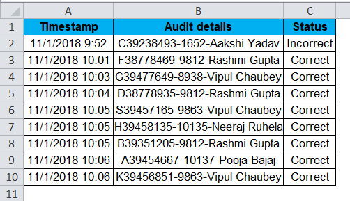
I have the following data with me where in Column B, three texts are separated together with a hyphen (-). I want all three texts in a separate column.
Below is the data,
Let us follow the same procedure, but this time there are three texts, so we will insert two columns instead of one.
- Select Column C and insert three columns.
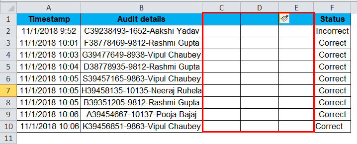
- Select Column B, then go to the text to Column under Data Tab and click it.
- In the current example, a character separates the data, so we will use a delimited feature again.
- As our data is neither separated by Tab, Semi-Colon, or a comma, but it’s a Hyphen (-) and Space. So we will select other and in the other box put “-“in it.
- Click on Finish; as we can see in the preview, this is the result we want to skip the data format dialog box.
- Below is our desired data,
Explanation of Text to Columns in Excel:
From the above example, it is very much clear that text to column separates text into columns.
It is a very unique feature in excel which separates the text as desired.
Things to Remember
- Always Insert a number of columns equal to the number of data that need to be separated in a cell. For Example, if a cell value is A-B-C, then two data need to be separate so insert two columns.
- Identify the delimiter in the case of the delimited feature. In “John, David”, the comma (,) is a delimiter.
- In fixed-width, move the arrow to the desired width.
Recommended Articles
This has been a guide to Text to Columns in Excel. Here we discuss its uses and how to convert Text to Columns in Excel with excel examples and downloadable excel templates. You may also look at these useful functions in excel –
- Excel Text with Formula
- Formatting Text in Excel
- COLUMNS Formula in Excel
- Excel Separate text
В этой статье Вы найдёте несколько способов, как разбить ячейки или целые столбцы в Excel 2010 и 2013. Приведённые примеры и скриншоты иллюстрируют работу с инструментами «Текст по столбцам» и «Мгновенное заполнение», кроме этого Вы увидите подборку формул для разделения имён, текстовых и числовых значений. Этот урок поможет Вам выбрать наилучший метод разбиения данных в Excel.
Говоря в общем, необходимость разбить ячейки в Excel может возникнуть в двух случаях: Во-первых, при импорте информации из какой-либо внешней базы данных или с веб-страницы. При таком импорте все записи копируются в один столбец, а нужно, чтобы они были помещены в разных столбцах. Во-вторых, при разбиении уже существующей таблицы, чтобы получить возможность качественнее настроить работу фильтра, сортировку или для более детального анализа.
- Разбиваем ячейки при помощи инструмента «Текст по столбцам»
- Как разбить объединённые ячейки в Excel
- Разделяем данные в Excel 2013 при помощи инструмента «Мгновенное заполнение»
- Формулы для разбиения столбцов (имен и других текстовых данных)
Содержание
- Разбиваем ячейки в Excel при помощи инструмента «Текст по столбцам»
- Разбиваем текстовые данные с разделителями по столбцам в Excel
- Разбиваем текст фиксированной ширины по нескольким столбцам
- Разбиваем объединённые ячейки в Excel
- Разделяем данные на несколько столбцов в Excel 2013 при помощи мгновенного заполнения
- Как в Excel разбивать ячейки при помощи формул
- Пример 1
- Пример 2
- Пример 3
- Пример 4
- Пример 5
Разбиваем ячейки в Excel при помощи инструмента «Текст по столбцам»
Инструмент «Текст по столбцам» действительно очень удобен, когда нужно разделить данные из одного столбца по нескольким в Excel 2013, 2010, 2007 или 2003.
«Текст по столбцам» позволяет разбивать значения ячеек, отделённые разделителями, или выделять данные фиксированной ширины (когда все значения содержат определённое количество символов). Давайте рассмотрим эти варианты подробнее:
- Как разбить текст с разделителями по столбцам
- Как выделить текстовые данные фиксированной величины
Разбиваем текстовые данные с разделителями по столбцам в Excel
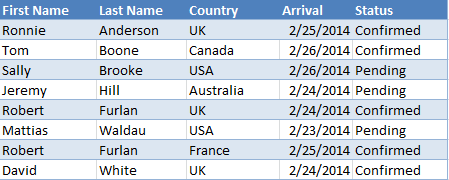
Предположим, есть список участников, приглашённых на конференцию или какое-то другое мероприятие. На рисунке ниже видно, что в столбце Participant (Участник) перечислены имена участников, государство и ожидаемая дата прибытия:
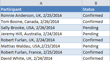
Необходимо разбить этот текст на отдельные столбцы, чтобы таблица имела следующие данные (слева направо): First Name (Имя), Last Name (Фамилия), Country (Страна), Arrival Date (Ожидаемая дата прибытия) и Status (Статус).
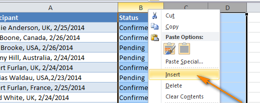
- Если в таблице есть хотя бы один столбец справа от столбца, который необходимо разбить, тогда первым делом создайте новые пустые столбцы, в которые будут помещены полученные данные. Этот шаг необходим для того, чтобы результаты не были записаны поверх уже существующих данных.В нашем примере сразу после столбца Participant находится столбец Status, и мы собираемся добавить между ними новые столбцы Last Name, Country и Arrival Date.Если кто-то забыл, я напомню быстрый способ вставить сразу несколько столбцов на лист Excel. Для этого выберите столбец Status, кликнув по его заголовку, и, удерживая нажатой левую кнопку мыши, протащите указатель вправо, чтобы выделить нужное количество столбцов (сколько хотите вставить). Затем кликните правой кнопкой мыши по выделенной области и в контекстном меню выберите команду Insert (Вставить).

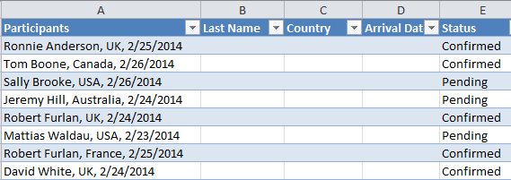
Результат будет примерно таким, что Вы видите на рисунке ниже (новые столбцы вставлены слева от выделенных столбцов):
Примечание: Если у Вас нет столбцов, следующих непосредственно за тем, что Вы хотите разбить, то необходимость в этом шаге отпадает и его можно пропустить. Главное не упустите, что пустых столбцов должно быть не меньше, чем количество столбцов, на которое вы хотите разделить данные.
- Выделите столбец, который требуется разбить. Затем откройте вкладку Data (Данные) > Data Tools (Работа с данными) > Text to Columns (Текст по столбцам).
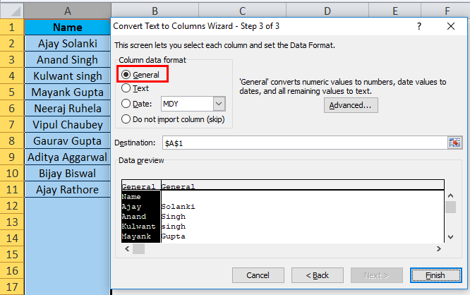
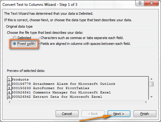
- Откроется диалоговое окно Convert Text to Columns wizard (Мастер распределения текста по столбцам). На первом шаге мастера Вы выбираете формат данных. Так как записи разделены пробелами и запятыми, мы выбираем формат Delimited (С разделителями). Вариант Fixed width (Фиксированной ширины) будет рассмотрен чуть позже. Если все готово, жмите Next (Далее), чтобы продолжить.
- На следующем шаге определяем разделители, которые содержатся в данных, и ограничитель строк.
- Настраиваем разделители. Если данные разделены одним или несколькими разделителями, то нужно выбрать все подходящие варианты в разделе Delimiters (Символом-разделителем является) или ввести свой вариант разделителя в поле Other (Другой).В нашем примере мы выбираем Space (Пробел) и Comma (Запятая), а также ставим галочку напротив параметра Treat consecutive delimiters as one (Считать последовательные разделители одним). Этот параметр поможет избежать лишнего разбиения данных, например, когда между словами есть 2 или более последовательных пробела.
- Настраиваем ограничитель строк. Этот параметр может понадобиться, если в столбце, который Вы разбиваете, содержатся какие-либо значения, заключённые в кавычки или в апострофы, и Вы хотите, чтобы такие участки текста не разбивались, а рассматривались как цельные значения. Например, если Вы выберите в качестве разделителя запятую, а в качестве ограничителя строк – кавычки («), тогда любые слова, заключённые в кавычки (например, «California, USA»), будут помещены в одну ячейку. Если же в качестве ограничителя строк установить значение None (Нет), тогда слово «California» будет помещено в один столбец, а «USA» – в другой.
В нижней части диалогового окна находится область Data preview (Образец разбора данных). Прежде чем нажать Next (Далее) будет разумным пролистать это поле и убедиться, что Excel правильно распределил все данные по столбцам.
- Настраиваем разделители. Если данные разделены одним или несколькими разделителями, то нужно выбрать все подходящие варианты в разделе Delimiters (Символом-разделителем является) или ввести свой вариант разделителя в поле Other (Другой).В нашем примере мы выбираем Space (Пробел) и Comma (Запятая), а также ставим галочку напротив параметра Treat consecutive delimiters as one (Считать последовательные разделители одним). Этот параметр поможет избежать лишнего разбиения данных, например, когда между словами есть 2 или более последовательных пробела.
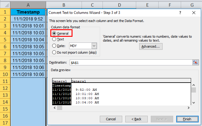
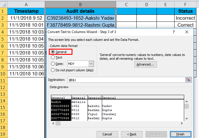
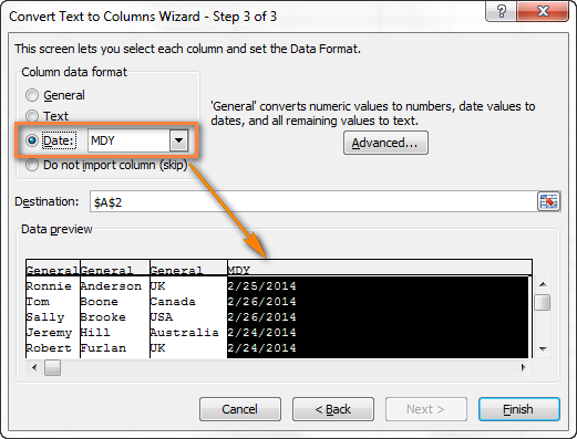
- Осталось сделать всего две вещи – выбрать формат данных и указать, куда поместить разделённые ячейки.В разделе Column data format (Формат данных столбца) Вы можете выбрать формат данных отдельно для каждого столбца, в которые будут помещены разделённые данные. По умолчанию для всех столбцов задан формат General (Общий). Мы оставим его без изменений для первых трёх столбцов, а для четвёртого столбца установим формат Data (Дата), что логично, ведь в этот столбец попадут даты прибытия.Чтобы изменить формат данных для каждого конкретного столбца, выделите его, кликнув по нему в области Data preview (Образец разбора данных), а затем установите желаемый формат в разделе Column data format (Формат данных столбца).
На этом же шаге мастера Вы можете выбрать, в какой столбец поместить разделённые данные. Для этого кликните по иконке выбора диапазона (в терминах Microsoft эта иконка называется Свернуть диалоговое окно) справа от поля Destination (Поместить в) и выберите крайний левый столбец из тех, в которые Вы хотите поместить разделённые данные. К сожалению, невозможно импортировать разделённые данные на другой лист или в другую рабочую книгу, попытка сделать это приведёт к сообщению об ошибке выбора конечной ссылки.
Совет: Если Вы не хотите импортировать какой-то столбец (столбцы), который показан в области Data preview (Образец разбора данных), то выделите его и выберите вариант Do not import column (Пропустить столбец) в разделе Column data format (Формат данных столбца).
- Нажмите Finish (Готово)!
Разбиваем текст фиксированной ширины по нескольким столбцам
Если данные состоят из текстовых или числовых значений с фиксированным количеством символов, Вы можете разбить их на несколько столбцов следующим способом.
К примеру, есть список товаров с ID и наименованием, причем идентификатор товара – это 9 символов, которые стоят перед наименованием этого товара:
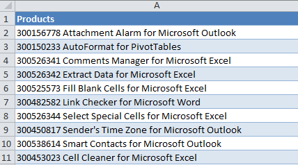
Вот что Вам нужно сделать, чтобы разбить такой столбец на два:
- Запустите инструмент Text to Columns (Текст по столбцам), как мы это делали в предыдущем примере. На первом шаге мастера выберите параметр Fixed width (Фиксированной ширины) и нажмите Next (Далее).
- В разделе Data preview (Образец разбора данных) настройте ширину столбцов. Как видно на рисунке ниже, край столбца символизирует вертикальная линия, и чтобы задать край следующего столбца, просто кликните в нужном месте. Двойной щелчок по вертикальной линии удалит край столбца, а если Вам нужно переместить границу столбца в другое место, просто перетащите вертикальную линию мышью. На самом деле, все эти инструкции подробно расписаны в верхней части диалогового окна 🙂Так как каждый ID товара содержит 9 символов, устанавливаем линию границы столбца на это значение, как показано на рисунке выше.
- На следующем шаге выберите формат данных и укажите ячейки, куда поместить результат, как это было сделано в предыдущем примере, а затем нажмите Finish (Готово).
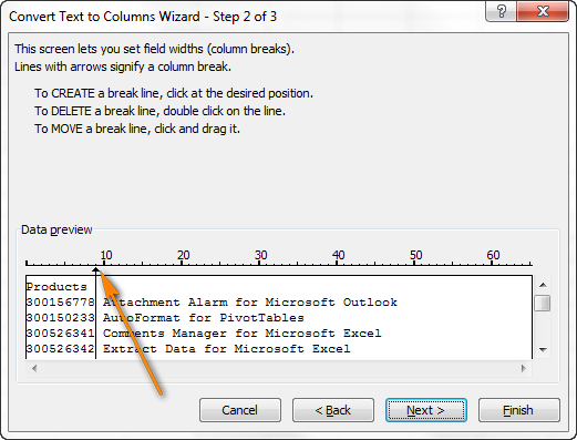 Так как каждый ID товара содержит 9 символов, устанавливаем линию границы столбца на это значение, как показано на рисунке выше.
Разбиваем объединённые ячейки в Excel
Если Вы объединили несколько ячеек на листе Excel и теперь хотите вновь разбить их по отдельным столбцам, откройте вкладку Home (Главная) и в группе команд Alignment (Выравнивание) нажмите маленькую чёрную стрелку рядом с кнопкой Merge & Center (Объединить и поместить в центре). Далее из выпадающего списка выберите Unmerge Cells (Отменить объединение ячеек).

Таким образом объединение ячеек будет отменено, но удовольствие от результата будет испорчено тем, что все данные останутся в левом столбце. Думаю, Вы догадались, что нужно снова использовать функцию Text to Columns (Текст по столбцам), чтобы разбить данные из одного столбца на два или более столбцов.
Разделяем данные на несколько столбцов в Excel 2013 при помощи мгновенного заполнения
Если Вы уже обновились до Excel 2013, то можете воспользоваться преимуществами нового инструмента «Мгновенное заполнение» и заставить Excel автоматически заполнять (в нашем случае – разбивать) данные, при обнаружении определенной закономерности.
Если Вы ещё не знакомы с этой функцией, я попробую кратко объяснить её суть. Этот инструмент анализирует данные, которые Вы вводите на рабочий лист, и пытается выяснить, откуда они взялись и существует ли в них какая-либо закономерность. Как только «Мгновенное заполнение» распознает Ваши действия и вычислит закономерность, Excel предложит вариант, и последовательность записей в новом столбце появится буквально за мгновение.
Таким образом, при помощи этого инструмента Вы можете взять какую-то часть данных, находящихся в одном или нескольких столбцах, и ввести их в новый столбец. Думаю, Вы лучше поймёте о чём я говорю из следующего примера.
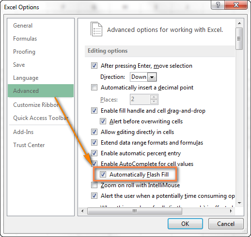
Первым делом, убедитесь, что инструмент «Мгновенное заполнение» включен. Вы найдёте этот параметр на вкладке File (Файл) > Options (Параметры) > Advanced (Дополнительно) > Automatically Flash Fill (Автоматически выполнять мгновенное заполнение).
Теперь давайте посмотрим, как можно автоматически разбить данные по ячейкам. Итак, Вы включили инструмент «Мгновенное заполнение», и начинаете вводить с клавиатуры данные, которые нужно поместить в отдельные ячейки. По мере ввода Excel будет пытаться распознать шаблон в вводимых значениях, и как только он его распознает, данные автоматически будут вставлены в остальные ячейки. Чтобы понять, как это работает, посмотрите на рисунок ниже:
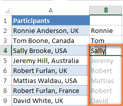
Как видите, я ввёл только пару имён в столбец B, и «Мгновенное заполнение» автоматически заполнило остальные ячейки именами из столбца A. Если вы довольны результатом, просто нажмите Enter, и весь столбец будет заполнен именами. Очень умный инструмент, не правда ли?
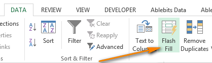
Если «Мгновенное заполнение» включено, но не предлагает никаких вариантов, которые соответствуют определённому шаблону, Вы можете запустить этот инструмент вручную на вкладке Data (Данные) > Flash Fill (Мгновенное заполнение) или нажав сочетание клавиш Ctrl+E.
Как в Excel разбивать ячейки при помощи формул
Существуют формулы, которые могут быть очень полезны, когда возникает необходимость разбить ячейки или столбцы с данными в Excel. На самом деле, следующих шести функций будет достаточно в большинстве случаев – LEFT (ЛЕВСИМВ), MID (ПСТР), RIGHT (ПРАВСИМВ), FIND (НАЙТИ), SEARCH (ПОИСК) и LEN (ДЛСТР). Далее в этом разделе я кратко объясню назначение каждой из этих функций и приведу примеры, которые Вы сможете использовать в своих книгах Excel.
Пример 1
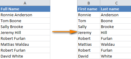
Самая распространённая ситуация, когда могут понадобится эти формулы – это необходимость разделить имена из одного столбца по нескольким. На рисунке ниже показано, какого результата мы пытаемся достичь:
Вы легко сможете разбить такие имена на два столбца при помощи следующих формул:
- Извлекаем имя (столбец First name):
=LEFT(A2,SEARCH(" ",A2,1)-1)
=ЛЕВСИМВ(A2;ПОИСК(" ";A2;1)-1) - Извлекаем фамилию (столбец Last name):
=RIGHT(A2,LEN(A2)-SEARCH(" ",A2,1))
=ПРАВСИМВ(A2;ДЛСТР(A2)-ПОИСК(" ";A2;1))
Для тех, кому интересно, что означают эти формулы, я попробую объяснить более подробно.
SEARCH (ПОИСК) или FIND (НАЙТИ) – это абсолютно идентичные функции, которые выполняют поиск позиции определенной текстовой строки в заданной ячейке. Синтаксис формулы:
=SEARCH(find_text,within_text,[start_num])
=ПОИСК(искомый_текст;текст_для_поиска;[нач_позиция])
В качестве аргументов Вы должны указать: что нужно найти, где нужно искать, а также позицию символа, с которого следует начать поиск. В нашем примере SEARCH(» «,A2,1) или ПОИСК(» «;A2;1) говорит о том, что мы хотим найти символ пробела в ячейке A2 и начнём поиск с первого символа.
Замечание: Если поиск начинается с первого символа, Вы можете вообще пропустить аргумент start_num (нач_позиция) в формуле и упростить её до такого вида:
=LEFT(A2,SEARCH(" ",A2)-1)
=ЛЕВСИМВ(A2;ПОИСК(" ";A2)-1)
LEFT (ЛЕВСИМВ) и RIGHT (ПРАВСИМВ) – возвращает левую или правую часть текста из заданной ячейки соответственно. Синтаксис формулы:
=LEFT(text,[num_chars])
=ЛЕВСИМВ(текст;[количество_знаков])
В качестве аргументов указываем: какой текст взять и сколько символов извлечь. В следующем примере формула будет извлекать левую часть текста из ячейки A2 вплоть до позиции первого найденного пробела.
=LEFT(A2,SEARCH(" ",A2)-1)
=ЛЕВСИМВ(A2;ПОИСК(" ";A2)-1)
LEN (ДЛСТР) – считает длину строки, то есть количество символов в заданной ячейке. Синтаксис формулы:
=LEN(text)
=ДЛСТР(текст)
Следующая формула считает количество символов в ячейке A2:
=LEN(A2)
=ДЛСТР(A2)
Если имена в Вашей таблице содержат отчества или суффиксы, то потребуются немного более сложные формулы с использованием функции MID (ПСТР).
Пример 2
Вот такие формулы нужно использовать, когда имена, которые требуется разбить, содержат отчество или только один инициал отчества посередине.
| A | B | C | D | |
| 1 | Полное имя | Имя | Отчество | Фамилия |
| 2 | Sally K. Brooke | Sally | K. | Brooke |
- Извлекаем имя:
=LEFT(A2,FIND(" ",A2,1)-1)
=ЛЕВСИМВ(A2;НАЙТИ(" ";A2;1)-1) - Извлекаем отчество:
=MID(A2,FIND(" ",A2,1)+1,FIND(" ",A2,FIND(" ",A2,1)+1)-(FIND(" ",A2,1)+1))
=ПСТР(A2;НАЙТИ(" ";A2;1)+1;НАЙТИ(" ";A2;НАЙТИ(" ";A2;1)+1)-(НАЙТИ(" ";A2;1)+1)) - Извлекаем фамилию:
=RIGHT(A2,LEN(A2)- FIND(" ",A2,FIND(" ",A2,1)+1))
=ПРАВСИМВ(A2;ДЛСТР(A2)-НАЙТИ(" ";A2;НАЙТИ(" ";A2;1)+1))
Функция MID (ПСТР) – извлекает часть текстовой строки (то есть заданное количество символов). Синтаксис:
=MID(text,start_num,num_chars)
=ПСТР(текст;начальная_позиция;количество_знаков)
В качестве аргументов функции указываем: какой текст взять, позицию символа, с которого нужно начать, и сколько символов извлечь.
Пример 3
Вы можете использовать аналогичные формулы, чтобы разбить имена с суффиксами в конце:
| A | B | C | D | |
| 1 | Полное имя | Имя | Фамилия | Суффикс |
| 2 | Robert Furlan Jr. | Robert | Furlan | Jr. |
- Извлекаем имя:
=LEFT(A2,FIND(" ",A2,1)-1)
=ЛЕВСИМВ(A2;НАЙТИ(" ";A2;1)-1) - Извлекаем фамилию:
=MID(A2,FIND(" ",A2,1)+1,FIND(" ",A2,FIND(" ",A2,1)+1)-(FIND(" ",A2,1)+1))
=ПСТР(A2;НАЙТИ(" ";A2;1)+1;НАЙТИ(" ";A2;НАЙТИ(" ";A2;1)+1)-(НАЙТИ(" ";A2;1)+1)) - Извлекаем суффикс:
=RIGHT(A2,LEN(A2)-FIND(" ",A2,FIND(" ",A2,1)+1))
=ПРАВСИМВ(A2;ДЛСТР(A2)-НАЙТИ(" ";A2;НАЙТИ(" ";A2;1)+1))
Пример 4
А вот формулы, позволяющие разбить имена с фамилией, стоящей впереди и отделенной от имени запятой, и отчеством, находящимся в конце:
| A | B | C | D | |
| 1 | Полное имя | Имя | Отчество | Фамилия |
| 2 | White, David Mark | David | Mark | White |
- Извлекаем имя:
=MID(A2,SEARCH(" ",A2,1)+1,FIND(" ",A2,FIND(" ",A2,1)+1)-(FIND(" ",A2,1)+1))
=ПСТР(A2;ПОИСК(" ";A2;1)+1;НАЙТИ(" ";A2;НАЙТИ(" ";A2;1)+1)-(НАЙТИ(" ";A2;1)+1)) - Извлекаем отчество:
=RIGHT(A2,LEN(A2)- FIND(" ",A2,FIND(" ",A2,1)+1))
=ПРАВСИМВ(A2;ДЛСТР(A2)-НАЙТИ(" ";A2;НАЙТИ(" ";A2;1)+1)) - Извлекаем фамилию:
=LEFT(A2,FIND(" ",A2,1)-2)
=ЛЕВСИМВ(A2;НАЙТИ(" ";A2;1)-2)
Пример 5
Как Вы понимаете, эти формулы работают не только для разделения имён в Excel. Вы можете использовать их для разбиения любых данных из одного столбца по нескольким. Например, следующие формулы Вы можете использовать, чтобы разбить текстовые данные, разделённые запятыми:
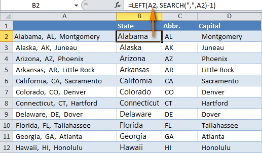
| A | B | C | D | |
| 1 | Полное обозначение | Штат | Аббревиатура | Столица |
| 2 | Alabama, AL, Montgomery | Alabama | AL | Montgomery |
- Извлекаем название штата:
=LEFT(A2,SEARCH(",",A2)-1)
=ЛЕВСИМВ(A2;ПОИСК(",";A2)-1) - Извлекаем аббревиатуру штата:
=MID(A2,SEARCH(",",A2)+2,SEARCH(",",A2,SEARCH(",",A2)+2)-SEARCH(",",A2)-2)
=ПСТР(A2;ПОИСК(",";A2)+2;ПОИСК(",";A2;ПОИСК(",";A2)+2)-ПОИСК(",";A2)-2) - Извлекаем столицу штата:
=RIGHT(A2,LEN(A2)-(SEARCH(",",A2,SEARCH(",",A2)+1)+1))
=ПРАВСИМВ(A2;ДЛСТР(A2)-(ПОИСК(",";A2;ПОИСК(",";A2)+1)+1))
А вот пример реальных данных из Excel 2010. Данные из первого столбца разбиты на три отдельных столбца:
Оцените качество статьи. Нам важно ваше мнение: