
Microsoft Excel 2013 is such a versatile program that it can effectively be used for a number of purposes. So while one user might not consider changing something like the direction in which a worksheet is oriented, a different user might find that to be something that would be beneficial.
If you fall into that second group of Excel users and would like to change your Excel spreadsheet so that the column lettering starts at the right side of the sheet, then our guide below will show you where to find and change that setting.
How to Change the Spreadsheet Direction in Excel 2013
The steps below will change the default settings in Excel 2013 so that the spreadsheet is configured from right to left, instead of from left to right. This will put the “A” column at the right side of the spreadsheet, which is also where your cursor will start. These changes only apply to new workbooks that you create in Excel after making this change. Previous workbooks will be unaffected.
Step 1: Open Excel 2013.
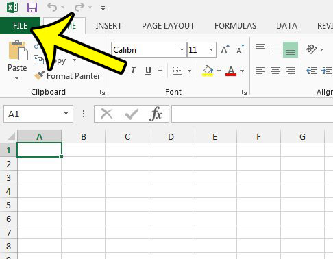
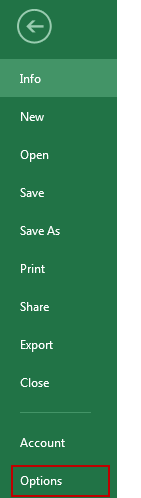
Step 2: Click the File tab at the top-left corner of the window.
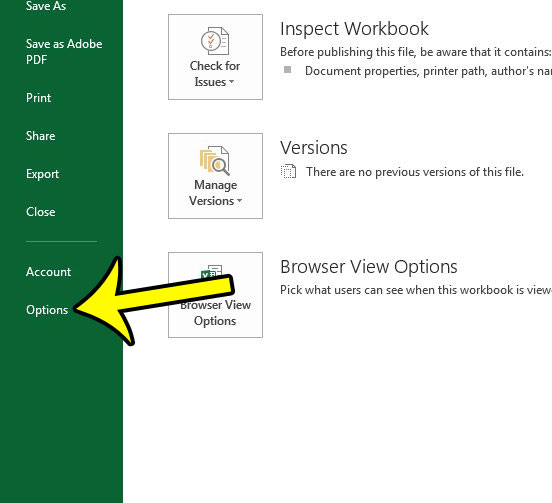
Step 2: Click Options in the left column.
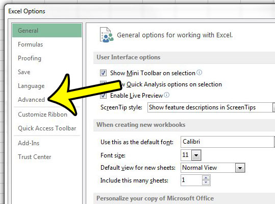
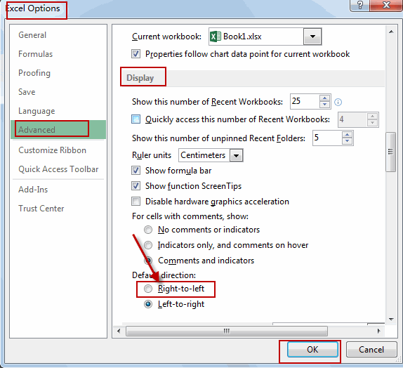
Step 3: Click the Advanced tab at the left side of the Excel Options window.
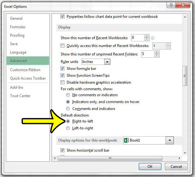
Step 4: Scroll down to the Display section, then click the circle to the left of Right-to-left under Default direction. You can then click the OK button at the bottom of the window.
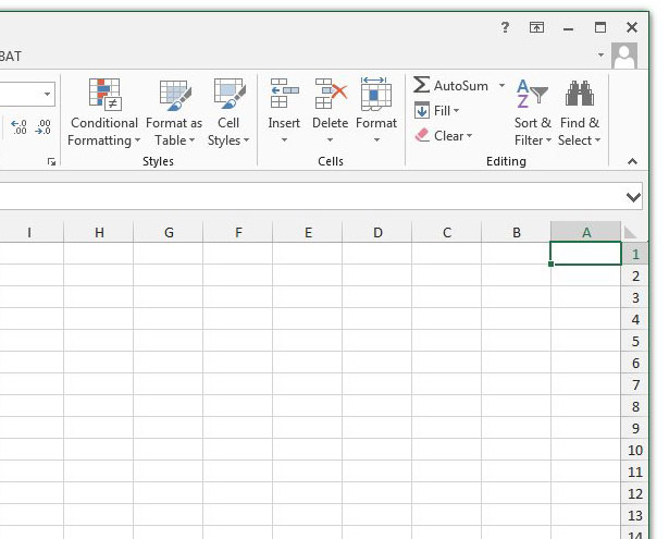
Now when you re-open Excel 2013, then default direction for the spreadsheet should be right to left. It should look something like the picture below –
If changing this setting does not result in a spreadsheet that goes from right to left, then you might be using a user template that is preventing this change from occurring. You can find and delete Excel user templates in this folder – C:UsersYourUserNameAppDataRoamingMicrosoftExcelXLSTART
Note that deleting a user template may result in significant changes to your Excel experience if you have made a lot of customizations to that template. If you are unsure about whether or not you should delete a template, consult your system administrator.
If you often print your spreadsheets, then read this article about printing a document title at the top of every page. It’s a helpful thing to add to your spreadsheets that makes them easier to identify later on.

Kermit Matthews is a freelance writer based in Philadelphia, Pennsylvania with more than a decade of experience writing technology guides. He has a Bachelor’s and Master’s degree in Computer Science and has spent much of his professional career in IT management.
He specializes in writing content about iPhones, Android devices, Microsoft Office, and many other popular applications and devices.
Read his full bio here.
If you want to change the default Excel worksheet direction, you need to go through this article to learn the steps. There are three ways to change the default direction of an Excel worksheet – using in-built Settings, Local Group Policy Editor, and Registry Editor. This article comes with all three methods, and you can follow any one of them.
If you open an Excel worksheet, you can find some rows and columns, which represent Excel. If you observe more, you can find A, B, C, D from left to right, which is the typical formation. However, if you want to change it and show the sheet from right to left instead of left to right due to any reason, here is how you can do that.

To change the default Excel worksheet direction, follow these steps:
- Open an Excel worksheet on your PC.
- Click on File and select Options.
- Switch to the Advanced tab.
- Find the Display section.
- Choose Right-to-left option.
- Click the OK button.
To learn more about these steps, continue reading.
First, you need to open an Excel worksheet on your PC and click on the File menu visible on the top-left corner. Then, select the Options to open the Excel Options panel.
After that, switch to the Advanced tab and find out the Display section. Here you can find an option called Default direction. From here, you need to choose the Right-to-left option.
Click the OK button to save the change. Next, you need to open a new worksheet to find the change.
As mentioned earlier, you can do the same thing using the Local Group Policy Editor and the Registry Editor. If you want to follow the GPEDIT method, you must download the administrative templates for Office.
How to change default Excel worksheet direction using Group Policy
To change default Excel worksheet direction using Group Policy, follow these steps:
- Press Win+R to display the Run dialog.
- Type gpedit.msc and press the Enter button.
- Go to Advanced in User Configuration.
- Double-click on the Default sheet direction.
- Choose the Enabled option.
- Select the Right-to-left option.
- Click the OK button.
Let’s check out these steps in detail.
To get started, you need to open the Local Group Policy Editor on your computer. For that, press Win+R, type gpedit.msc, and press the Enter button.
Next, navigate to the following path:
User Configuration > Administrative Templates > Microsoft Excel 2016 > Excel Options > Advanced
In the Advanced folder, you can see a setting called Default sheet direction. You need to double-click on it and select the Enabled option.
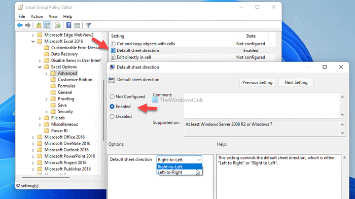
Following that, expand the drop-down menu and select the Right-to-left option.
Click the OK button to save the change. Once done, you need to restart Excel to find the change.
How to change default Excel worksheet direction using Registry
To change default Excel worksheet direction using Registry, follow these steps:
- Search for registry in the Taskbar search box.
- Click on the individual search result.
- Click the Yes button.
- Navigate to office in HKCU.
- Right-click on empty space > New > Key.
- Name it as 0.
- Repeat this step to create a sub-key named excel.
- Right-click on excel > New > Keyand name it as options.
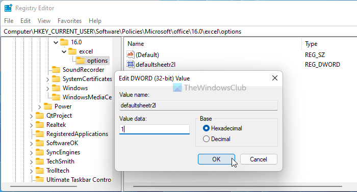
- Right-click on options > New > DWORD (32-bit) Value.
- Set the name as defaultsheetr2l.
- Double-click on it to set the Value data as 1.
- Click the OK button and restart your computer.
Let’s learn more about these steps in detail.
First, search for registry or registry editor in the Taskbar search box, click the individual search result, and click on the OK button to open Registry Editor. Then, navigate to the following path:
HKEY_CURRENT_USERSoftwarePoliciesMicrosoftoffice
Select the office key, right-click on empty space, select New > Key, and name it as 16.0.
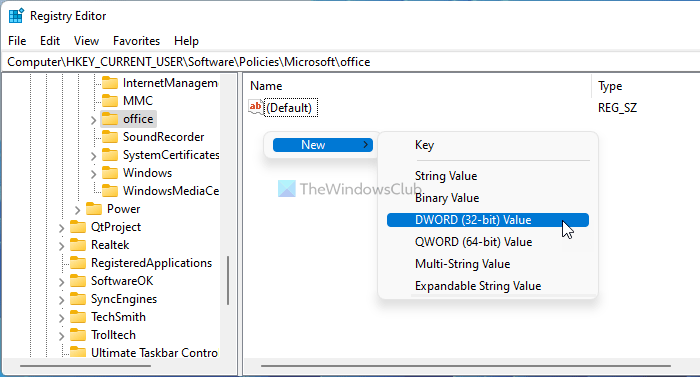
Then, repeat the same step to create a sub-key named excel. Following that, do the same under the excel key to create another sub-key called options.
Once the options key is made, you need to create a REG_DWORD value. For that, right-click on options > New > Key and set the name as defaultsheetr2l.
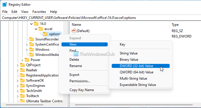
Double-click on it to set the Value data as 1.
Click the OK button and restart your computer to get the change.
Read: How to open two Excel files in separate windows.
How to show Sheet from right to left in Excel?
To show sheets from right to left in Excel, you need to follow the above-mentioned guides. You can open the Excel Options panel and switch to the Advanced tab. Then, find the Display section, and find the Default direction menu. Choose the Right-to-left option and click the OK button to save the change.
How to change display direction in Excel?
To change the display direction in Excel, you can use the in-built settings, GPEDIT and REGEDIT. In the Group Policy, navigate to Microsoft Excel 2016 > Excel Options > Advanced in User Configuration. Then, double-click on the Default sheet direction setting and choose the Enabled option. After that, select the Right-to-left option and click the OK button.
That’s all! Hope this guide was handy.
This post will guide you how to change worksheet direction from default to right-to-left in your worksheet in Excel 2013/2016. How do I change worksheet direction in Excel.
Change Worksheet Direction
By default, the worksheet direction is from left to right. And if you want to change the direction from right to left in your current worksheet. How to do it. You can do the following steps:
#1 click File tab, and select Options from the left menu list. And the Excel Options dialog will open.
#2 click Advanced menu in the Excel Options dialog, and scroll down to Display section, and check Right-to-left radio button under Default direction section.
#3 click Ok button. Click “Add” button on the sheet tab to create a new worksheet. You would notice that the current worksheet direction has been changed to right-to-left.
Note: This method is only valid for the newly worksheet.
Why to create standard charts in Excel? Try something extraordinary. Let’s teach yourself how to create a chart from right to left. It means that that axis will flip on the right side of your chart. Just follow these steps.
Chart from Right to Left
1. Enter data into Excel sheet and select the data.

2. Go to insert and select any of the desired chart.

3. Right-click the vertical axis, then click format axis and go labels.

4. Now open the drop-down menu under labels and select high to move the vertical axis towards the left. Ready chart from right to left looks like that:

Here you can download a free Chart from right to left template.
Values in Reverse Order
You can also set values in reverse order. Just right click your axis and choose Format Axis.

From the menu choose Values in Reverse order.

Now your bar chart is inserted from right to left.

This is how to flip a chart in Excel.
How to move X axis
If you are not satisfied with rotating your chart, then move the axis as well.
In Excel, you can move the axis so that it intersects the graph at the point that suits you.
Now I will teach you how to move the x axis higher. I don’t want the x axis to be at the bottom of the plot. I will move the x axis higher in the chart.
I don’t want the x axis to cross the y axis at point 0. I want the x axis to intersect the y axis at 0.2.
It’s easy to move the x-axis up the chart. To change the position of the x-axis, left-click on it. In the Formax Axis menu, go to Axis Options. In the Vertical axis crosses field, click on Axis value and enter the value. I entered 0.2.

The x axis has moved and now intersects the y axis at 0.2.

I hope you enjoyed the trick.
This demonstration covers how to use the LEFT and Right Functions in Excel. These are text functions. In the LEFT function, you can pull a set number of characters out of a cell into another cell starting at the leftmost point. The RIGHT function performs the same except starting at the rightmost point.
Both functions are related to the MID function, which we covered back in September. At the time, one of our customers asked for a demo on the MID function. Since then, we’ve had several follow up requests on the LEFT and RIGHT.
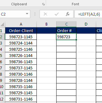
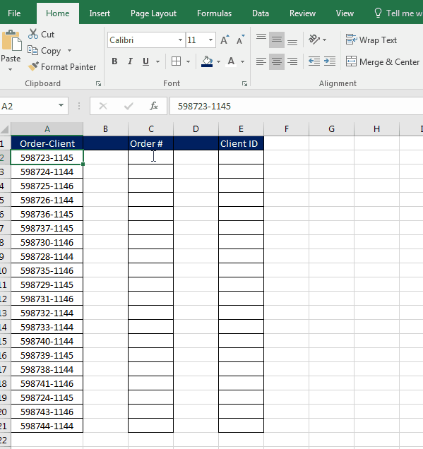
For today’s demonstration, we will be using the following spreadsheet:
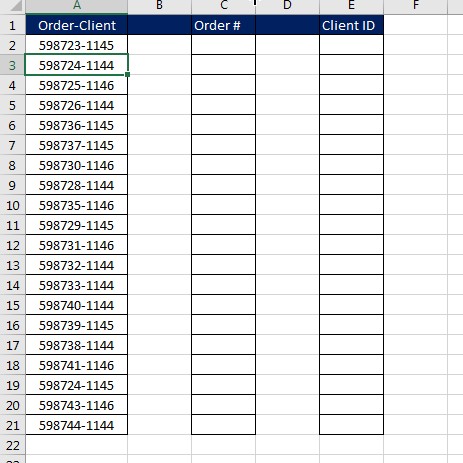
In this example, Column A contains a 6-digit number hyphenated with a 4-digit number. The 6-digit number is the order number and the 4 digit is the client ID. Your job is to separate the order number and client ID into Columns C and E, respectively.
How is this done?
For the order number, we will use the LEFT function. We know the code is 6 digits, so we have the number of characters. So in cell C2, you will enter the following formula:
=LEFT(A2,6)
For the client ID, we will use the RIGHT function. In cell E2, you will enter the following formula:
=RIGHT(A2,4)
LEFT Function Syntax:
=LEFT(Destination Cell, Number of Characters)
This tells Excel: Starting on the left of this specified cell, copy to this many characters.
RIGHT Function Syntax:
=RIGHT(Destination Cell, Number of Characters)
This tells Excel: Starting on the right of the specified cell, copy to this many characters.
As you can see in the above demonstration, once the functions have been entered, they can be copied all the way down to finish filling in the data.
We at Learn Excel Now hope you feel comfortable using the RIGHT and LEFT functions.
Like Learn Excel Now? Follow us on social media and share our content with your networks! And don’t forget to sign up for the Newsletter.
Kevin – Learn Excel Now