
Excel for Microsoft 365 Excel 2021 Excel 2019 Excel 2016 Excel 2013 Excel 2010 More…Less
Excel doesn’t have a default function that displays numbers as English words in a worksheet, but you can add this capability by pasting the following SpellNumber function code into a VBA (Visual Basic for Applications) module. This function lets you convert dollar and cent amounts to words with a formula, so 22.50 would read as Twenty-Two Dollars and Fifty Cents. This can be very useful if you’re using Excel as a template to print checks.
If you want to convert numeric values to text format without displaying them as words, use the TEXT function instead.
Note: Microsoft provides programming examples for illustration only, without warranty either expressed or implied. This includes, but is not limited to, the implied warranties of merchantability or fitness for a particular purpose. This article assumes that you are familiar with the VBA programming language, and with the tools that are used to create and to debug procedures. Microsoft support engineers can help explain the functionality of a particular procedure. However, they will not modify these examples to provide added functionality, or construct procedures to meet your specific requirements.
Create the SpellNumber function to convert numbers to words
-
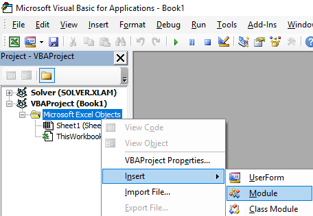
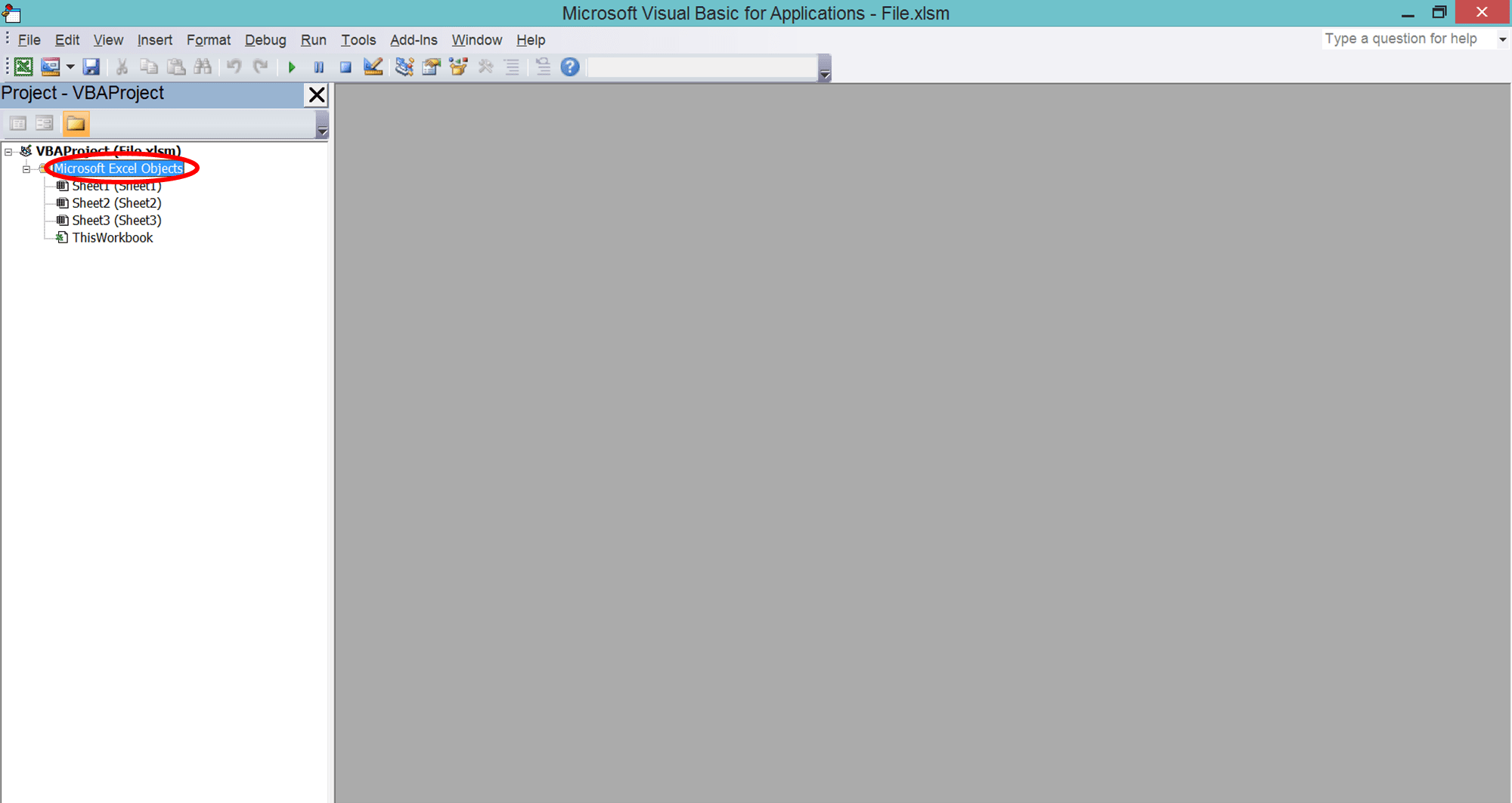
Use the keyboard shortcut, Alt + F11 to open the Visual Basic Editor (VBE).
-
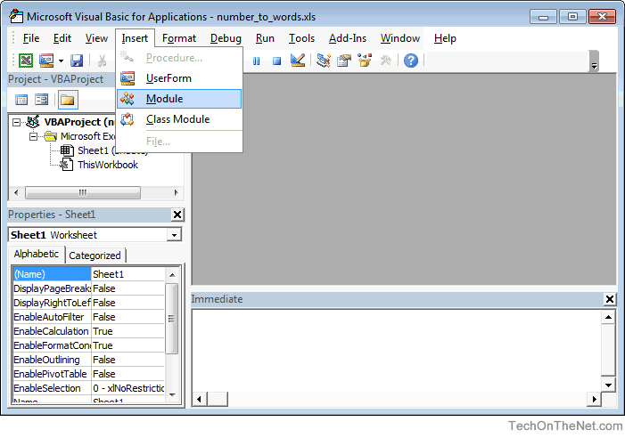
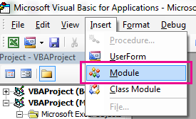
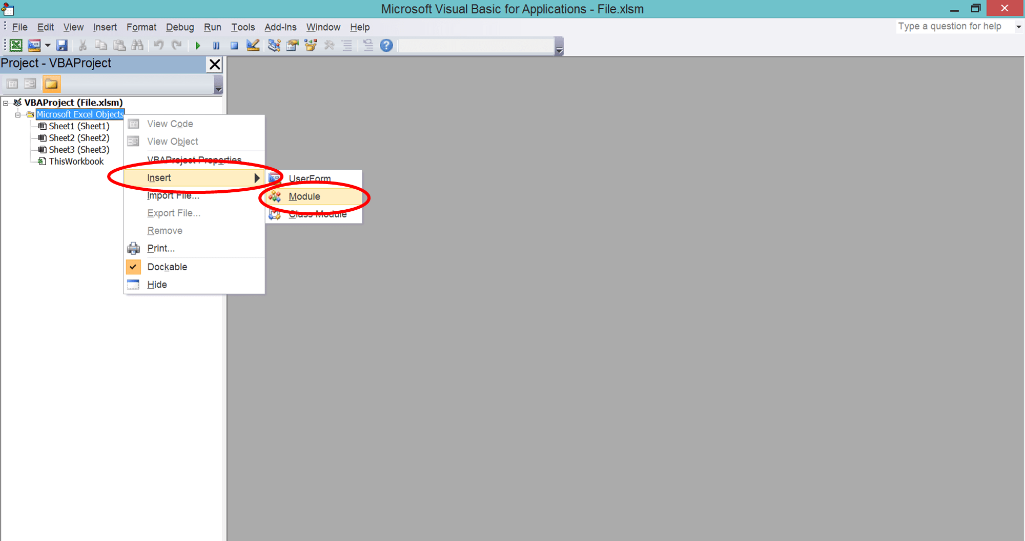
Click the Insert tab, and click Module.

-
Copy the following lines of code.
Note: Known as a User Defined Function (UDF), this code automates the task of converting numbers to text throughout your worksheet.
Option Explicit 'Main Function Function SpellNumber(ByVal MyNumber) Dim Dollars, Cents, Temp Dim DecimalPlace, Count ReDim Place(9) As String Place(2) = " Thousand " Place(3) = " Million " Place(4) = " Billion " Place(5) = " Trillion " ' String representation of amount. MyNumber = Trim(Str(MyNumber)) ' Position of decimal place 0 if none. DecimalPlace = InStr(MyNumber, ".") ' Convert cents and set MyNumber to dollar amount. If DecimalPlace > 0 Then Cents = GetTens(Left(Mid(MyNumber, DecimalPlace + 1) & _ "00", 2)) MyNumber = Trim(Left(MyNumber, DecimalPlace - 1)) End If Count = 1 Do While MyNumber <> "" Temp = GetHundreds(Right(MyNumber, 3)) If Temp <> "" Then Dollars = Temp & Place(Count) & Dollars If Len(MyNumber) > 3 Then MyNumber = Left(MyNumber, Len(MyNumber) - 3) Else MyNumber = "" End If Count = Count + 1 Loop Select Case Dollars Case "" Dollars = "No Dollars" Case "One" Dollars = "One Dollar" Case Else Dollars = Dollars & " Dollars" End Select Select Case Cents Case "" Cents = " and No Cents" Case "One" Cents = " and One Cent" Case Else Cents = " and " & Cents & " Cents" End Select SpellNumber = Dollars & Cents End Function ' Converts a number from 100-999 into text Function GetHundreds(ByVal MyNumber) Dim Result As String If Val(MyNumber) = 0 Then Exit Function MyNumber = Right("000" & MyNumber, 3) ' Convert the hundreds place. If Mid(MyNumber, 1, 1) <> "0" Then Result = GetDigit(Mid(MyNumber, 1, 1)) & " Hundred " End If ' Convert the tens and ones place. If Mid(MyNumber, 2, 1) <> "0" Then Result = Result & GetTens(Mid(MyNumber, 2)) Else Result = Result & GetDigit(Mid(MyNumber, 3)) End If GetHundreds = Result End Function ' Converts a number from 10 to 99 into text. Function GetTens(TensText) Dim Result As String Result = "" ' Null out the temporary function value. If Val(Left(TensText, 1)) = 1 Then ' If value between 10-19... Select Case Val(TensText) Case 10: Result = "Ten" Case 11: Result = "Eleven" Case 12: Result = "Twelve" Case 13: Result = "Thirteen" Case 14: Result = "Fourteen" Case 15: Result = "Fifteen" Case 16: Result = "Sixteen" Case 17: Result = "Seventeen" Case 18: Result = "Eighteen" Case 19: Result = "Nineteen" Case Else End Select Else ' If value between 20-99... Select Case Val(Left(TensText, 1)) Case 2: Result = "Twenty " Case 3: Result = "Thirty " Case 4: Result = "Forty " Case 5: Result = "Fifty " Case 6: Result = "Sixty " Case 7: Result = "Seventy " Case 8: Result = "Eighty " Case 9: Result = "Ninety " Case Else End Select Result = Result & GetDigit _ (Right(TensText, 1)) ' Retrieve ones place. End If GetTens = Result End Function ' Converts a number from 1 to 9 into text. Function GetDigit(Digit) Select Case Val(Digit) Case 1: GetDigit = "One" Case 2: GetDigit = "Two" Case 3: GetDigit = "Three" Case 4: GetDigit = "Four" Case 5: GetDigit = "Five" Case 6: GetDigit = "Six" Case 7: GetDigit = "Seven" Case 8: GetDigit = "Eight" Case 9: GetDigit = "Nine" Case Else: GetDigit = "" End Select End Function -
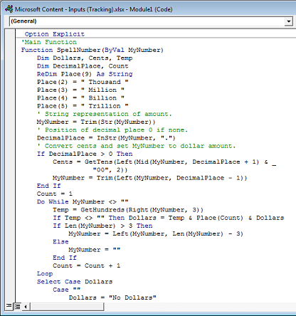
Paste the lines of code into the Module1 (Code) box.
-
Press Alt + Q to return to Excel. The SpellNumber function is now ready to use.
Note: This function works only for the current workbook. To use this function in another workbook, you must repeat the steps to copy and paste the code in that workbook.
Top of Page
Use the SpellNumber function in individual cells
-
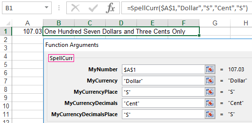
Type the formula =SpellNumber(A1) into the cell where you want to display a written number, where A1 is the cell containing the number you want to convert. You can also manually type the value like =SpellNumber(22.50).
-
Press Enter to confirm the formula.
Top of Page
Save your SpellNumber function workbook
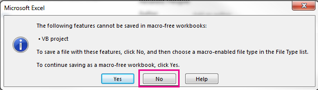
Excel cannot save a workbook with macro functions in the standard macro-free workbook format (.xlsx). If you click File > Save. A VB project dialog box opens. Click No.
You can save your file as an Excel Macro-Enabled Workbook (.xlsm) to keep your file in its current format.
-
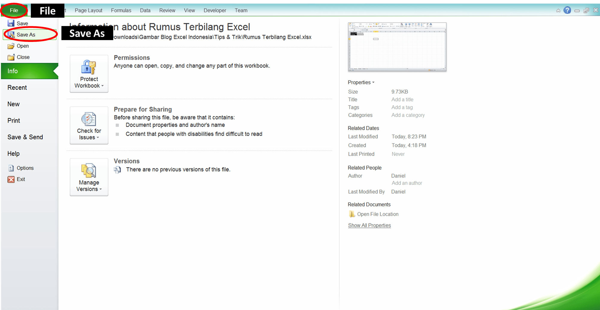
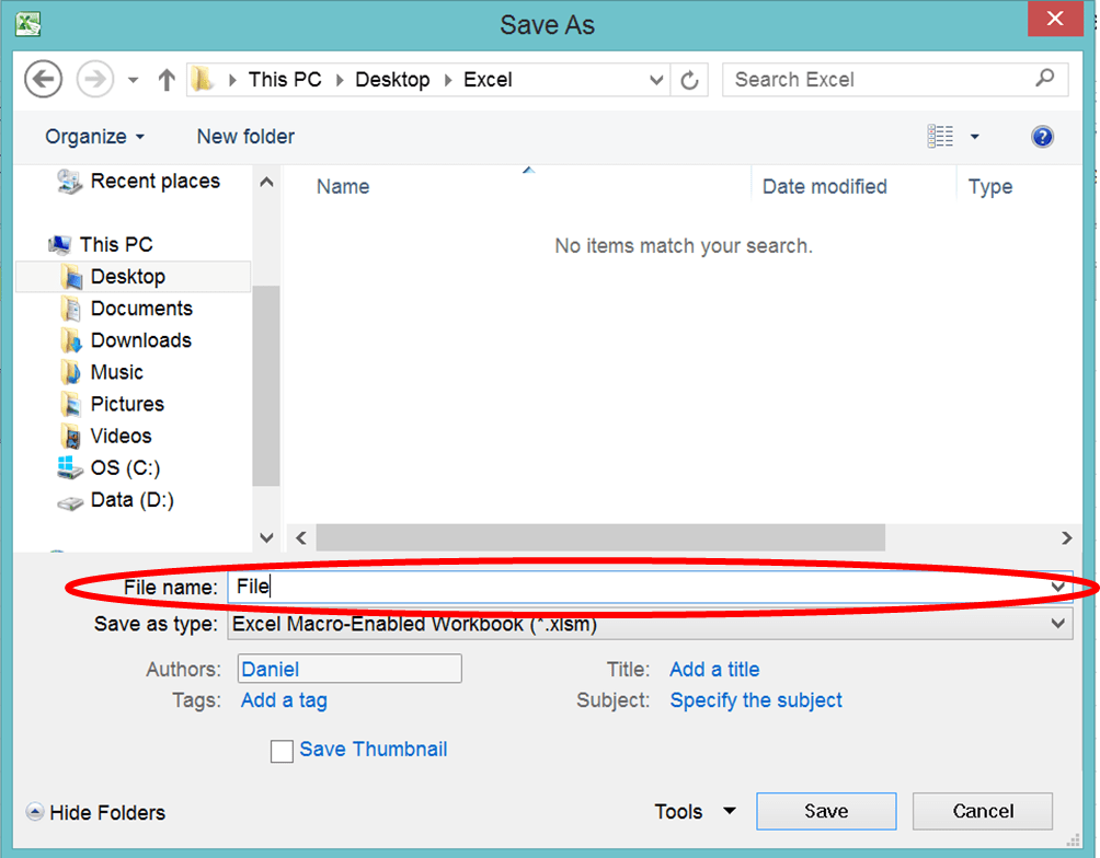
Click File > Save As.
-
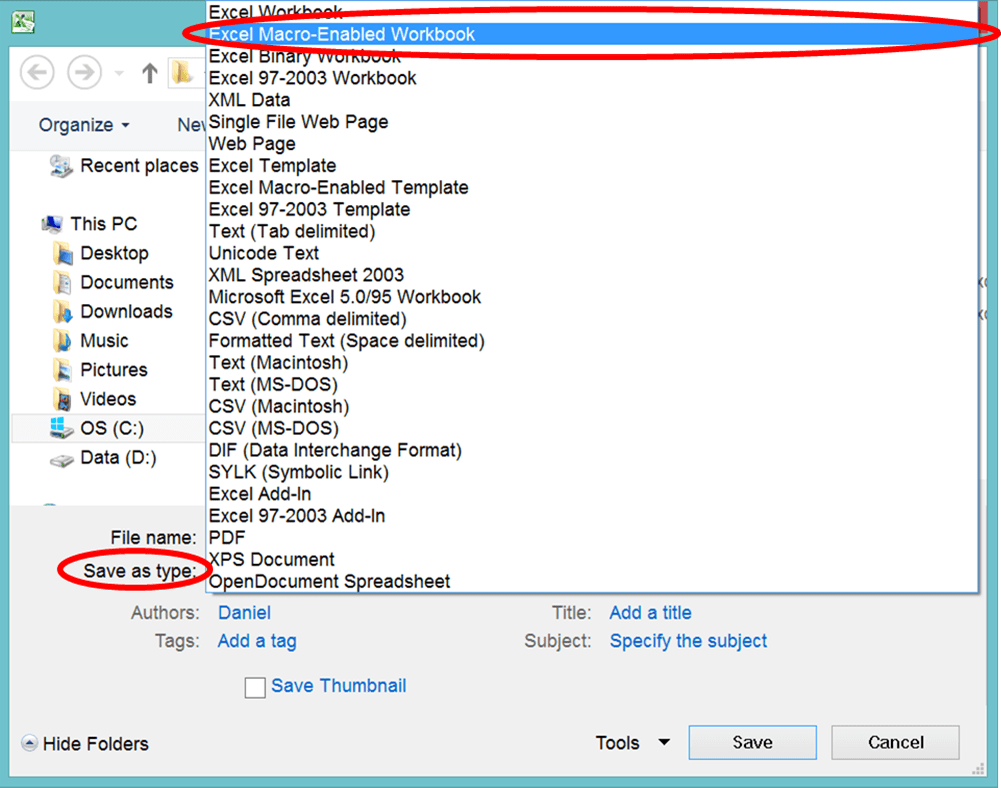
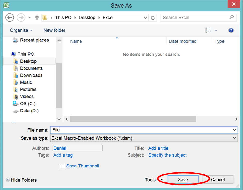
Click the Save as type drop-down menu, and select Excel Macro-Enabled Workbook.
-
Click Save.
Top of Page
See Also
TEXT function
Need more help?
Want more options?
Explore subscription benefits, browse training courses, learn how to secure your device, and more.
Communities help you ask and answer questions, give feedback, and hear from experts with rich knowledge.

This Excel tutorial explains how to convert number into words (with screenshots and step-by-step instructions).
Question: In Microsoft Excel, how can I convert a numeric value to words? For example, for a value of 1, could the cell show the word «one» instead?
Answer: There is no-built in Excel function that will convert a number into words. Instead, you need to create a custom function to convert the number into words yourself. Let’s explore how.
To see the completed function and how it is used in the example below, download the example spreadsheet.
Download Example
TIP: When you create a custom function in Excel, it will create macro code. When you open your file after creating the custom function, it will warn that there are macros in the spreadsheet. You will need to enable the macros for the function to work properly.
Let’s get started. First, you’ll need to open your Excel spreadsheet and press Alt+F11 to open the Microsoft Visual Basic for Applications window. Under the Insert menu, select Module.
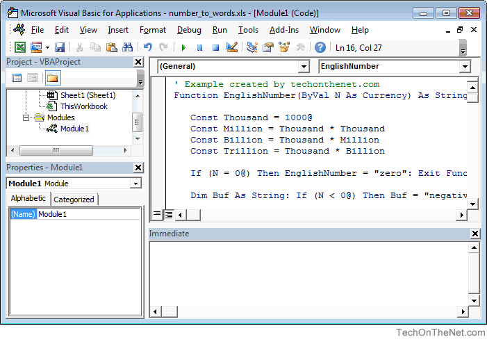
This will insert a new module in your spreadsheet called Module1. Paste the following two functions into the new module.
' Example created by techonthenet.com
Function EnglishNumber(ByVal N As Currency) As String

   Const Thousand = 1000@
   Const Million = Thousand * Thousand
   Const Billion = Thousand * Million
   Const Trillion = Thousand * Billion

   If (N = 0@) Then EnglishNumber = "zero": Exit Function

   Dim Buf As String: If (N < 0@) Then Buf = "negative " Else Buf = ""
   Dim Frac As Currency: Frac = Abs(N - Fix(N))
   If (N < 0@ Or Frac <> 0@) Then N = Abs(Fix(N))
   Dim AtLeastOne As Integer: AtLeastOne = N >= 1

   If (N >= Trillion) Then
      Buf = Buf & EnglishNumberDigitGroup(Int(N / Trillion)) & " trillion"
      N = N - Int(N / Trillion) * Trillion
      If (N >= 1@) Then Buf = Buf & " "
   End If

   If (N >= Billion) Then
      Buf = Buf & EnglishNumberDigitGroup(Int(N / Billion)) & " billion"
      N = N - Int(N / Billion) * Billion
      If (N >= 1@) Then Buf = Buf & " "
   End If

   If (N >= Million) Then
      Buf = Buf & EnglishNumberDigitGroup(N  Million) & " million"
      N = N Mod Million
      If (N >= 1@) Then Buf = Buf & " "
   End If

   If (N >= Thousand) Then
      Buf = Buf & EnglishNumberDigitGroup(N  Thousand) & " thousand"
      N = N Mod Thousand
      If (N >= 1@) Then Buf = Buf & " "
   End If

   If (N >= 1@) Then
      Buf = Buf & EnglishNumberDigitGroup(N)
   End If

   EnglishNumber = Buf
End Function

Private Function EnglishNumberDigitGroup(ByVal N As Integer) As String

   Const Hundred = " hundred"
   Const One = "one"
   Const Two = "two"
   Const Three = "three"
   Const Four = "four"
   Const Five = "five"
   Const Six = "six"
   Const Seven = "seven"
   Const Eight = "eight"
   Const Nine = "nine"
   Dim Buf As String: Buf = ""
   Dim Flag As Integer: Flag = False

   Select Case (N  100)
      Case 0: Buf = "": Flag = False
      Case 1: Buf = One & Hundred: Flag = True
      Case 2: Buf = Two & Hundred: Flag = True
      Case 3: Buf = Three & Hundred: Flag = True
      Case 4: Buf = Four & Hundred: Flag = True
      Case 5: Buf = Five & Hundred: Flag = True
      Case 6: Buf = Six & Hundred: Flag = True
      Case 7: Buf = Seven & Hundred: Flag = True
      Case 8: Buf = Eight & Hundred: Flag = True
      Case 9: Buf = Nine & Hundred: Flag = True
   End Select

   If (Flag <> False) Then N = N Mod 100
   If (N > 0) Then
      If (Flag <> False) Then Buf = Buf & " "
   Else
      EnglishNumberDigitGroup = Buf
      Exit Function
   End If

   Select Case (N  10)
      Case 0, 1: Flag = False
      Case 2: Buf = Buf & "twenty": Flag = True
      Case 3: Buf = Buf & "thirty": Flag = True
      Case 4: Buf = Buf & "forty": Flag = True
      Case 5: Buf = Buf & "fifty": Flag = True
      Case 6: Buf = Buf & "sixty": Flag = True
      Case 7: Buf = Buf & "seventy": Flag = True
      Case 8: Buf = Buf & "eighty": Flag = True
      Case 9: Buf = Buf & "ninety": Flag = True
   End Select

   If (Flag <> False) Then N = N Mod 10
   If (N > 0) Then
      If (Flag <> False) Then Buf = Buf & "-"
   Else
      EnglishNumberDigitGroup = Buf
      Exit Function
   End If

   Select Case (N)
      Case 0:
      Case 1: Buf = Buf & One
      Case 2: Buf = Buf & Two
      Case 3: Buf = Buf & Three
      Case 4: Buf = Buf & Four
      Case 5: Buf = Buf & Five
      Case 6: Buf = Buf & Six
      Case 7: Buf = Buf & Seven
      Case 8: Buf = Buf & Eight
      Case 9: Buf = Buf & Nine
      Case 10: Buf = Buf & "ten"
      Case 11: Buf = Buf & "eleven"
      Case 12: Buf = Buf & "twelve"
      Case 13: Buf = Buf & "thirteen"
      Case 14: Buf = Buf & "fourteen"
      Case 15: Buf = Buf & "fifteen"
      Case 16: Buf = Buf & "sixteen"
      Case 17: Buf = Buf & "seventeen"
      Case 18: Buf = Buf & "eighteen"
      Case 19: Buf = Buf & "nineteen"
   End Select

   EnglishNumberDigitGroup = Buf

End Function
Your Excel window should look as follows:
Click the Save button (disk icon) and then go back to your spreadsheet window.
You can now use the EnglishNumber function to convert a number to words. It will work just like any other worksheet function. Just reference the EnglishNumber function in your Excel spreadsheet as follows:
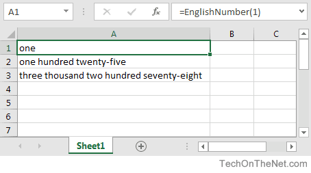
Based on the spreadsheet above, the EnglishNumber function will return the following:
=EnglishNumber(1)
Result: "one"

=EnglishNumber(125)
Result: "one hundred twenty-five"

=EnglishNumber(3278)
Result: "three thousand two hundred seventy-eight"
Convert a number to words
To convert a number to words, the solution was always to create a very complex VBA macro. Some websites, like this one , give you an example of VBA code to do the job. But, if you aren’t familiar with VBA, it could be difficult to integrate this solution in your workbook.
Now with Excel 365 and the new LET function, you can convert a number to words. The formula is very complex and took a long time to develop. But despite this, there are certain points of the formula that must be analyzed before it can be used.
Characteristic of the formula
Before copying the complete formula and applying it to your workbook, it is important to analyze some points of the formula to avoid mistakes.
Principle of arrays in Excel
Excel 365 is the only version that can understand dynamic array (i.e. the result is returned in many cells).
An array is always written between brackets. But in function of the settings of your computer, there could be a difference for the separator.
For example, for a US setting,
- the separator for the rows is the semicolon (;)
- the separator for the columns is the comma (,)

Whatever your local settings, the row separator is always the semi-colon. But for the column separator, there is difference in function of your local settings.
- in France, the column separator is the period (.)
- in Spain, the separator in the backslash ().

Check this setting on your computer before to use this formula
Decimal separator
One of the trick of this formula is to detect the decimal numbers. Decimal number or not, the formula manage the 2 situations.
The trick lies in this part of the formula.
N, SUBSTITUTE(TEXT(A1, REPT(0,9)&».00″ ),».»,»0″)
Without going too deep in the detail of this formula, the decimal separator is mentioned 2 times in this part of the formula
- .00
- and the replacement symbol of the SUBSTITUTE function at the end «.»,»0″.
If you are working with the decimal comma (,), you must replace these 2 periods by commas in the function
N, SUBSTITUTE(TEXT(A1,REPT(0,9)&»,00″ ),»,»,»0″)
Dollars / Cents or nothing
The formula will always added Dollars after the units and Cents in case of decimals.
Denom, {«million», «thousand», «Dollars», «Cents»}
Now, if you do not wish to display the words Dollars and Cents, you simply have to remove these words BUT YOU MUST KEEP the empty quotes to respect the number of occurrences in the matrix.
Denom, {«million», «thousand», «»,»»}
Formula to convert a number to words
Here is the full formula. If it’s not working, change the parameters as it is explain before.
=LET(
Denom, {» Million, «;» Thousand «;» Dollars «;» Cents»},
Nums, {«»,»One»,»Two»,»Three»,»Four»,»Five»,»Six»,»Seven»,»Eight»,» Nine»},
Teens, {«Ten»,»Eleven»,»Twelve»,»Thirteen»,»Fourteen»,»Fifteen»,»Sixteen»,»Seventeen»,»Eighteen»,»Nineteen»},
Tens, {«»,»Ten»,»Twenty»,»Thirty»,»Forty»,»Fifty»,»Sixty»,»Seventy»,»Eighty»,»Ninety»},
grp, {0;1;2;3},
LET(
N, SUBSTITUTE( TEXT( A1, REPT(0,9)&».00″ ),».»,»0″),
H, VALUE( MID( N, 3*grp+1, 1) ), T, VALUE( MID( N, 3*grp+2, 1) ),
U, VALUE( MID( N, 3*grp+3, 1) ),
Htxt, IF( H, INDEX( Nums, H+1 ) & » Hundred «, «» ),
Ttxt, IF( T>1, INDEX( Tens, T+1 ) & IF( U>0, «-«, «» ), » » ),
Utxt, IF( (T+U), IF( T=1, INDEX( Teens, U+1 ), INDEX(Nums, U+1 ) ) ),
CONCAT( IF( H+T+U, Htxt & Ttxt & Utxt & Denom, «» ) )
)
)
This formula has been created by Peter Bartholomew 👏👍
Often you need converting a numeric value into certain language – English (Russian, German, etc.) in Excel. Since by default this program has no ready-made function to make these actions, we will create our custom function using Excel Macros.
Converting a number into text, we need performing three simple steps:
- Open the ALT + F11 VBA editor.
- Create a new module and write a function in it in a special way: Use “Function” instead of “Sub” there. In this definite case, the function “SpellCurr” will be exposed in Shift+ F3 function – Category: “User Defined”.
- Insert the code into the Module and save it there (be very attentive doing it!):
Function SpellCurr(ByVal MyNumber, _
Optional MyCurrency As String = "Rupee", _
Optional MyCurrencyPlace As String = "P", _
Optional MyCurrencyDecimals As String = "Paisa", _
Optional MyCurrencyDecimalsPlace As String = "S")
'***************************************************'
          Dim Rupees, Paisa, Temp
          Dim DecimalPlace, Count
          ReDim Place(9) As String
          Place(2) = " Thousand "
          Place(3) = " Million "
          Place(4) = " Billion "
          Place(5) = " Trillion "
          'String representation of amount.
          MyNumber = Trim(Str(MyNumber))
          'Position of decimal place 0 if none.
          DecimalPlace = InStr(MyNumber, ".")
          ' Convert Paisa and set MyNumber to Rupee amount.
          If DecimalPlace > 0 Then
              Paisa = GetTens(Left(Mid(MyNumber, DecimalPlace + 1) & _
                  "00", 2))
              MyNumber = Trim(Left(MyNumber, DecimalPlace - 1))
          End If
          Count = 1
          Do While MyNumber <> ""
              Temp = GetHundreds(Right(MyNumber, 3))
              If Temp <> "" Then Rupees = Temp & Place(Count) & Rupees
              If Len(MyNumber) > 3 Then
                  MyNumber = Left(MyNumber, Len(MyNumber) - 3)
              Else
                  MyNumber = ""
              End If
              Count = Count + 1
          Loop
            If MyCurrencyPlace = "P" Then
                Select Case Rupees
                    Case ""
                        Rupees = MyCurrency & "s" & " Zero"
                    Case "One"
                        Rupees = MyCurrency & " One"
                    Case Else
                        Rupees = MyCurrency & "s " & Rupees
                End Select
            Else
                Select Case Rupees
                    Case ""
                        Rupees = "Zero " & MyCurrency & "s"
                    Case "One"
                        Rupees = "One " & MyCurrency
                    Case Else
                        Rupees = Rupees & " " & MyCurrency & "s"
                End Select
            End If
          If MyCurrencyDecimalsPlace = "S" Then
                Select Case Paisa
                    Case ""
                        Paisa = " Only"
                    Case "One"
                        Paisa = " and One " & MyCurrencyDecimals & " Only"
                    Case Else
                        Paisa = " and " & Paisa & " " & MyCurrencyDecimals & "s Only"
                End Select
          Else
                Select Case Paisa
                    Case ""
                        Paisa = " Only"
                    Case "One"
                        Paisa = " and " & MyCurrencyDecimals & " One " & " Only"
                    Case Else
                        Paisa = " and " & MyCurrencyDecimals & "s " & Paisa & " Only"
                End Select
          End If
          SpellCurr = Rupees & Paisa
      End Function
      '*******************************************
      ' Converts a number from 100-999 into text *
      '*******************************************
      Function GetHundreds(ByVal MyNumber)
          Dim Result As String
          If Val(MyNumber) = 0 Then Exit Function
          MyNumber = Right("000" & MyNumber, 3)
          ' Convert the hundreds place.
          If Mid(MyNumber, 1, 1) <> "0" Then
              Result = GetDigit(Mid(MyNumber, 1, 1)) & " Hundred "
          End If
          ' Convert the tens and ones place.
          If Mid(MyNumber, 2, 1) <> "0" Then
              Result = Result & GetTens(Mid(MyNumber, 2))
          Else
              Result = Result & GetDigit(Mid(MyNumber, 3))
          End If
          GetHundreds = Result
      End Function
      '*********************************************
      ' Converts a number from 10 to 99 into text. *
      '*********************************************
     Function GetTens(TensText)
          Dim Result As String
          Result = "" ' Null out the temporary function value.
          If Val(Left(TensText, 1)) = 1 Then ' If value between 10-19...
              Select Case Val(TensText)
                  Case 10: Result = "Ten"
                  Case 11: Result = "Eleven"
                  Case 12: Result = "Twelve"
                  Case 13: Result = "Thirteen"
                  Case 14: Result = "Fourteen"
                  Case 15: Result = "Fifteen"
                  Case 16: Result = "Sixteen"
                  Case 17: Result = "Seventeen"
                  Case 18: Result = "Eighteen"
                  Case 19: Result = "Nineteen"
                  Case Else
              End Select
          Else ' If value between 20-99...
              Select Case Val(Left(TensText, 1))
                  Case 2: Result = "Twenty "
                  Case 3: Result = "Thirty "
                  Case 4: Result = "Forty "
                  Case 5: Result = "Fifty "
                  Case 6: Result = "Sixty "
                  Case 7: Result = "Seventy "
                  Case 8: Result = "Eighty "
                  Case 9: Result = "Ninety "
                  Case Else
              End Select
              Result = Result & GetDigit _
                  (Right(TensText, 1)) ' Retrieve ones place.
          End If
          GetTens = Result
      End Function
      '*******************************************
      ' Converts a number from 1 to 9 into text. *
      '*******************************************
      Function GetDigit(Digit)
          Select Case Val(Digit)
              Case 1: GetDigit = "One"
              Case 2: GetDigit = "Two"
              Case 3: GetDigit = "Three"
              Case 4: GetDigit = "Four"
              Case 5: GetDigit = "Five"
              Case 6: GetDigit = "Six"
              Case 7: GetDigit = "Seven"
              Case 8: GetDigit = "Eight"
              Case 9: GetDigit = "Nine"
              Case Else: GetDigit = ""
          End Select
      End Function
In the settings of the function, you can add your own currency:
Download converter number to words in Excel
VBA Macro code converts numbers to words. After inserting this code into the macro editor module, we have a new function available as FX button. Now you can quickly “convert” the sum written in numbers into words. To use the ready-made solution, we recommend downloading the following example working with numbers and words in Excel. This file contains the already prepared user-defined function and the VBA code, available in the module from the editor.
Содержание
- Convert numbers into words
- Create the SpellNumber function to convert numbers to words
- Use the SpellNumber function in individual cells
- Save your SpellNumber function workbook
- Convert numbers into words
- Create the SpellNumber function to convert numbers to words
- Use the SpellNumber function in individual cells
- Save your SpellNumber function workbook
- Format numbers as text
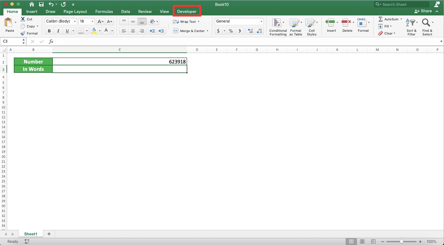
- How to Convert Number to Words in Excel
- Why We Need to Learn About Excel Convert Number to Words?
- How to Convert Number to Words in Excel 2: Various Formulas Combination
- How to Convert Number to Words in Excel 3: Custom Formula (VBA)
- Enable Macro by Checking and Setting Macro Security Setting
- Create the Custom Formula to Convert Number to Words in Excel Using VBA Code
- Use the Formula
- Add-In Download for the Formula to Convert Number to Words in Excel
- How to Convert Number to Words with Currency in Excel
- How to Capitalize Each First Letter in the Result from Converting a Number to Words in Excel: PROPER
- How to Capitalize All Letters in the Result from Converting a Number to Words in Excel: UPPER
- Exercise
- Instruction:
- Additional Note
Convert numbers into words
Excel doesn’t have a default function that displays numbers as English words in a worksheet, but you can add this capability by pasting the following SpellNumber function code into a VBA (Visual Basic for Applications) module. This function lets you convert dollar and cent amounts to words with a formula, so 22.50 would read as Twenty-Two Dollars and Fifty Cents. This can be very useful if you’re using Excel as a template to print checks.
If you want to convert numeric values to text format without displaying them as words, use the TEXT function instead.
Note: Microsoft provides programming examples for illustration only, without warranty either expressed or implied. This includes, but is not limited to, the implied warranties of merchantability or fitness for a particular purpose. This article assumes that you are familiar with the VBA programming language, and with the tools that are used to create and to debug procedures. Microsoft support engineers can help explain the functionality of a particular procedure. However, they will not modify these examples to provide added functionality, or construct procedures to meet your specific requirements.
Create the SpellNumber function to convert numbers to words
Use the keyboard shortcut, Alt + F11 to open the Visual Basic Editor (VBE).
Note: You can also access the Visual Basic Editor by showing the Developer tab in your ribbon.
Click the Insert tab, and click Module.
Copy the following lines of code.
Note: Known as a User Defined Function (UDF), this code automates the task of converting numbers to text throughout your worksheet.
Paste the lines of code into the Module1 (Code) box.
Press Alt + Q to return to Excel. The SpellNumber function is now ready to use.
Note: This function works only for the current workbook. To use this function in another workbook, you must repeat the steps to copy and paste the code in that workbook.
Use the SpellNumber function in individual cells
Type the formula =SpellNumber( A1) into the cell where you want to display a written number, where A1 is the cell containing the number you want to convert. You can also manually type the value like =SpellNumber(22.50).
Press Enter to confirm the formula.
Save your SpellNumber function workbook
Excel cannot save a workbook with macro functions in the standard macro-free workbook format (.xlsx). If you click File > Save. A VB project dialog box opens. Click No.
You can save your file as an Excel Macro-Enabled Workbook (.xlsm) to keep your file in its current format.
Click File > Save As.
Click the Save as type drop-down menu, and select Excel Macro-Enabled Workbook.
Источник
Format numbers as text
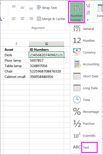
If you want Excel to treat certain types of numbers as text, you can use the text format instead of a number format. For example, If you are using credit card numbers, or other number codes that contain 16 digits or more, you must use a text format. That’s because Excel has a maximum of 15 digits of precision and will round any numbers that follow the 15th digit down to zero, which probably isn’t what you want to happen.
It’s easy to tell at a glance if a number is formatted as text, because it will be left-aligned instead of right-aligned in the cell.
Select the cell or range of cells that contains the numbers that you want to format as text. How to select cells or a range.
Tip: You can also select empty cells, and then enter numbers after you format the cells as text. Those numbers will be formatted as text.
On the Home tab, in the Number group, click the arrow next to the Number Format box, and then click Text.
Note: If you don’t see the Text option, use the scroll bar to scroll to the end of the list.
To use decimal places in numbers that are stored as text, you may need to include the decimal points when you type the numbers.
When you enter a number that begins with a zero—for example, a product code—Excel will delete the zero by default. If this is not what you want, you can create a custom number format that forces Excel to retain the leading zero. For example, if you’re typing or pasting ten-digit product codes in a worksheet, Excel will change numbers like 0784367998 to 784367998. In this case, you could create a custom number format consisting of the code 0000000000, which forces Excel to display all ten digits of the product code, including the leading zero. For more information about this issue, see Create or delete a custom number format and Keep leading zeros in number codes.
Occasionally, numbers might be formatted and stored in cells as text, which later can cause problems with calculations or produce confusing sort orders. This sometimes happens when you import or copy numbers from a database or other data source. In this scenario, you must convert the numbers stored as text back to numbers. For more information, see Convert numbers stored as text to numbers.
You can also use the TEXT function to convert a number to text in a specific number format. For examples of this technique, see Keep leading zeros in number codes. For information about using the TEXT function, see TEXT function.
Источник
How to Convert Number to Words in Excel


In this tutorial, you will learn completely how to convert a number to words in excel.
When processing numbers in excel, especially if they are financial related numbers, we sometimes need the numbers’ words form. Unfortunately, there isn’t a built-in excel formula that can help us to convert our numbers to their word form directly. However, there are some alternative methods we can implement which will give us similar results.
Want to know what are those methods in excel to convert our numbers to words properly? Read all parts of this tutorial.
Disclaimer: This post may contain affiliate links from which we earn commission from qualifying purchases/actions at no additional cost for you. Learn more
Want to work faster and easier in Excel? Install and use Excel add-ins! Read this article to know the best Excel add-ins to use according to us!
Why We Need to Learn About Excel Convert Number to Words?
If the numbers you want to convert to words are small numbers, then you can use VLOOKUP to do it.
However, before you write the VLOOKUP, you need to create a table that consists of numbers and their word forms. The table will then become the reference where VLOOKUP will find the word form of your number.
Generally, the writing form of your VLOOKUP for this number conversion process will become like this.
We input our number as the lookup reference value and the column index of the words form in our reference table. We input FALSE as the VLOOKUP search mode because we want the exact word form for our number (if we input TRUE, then VLOOKUP may take the wrong word form for our number because of its approximate search mode).
To better understand the VLOOKUP method implementation, see the example below.
Let’s say we want to convert this number into words.
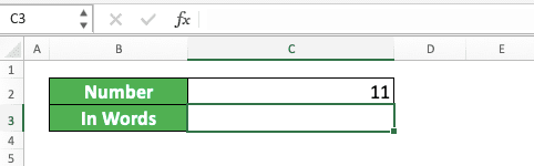
How to do the conversion? Using the VLOOKUP method, we need to create a number-words table first as the VLOOKUP reference table.
To make the display cleaner, it is better if we create the table on a separate sheet. For the example, we create a reference table like this for our VLOOKUP.
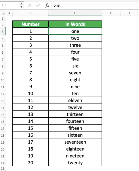
If you need to, you can create a much bigger reference table to be able to convert more numbers!
After you have the table ready, just write VLOOKUP in the cell where you want the words form of your number. Input the number you want to convert, the reference table, the words column index, and FALSE to the VLOOKUP.
Here is the VLOOKUP writing to convert the number in the example.
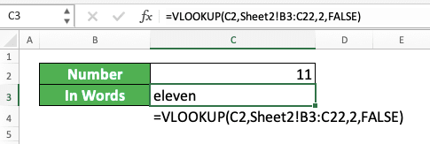
As you have already created the reference table, you can use it later when you have other numbers to convert!
Admittedly, this method can only convert a small selection of numbers. What if you have numbers with the value of millions or more? If that is the case, then you should use one of the two methods we will discuss next instead.
How to Convert Number to Words in Excel 2: Various Formulas Combination
Using multiple formulas in one writing, we can also convert our number to its word form in excel. The formula writing, however, is quite long so you might need to copy the formula from here instead of writing it yourself 🙂
Just so you know, we don’t write the formula we will show below ourselves. The credit all goes to an Excel Forum user with the Id HaroonSid who managed to get this gem out. We edit the formula a little bit so it will translate a number into pure words without currency terms.
Here is the formula that HaroonSid has formulated to solve the number to words conversion problem in excel. This assumes your number is in the B2 cell. Therefore, you need to change the B2 cell coordinate there if you put your number in another cell.
Here, what we can tell is the formula uses CHOOSE as its core to converts the number in B2 to words. Mostly, it convert the number writing format using the TEXT formula first before separating its parts using MID.
From the MID result, CHOOSE will determine the correct word form for the part of the number. It uses the logic with other formulas help like SUBSTITUTE and IF to convert each part of our number into words.
For the implementation example of the formula writing, take a look at the screenshot below.
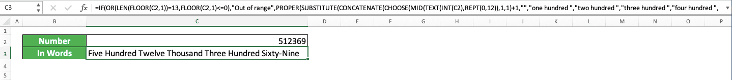
As you can see, we manage to convert our number to words using the formula!
How to Convert Number to Words in Excel 3: Custom Formula (VBA)
If you don’t use the two methods we have already discussed, then there is one more method you can try. For this method, we use VBA code to create a custom formula that can convert our numbers into words easily.
To use this method, however, you need to enable Macro first in your excel workbook so we can use VBA. From there, you must copy the VBA code we have prepared below to your workbook before you can utilize the formula.
To make it easier for you, we divide the discussion for this method into three parts. Those parts are the macro enablement, the VBA code copy process, and the usage of the formula. We will discuss each part in a step-by-step style.
Enable Macro by Checking and Setting Macro Security Setting
To be able to use a custom formula from a VBA code in excel, you need to permit macro. Therefore, we need to ensure its correct permission setting first by doing the following steps.
- Click File from the menu tab (In Mac, click Excel on the top left of your screen)
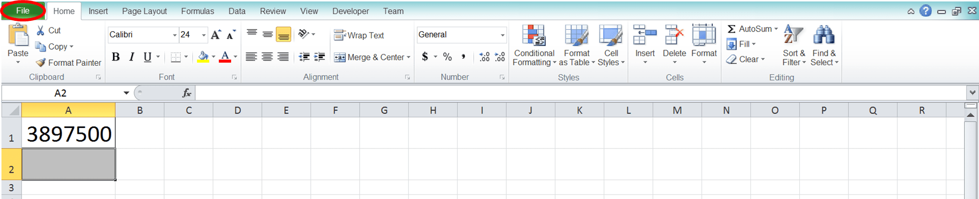
Click Options (In Mac, click Preferences)

Click Trust Center (In Mac, click Security. After that, please proceed to step 6)
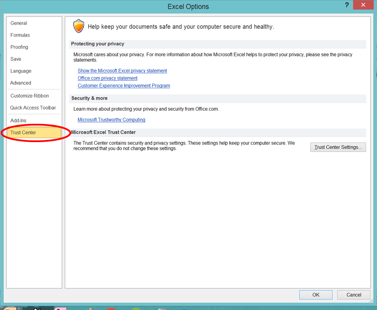
Click Trust Center Settings.

Click Macro Settings
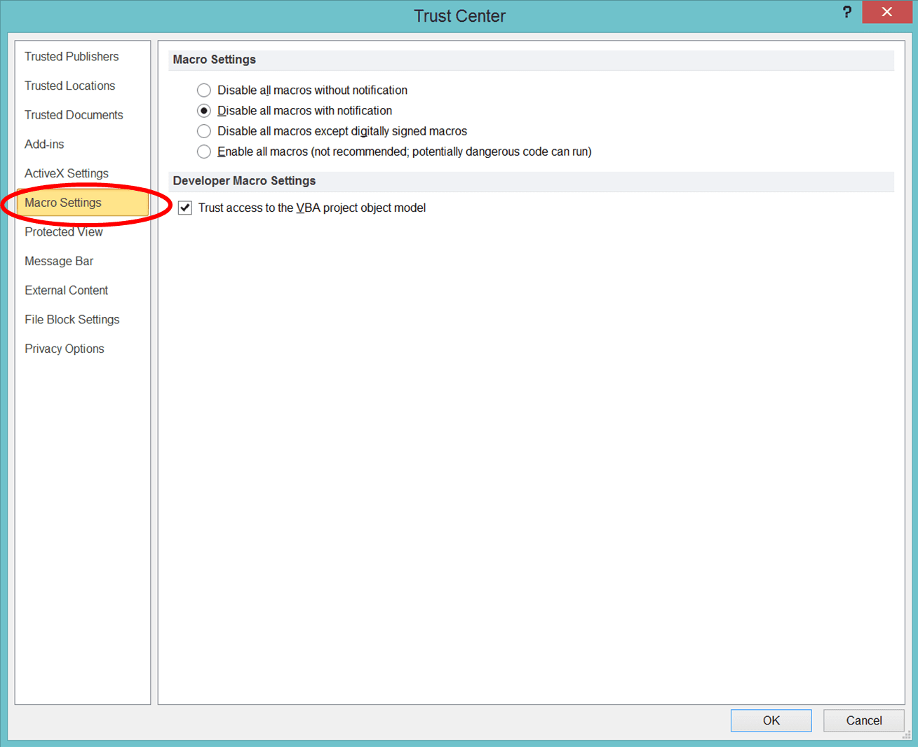
Choose Enable All Macros
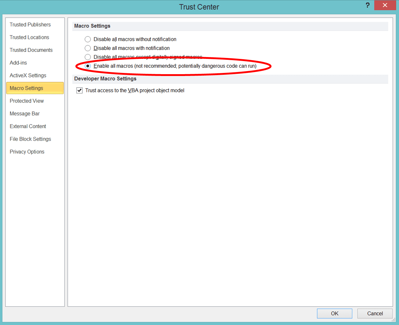
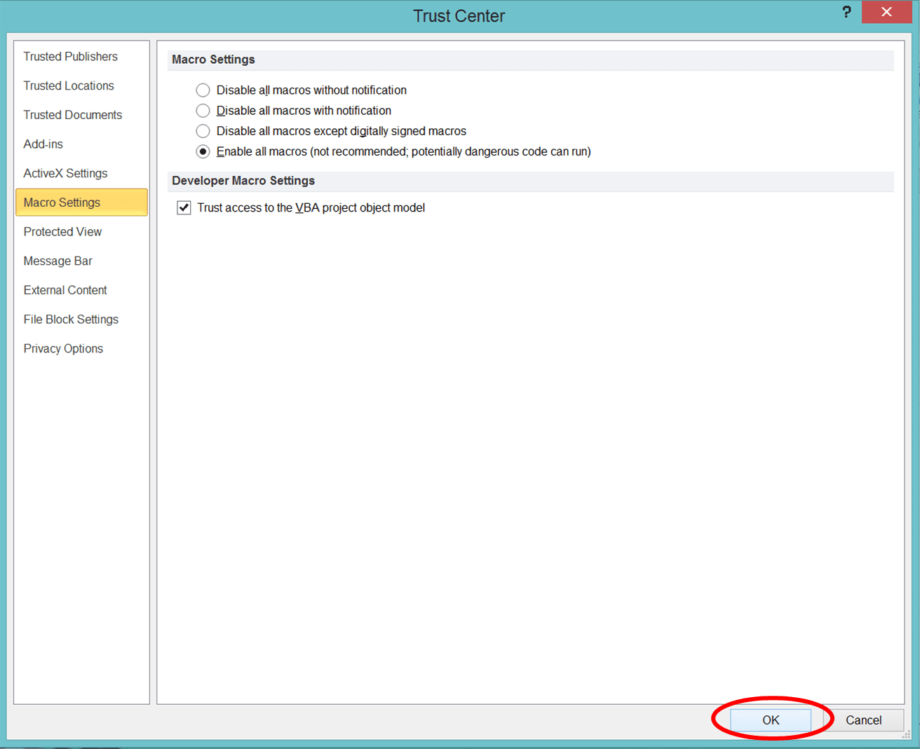
Click OK and OK

Click File and then Save As
On the Save as Type:dropdown, choose Excel Macro-Enabled Workbook
Name your file in the File Name: text box
Click Save
Create the Custom Formula to Convert Number to Words in Excel Using VBA Code
After setting our macro permission, it is time to create the formula using VBA.
- Press Alt and F11 (Option + F11 atau Option + Fn + F11 di Mac) at the same time on your keyboard
- Right-click on “VBA Project…”
Highlight Insert with your pointer and click Module
Double Click on the Module that comes up. Paste this code on the right side of the VBA editor screen
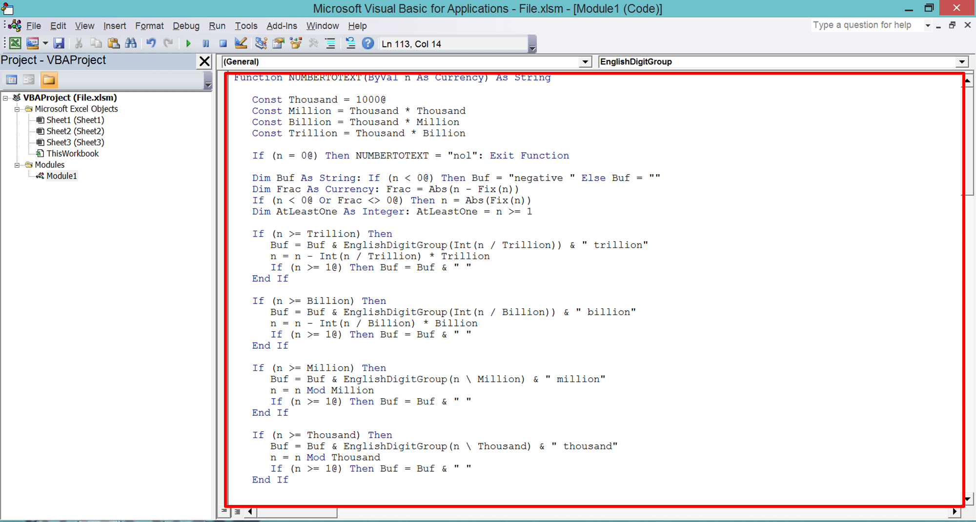
Function NUMBERTOTEXT(ByVal n As Currency) As String В В
Const Thousand = 1000@ В В
Const Million = Thousand * Thousand В В
Const Billion = Thousand * Million В В
Const Trillion = Thousand * Billion В В
If (n = 0@) Then NUMBERTOTEXT = «zero»: Exit Function В В
Dim Buf As String: If (n 0@) Then n = Abs(Fix(n)) В В
Dim AtLeastOne As Integer: AtLeastOne = n >= 1 В В
If (n >= Trillion) Then В В В
Buf = Buf & EnglishDigitGroup(Int(n / Trillion)) & » trillion» В В В
n = n — Int(n / Trillion) * Trillion В В В
If (n >= 1@) Then Buf = Buf & » » В В
End If В В
If (n >= Billion) Then В В В
Buf = Buf & EnglishDigitGroup(Int(n / Billion)) & » billion» В В В
n = n — Int(n / Billion) * Billion В В В
If (n >= 1@) Then Buf = Buf & » » В В
End If В В
If (n >= Million) Then В В В
Buf = Buf & EnglishDigitGroup(n Million) & » million» В В В
n = n Mod Million В В В
If (n >= 1@) Then Buf = Buf & » » В В
End If В В
If (n >= Thousand) Then В В В
Buf = Buf & EnglishDigitGroup(n Thousand) & » thousand» В В В
n = n Mod Thousand В В В
If (n >= 1@) Then Buf = Buf & » » В В
End If В В
If (n >= 1@) Then В В В
Buf = Buf & EnglishDigitGroup(n) В В
End If В В
If (Frac = 0@) Then В В В
Buf = Buf В В
ElseIf (Int(Frac * 100@) = Frac * 100@) Then В В В
If AtLeastOne Then Buf = Buf & » » В В В
Buf = Buf & Format$(Frac * 100@, «00») & «/100» В В
Else В В В
If AtLeastOne Then Buf = Buf & » » В В В
Buf = Buf & Format$(Frac * 10000@, «0000») & «/10000» В В
End If В В
NUMBERTOTEXT = Buf
End Function
Private Function EnglishDigitGroup(ByVal n As Integer) As String В В
Const Hundred = «hundred» В В
Const One = «one » В В
Const Two = «two » В В
Const Three = «three » В В
Const Four = «four » В В
Const Five = «five » В В
Const Six = «six » В В
Const Seven = «seven » В В
Const Eight = «eight » В В
Const Nine = «nine » В В
Dim Buf As String: Buf = «» В В
Dim Flag As Integer: Flag = False В В
Select Case (n 100) В В В
Case 0: Buf = «»: Flag = False В В В
Case 1: Buf = One & Hundred: Flag = True В В В
Case 2: Buf = Two & Hundred: Flag = True В В В
Case 3: Buf = Three & Hundred: Flag = True В В В
Case 4: Buf = Four & Hundred: Flag = True В В В
Case 5: Buf = Five & Hundred: Flag = True В В В
Case 6: Buf = Six & Hundred: Flag = True В В В
Case 7: Buf = Seven & Hundred: Flag = True В В В
Case 8: Buf = Eight & Hundred: Flag = True В В В
Case 9: Buf = Nine & Hundred: Flag = True В В
End Select В В
If (Flag <> False) Then n = n Mod 100 В В
If (n > 0) Then В В В
If (Flag <> False) Then Buf = Buf & » » В В
Else В В В
EnglishDigitGroup = Buf В В В
Exit Function В В
End If В В
Select Case (n 10) В В В
Case 0, 1: Flag = False В В В
Case 2: Buf = Buf & «twenty»: Flag = True В В В
Case 3: Buf = Buf & «thirty»: Flag = True В В В
Case 4: Buf = Buf & «forty»: Flag = True В В В
Case 5: Buf = Buf & «fifty»: Flag = True В В В
Case 6: Buf = Buf & «sixty»: Flag = True В В В
Case 7: Buf = Buf & «seventy»: Flag = True В В В
Case 8: Buf = Buf & «eighty»: Flag = True В В В
Case 9: Buf = Buf & «ninety»: Flag = True В В
End Select В В
If (Flag <> False) Then n = n Mod 10 В В
If (n > 0) Then В В В
If (Flag <> False) Then Buf = Buf & » » В В
Else В В В
EnglishDigitGroup = Buf В В В
Exit Function В В
End If В В
Select Case (n) В В В
Case 0: В В В
Case 1: Buf = Buf & «one» В В В
Case 2: Buf = Buf & «two» В В В
Case 3: Buf = Buf & «three» В В В
Case 4: Buf = Buf & «four» В В В
Case 5: Buf = Buf & «five» В В В
Case 6: Buf = Buf & «six» В В В
Case 7: Buf = Buf & «seven» В В В
Case 8: Buf = Buf & «eight» В В В
Case 9: Buf = Buf & «nine» В В В
Case 10: Buf = Buf & «ten» В В В
Case 11: Buf = Buf & «eleven» В В В
Case 12: Buf = Buf & «twelve» В В В
Case 13: Buf = Buf & «thirteen» В В В
Case 14: Buf = Buf & «fourteen» В В В
Case 15: Buf = Buf & «fifteen» В В В
Case 16: Buf = Buf & «sixteen» В В В
Case 17: Buf = Buf & «seventeen» В В В
Case 18: Buf = Buf & «eighteen» В В В
Case 19: Buf = Buf & «nineteen» В В
End Select В В
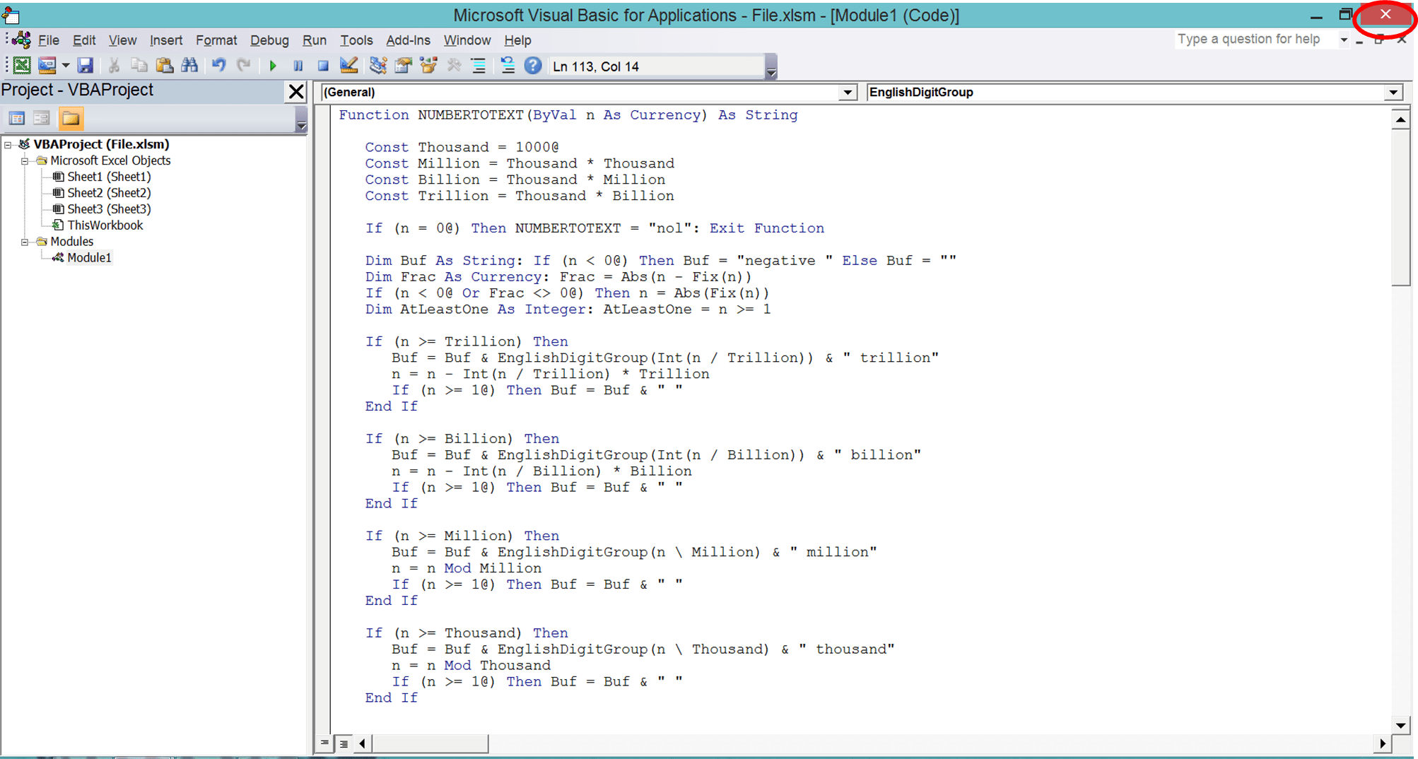
Click on the X mark in the red box on the top right to close your VBA editor. The formula is now ready to use!
Use the Formula
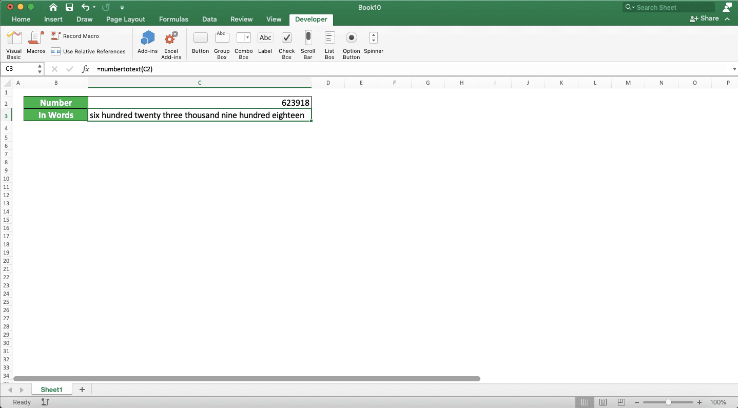
After inputting the VBA code to create the formula, it is time to use it!
- Type an equal sign ( = ) in the cell where you want to put the words form of your number

Type NUMBERTOTEXT (can be with large and small letters) and an open bracket sign after =
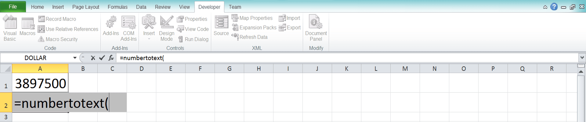
Input the number you want to convert to words/cell coordinate where it is
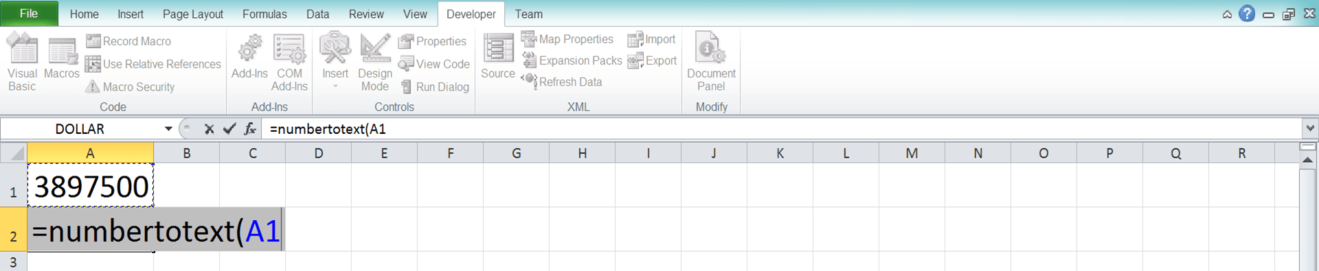
Type a close bracket sign


Add-In Download for the Formula to Convert Number to Words in Excel
Got confused when you need to paste the VBA code for the formula to convert your number to words? Then, you can just download the excel add-in we have created from the code here!
After you download it, just activate the add-in in your excel workbook. For that, you need to display the Developer tab first in your excel if you haven’t.
To display the Developer tab, go to Files > Options > Customize Ribbon (In Mac, go to Excel > Preferences > Ribbon & Toolbar > Ribbon Tab). Then, on the right box, make sure the Developer check box is checked.
After the Developer tab is there in your excel workbook, follow these steps. Make sure you have downloaded the add-in we provide earlier and put it somewhere on your computer.
- Go to the Developer tab
Click the Excel Add-Ins button


Done! Now, you can use the NUMBERTOTEXT formula to convert your number into words!
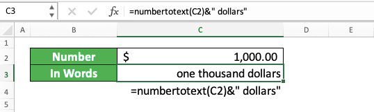
How to Convert Number to Words with Currency in Excel
As number conversion to words is usually done for financial numbers, you may need to add currency in the conversion result. For that, you can use CONCATENATE, CONCAT, or the ampersand symbol (&) to add the currency word.
For example, if you use the NUMBERTOTEXT custom formula to convert your number, then the writing will be like this. This assumes you want to add the “dollars” currency word behind the conversion result. We use the ampersand symbol to add the currency word for this.
Don’t forget to add a space in front of the “dollars” word.
Here is the implementation example of this method in excel.
Quite easy, isn’t it?
How to Capitalize Each First Letter in the Result from Converting a Number to Words in Excel: PROPER
If you need to capitalize the first letter of each word from the number conversion, then you need a specific formula. That formula is PROPER.
You can envelop the number conversion formula you use with PROPER to do the capitalization. Generally, here is the general writing form of that, assuming you use the NUMBERTOTEXT formula.
Simple, isn’t it? And here is the example of the PROPER usage for the conversion result.

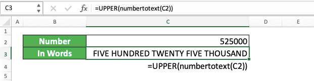
How to Capitalize All Letters in the Result from Converting a Number to Words in Excel: UPPER
What about if we want to capitalize all the letters instead? For that, you should use UPPER!
The way to use UPPER here is the same as the way we use PROPER earlier. Here is the general writing form of the UPPER implementation to our NUMBERTOTEXT formula.
And here is the implementation example of that writing.
Exercise
After you have learned how to convert numbers to words in excel using various methods, let’s do an exercise! We make this exercise so you can understand more practically about this tutorial topic.
Download the exercise file from the following link and do the instructions. Download the answer if you have done the exercise and sure about the results!
Link to the exercise file:
Download here
Instruction:
Additional Note
- The NUMBERTOTEXT formula cannot be used to convert decimal digits you have in your number to words
- If you input the VBA code manually, then you won’t find the NUMBERTOTEXT formula if you create a new workbook. You must use the add-in for that or you must paste the VBA code to create the NUMBERTOTEXT formula again
Related tutorials you should learn too:
Источник
Behold… Pete’s creation!!!!!!!!!!

DON’T RUN AWAY JUST YET!
Don’t worry if this looks a bit intimidating; you don’t need to understand this to use it. We only need to know how to integrate it into our spreadsheets.
SCROLL DOWN TO DOWNLOAD THE WORKBOOK & CHECK OUT THE POWER QUERY SOLUTION TO THIS (sent to us by our wonderful community)
Let’s look at some examples


This formula is quite complex, having to account for such instances of where it sees values such as “Eleven” (as opposed to “One and One”), “Twenty”, “Thirty”, and weather to say things like “Hundred” versus “Hundred and” something.
The combination of numbers to words can be quite daunting.
Changing the Currency and Decimal Usage
Suppose you need to update this formula to work with US dollars and you don’t require the decimal places.
If you look at the very end of the formula, you will see the portion that is responsible for the decimal places.
&RIGHT(TEXT(B3,"000000000.00"),2)&"/100"
If you do not require decimal places to be displayed, erase this portion of the formula.
For the currency type, change the portion labeled “Euro” to “USD” or “CAD” or whatever currency designation you wish.

Let’s see how that appears after our little formula tweak.

How to apply the formula to many cells
Suppose you have a spreadsheet and you wish to enter a number in cell B4 and have the formula answer appear in the cell directly to the right in cell C4.
We need to make sure that none of the cell references change when copying the formula to a new location.
- Place your cursor on the cell holding the original formula and press F2 to enable edit mode (or click in the Formula Bar).
- Select the entire formula by pressing CTRL-A (or manually highlighting the formula. CTRL-A is faster and more accurate.)
- Press CTRL-C to copy the formula.
- Press the ESC (Escape) key to back out of edit mode.
- Switch to the location and cell you wish to use this formula and press F2 to enable edit mode.
- Press CTRL-V to paste the formula into the new cell.
We’re not quite there yet because all the cell references are pointing to cell B3. If your data entry cell is in fact cell B3, you are ready to go. If not, we need to update the cell references to point to the proper data entry location.
Because our original formula was looking at cell B3 for the number and we wish to enter our number in cell B4, we will now perform the following steps to adjust our cell references:
- Place your cursor on the cell holding the pasted formula and press F2 to enable edit mode (or click in the Formula Bar).
- Remove the equals sign (=) from the beginning of the formula.
- Press ENTER. We now have just a massive amount of text in the cell.
- Press CTRL-H to open the Find/Replace dialog box.
- In the “Find what:” field, enter “B3” (no double-quotes).
- In the “Replace with:” field, enter “B4” (no double-quotes).
- Press the “Replace All” button.

Restore the equals sign to the beginning of the formula from where we removed it earlier in step 2.
Running it through some tests
To test the formula quickly and over multiple iterations, select cell B4 and enter the following formula.
=RANDBETWEEN(1,2000000)This formula will generate a random number between 1 and 2-million each time the sheet recalculates.

You can force a recalculation by pressing the F9 key on the keyboard or pressing Formulas (tab) -> Calculation (group) -> Calculate Now.

To see several examples simultaneously, select cells B4 and C4 and pull the Fill Series handle down several rows. This will generate several random numbers and their text counterparts.

Bonus Modification
If you decide to not display the fractional side of the number, the above modification simply removes the fractional values without any rounding operation.
If you would like to round the input to the nearest whole number, implement the following steps:
- Place your cursor on the cell holding the pasted formula and press F2 to enable edit mode (or click in the Formula Bar).
- Remove the equals sign (=) from the beginning of the formula.
- Press ENTER. We now have just a massive amount of text in the cell.
- Press CTRL-H to open the Find/Replace dialog box.
- In the “Find what:” field, enter “B3” (no double-quotes).
- In the “Replace with:” field, enter “ROUND(B3,0)” (no double-quotes).
- Press the “Replace All” button.

Restore the equals sign to the beginning of the formula from where we removed it earlier in step 2.
Don’t forget to change the B3 reference to whichever cell you are performing the data entry.
Are you curious as to how all this works?
This formula relies on the use of four key functions:
- LEFT
- MID
- TEXT
- CHOOSE
It’s not necessary to dissect every component of the formula, we only need to decipher the first bit highlighted below.

CHOOSE(LEFT(TEXT(B3),"000000000.00"))+1,,"One","Two","Three",
"Four","Five","Six","Seven","Eight","Nine")
&IF(--LEFT(TEXT(B3),"000000000.00"))=0,,IF(AND(--MID(TEXT(B3),"000000000.00"),
2,1)=0,--MID(TEXT(B3),"000000000.00"),3,1)=0)," Hundred"," Hundred and "))
Once we have this portion figured out we’ll be able to figure out the remainder of the formula since it is very much a repeated operation.
The LEFT Function
The purpose of the LEFT function is to extract a specific number of characters from the text starting from the left side. The structure of the LEFT function is as follows.
=LEFT(text, [num_chars])The parameter “text” refers to the cell holding the input, while “[num_chars]” indicates the number of characters to extract. Because the “[num_chars]” parameter is optional, skipping this parameter will result in a default extraction of 1 character.
The MID Function
The purpose of the MID function is to extract a specific number of characters from the text starting from a specific character position (counting from the left side). The structure of the MID function is as follows.
=MID(text, start_num, num_chars)The parameter “text” refers to the cell holding the input; the parameter “start_num” indicates the position to begin text extraction (counting from the left side), while “num_chars” indicates the number of characters to extract.
The TEXT Function
The purpose of the TEXT function is to represent a cell’s information with specific formatting. The structure of the TEXT function is as follows.
=TEXT(value, format_text)Normally, formatting is applied to a cell through traditional cell formatting controls.

The TEXT function applies formatting (fancy word alert) formulaically. This way, we can change the formatting of information dynamically based on the need of the moment.
EXAMPLE: Suppose you have a calculation that needs to reflect U.S. Dollars or Euros depending on a country selection. The formula could look something like the following:
=IF(Country=”USA”, TEXT(Sale, ”$#,##0.00”), TEXT(Sale, “€#,##0.00”))If the user selects USA (cell A2) , they get the total sales represented by a “$” sign (cell C4) . If the user selects any other country, the total sales is represented by a “€” symbol.

This function relies on a cell named “Country” (cell A2) where a user may select a country from a Data Validation dropdown list, and a cell named “Sale” (cell A9) that may hold something like a SUM function that adds all the sales together.
In our specific example, the function…
=TEXT(B3,”000000000.00”)…pads the input number with leading zeroes. By counting the leading zeroes, the formula will be able to determine if the number is in the hundreds, thousands, or millions.
If a user inputs a number, such as 123456.78, the TEXT function will interpret the number as 000123456.78. The three leading zeroes indicates a number in the thousands.
The CHOOSE Function
The CHOOSE function is used to simplify multiple nested IF functions that are examining the same data. CHOOSE is especially useful when working with indexes.
The purpose of the CHOOSE function is to select a value from a built-in list of values based on a supplied number.
=CHOOSE(index_num, value1, [value2], …)If we were to extract the first (left-most) number from the input number and give it to the following CHOOSE function, what do you think we would get back from the CHOOSE function?
=CHOOSE(LEFT(B3), “One”, “Two”, “Three”, “Four”, “Five”, “Six”, “Seven”,
“Eight”, “Nine”)
We would see the word version of the extracted number. “2” would yield “Two”, “5” would yield “Five”, etc…
Putting it All Together
In the formula, we are combining all the functions into a single formula, each function performing their respective parts to accomplish the mission.
CHOOSE(LEFT(TEXT(B3,"000000000.00"))+1,,"One","Two","Three",
"Four","Five","Six","Seven","Eight","Nine")
&IF(--LEFT(TEXT(B3,"000000000.00"))=0,,IF(AND(--MID(TEXT(B3,"000000000.00"),
2,1)=0,--MID(TEXT(B3,"000000000.00"),3,1)=0)," Hundred"," Hundred and "))
First we use the TEXT function to turn the number into a “000000000.00” format.
TEXT(B3,"000000000.00")Then, we extract the left-most character form the number.
LEFT(TEXT(B3,"000000000.00"))This will allow us to determine if the returned number is a zero or any other value. This will indicate weather or not our number is in the “millions” range.
Next, we CHOOSE how to represent the extracted value.
CHOOSE(LEFT(TEXT(B3,"000000000.00"))+1,,"One","Two","Three",
"Four","Five","Six","Seven","Eight","Nine")
We then check to see if the value is a zero.
CHOOSE(LEFT(TEXT(B3,"000000000.00"))+1,,"One","Two","Three",
"Four","Five","Six","Seven","Eight","Nine")
&IF(--LEFT(TEXT(B3,"000000000.00"))=0,,
If the value is a zero, then we are not in the millions so we will display nothing.
If the next two digits are zero, then we will display “Hundred”; otherwise, we will display “Hundred and”.
CHOOSE(LEFT(TEXT(B3,"000000000.00"))+1,,"One","Two","Three","Four",
"Five","Six","Seven","Eight","Nine")
&IF(--LEFT(TEXT(B3,"000000000.00"))=0,,IF(AND(--MID(TEXT(B3,"000000000.00"),
2,1)=0,--MID(TEXT(B3,"000000000.00"),3,1)=0)," Hundred"," Hundred and "))
That’s It!
This formula doesn’t rely on any
- VBA
- CTRL-Shift-Enter Array Formulas, or
- Helper Cells
Thank you, Pete for sharing your formula with the Excel community. I’m certain many will find your solution both creative and highly useful.
Practice Workbook
Feel free to Download the Workbook HERE.
![]()
Many thanks to Jim M. for updating the formula for US syntax, Zafar for updating it for billions as well as text as decimal places!
Also many thanks to Abdul Rahman Mohammed for providing the Qatari Riyals (QAR), Indian Rupees (INR) & Bahraini Dinars (BHD) in both absolute and rounded figures.
The reworked versions are available in the downloadable Workbook.
Power Query Solution!
A Power Query solution of transforming numbers to works was sent to us by Kunle SOPEJU.
Check out his Power Query solution HERE.
![]()
Many thanks to Kunle SOPEJU for letting us get creative with Power Query!
Published on: May 16, 2019
Last modified: March 1, 2023


Leila Gharani
I’m a 5x Microsoft MVP with over 15 years of experience implementing and professionals on Management Information Systems of different sizes and nature.
My background is Masters in Economics, Economist, Consultant, Oracle HFM Accounting Systems Expert, SAP BW Project Manager. My passion is teaching, experimenting and sharing. I am also addicted to learning and enjoy taking online courses on a variety of topics.
November 10, 2020
VBA Excel Macros
5,562 Views
Microsoft Excel is surely one of the most used and best-known spreadsheet software. Providing almost infinite possibilities when it comes to calculating and processing data, it can be used to create complex spreadsheets and supports a wide range of functions.
One of the most requested functions is the ability to convert number to words in Excel. Unfortunately, Excel does not currently have such a built-in feature!
But don’t worry, today I will show you step by step how to convert numbers to text using a very simple to use Excel Macro that you can download for free and install in seconds.
🢃 🢃 (Download link is available at the end of this article) 🢃 🢃
Download the Convert Number to Words Excel Macro
So, the first step is to download the VBA Macro. As I said in the introduction, you will find the download link at the end of the article. Don’t worry this Excel macro is totally free, just click the Download Now button and save the “.xla” file to your computer.
Remember, this MS Macro is able to convert not only numbers into words in Excel, but also decimals and money amounts too.
You will even be able to select the currency you want to convert the money amounts to. Of course, all this while respecting the spelling rules for writing numbers.
Examples for spelled out numbers:
- Convert 90 in words : Ninety
- Translate decimal 13.78 in text : Thirteen and seventy-eight hundredths
- Change amount $20.99 in letters : Twenty dollars and ninety-nine cents
What is a .XLA or .XLAM File?
A file with the extension ‘.XLA’ is an Excel add-in file. XLA file types are used to add extra functions and modules to Microsoft Excel. They will open each time Excel is opened.
It contains Macros in VBA code and also other calculations that you can use in Excel worksheet documents.
XLA Macros are developed by a third-party and may be used by Mac and Windows programs for different types of data treatment.
Install the Number in Words Converter Macro to Microsoft Excel
This is the second step you will need to do to be able to convert numbers in Excel. After this step, and thanks to this free VBA Code Excel Macro, your Microsoft spreadsheet software will be equipped with a new function “ConvertNumber” that you will love.
It will save you time and increase your productivity.
In this demo tutorial, we will use Microsoft Excel 2016, but this Macro will work fine with the different versions of Microsoft Office Excel spreadsheets including Excel 2007, 2010, 2013 and 2016.
So let’s install the Macro add-on now :
STEP1
On the top menu, click “File” then “Options”.
Choose the “Add-ins” tab then the button “Go” at the bottom of the “Excel Options” window.

STEP2
Now after clicking the “Go” button, a small window “Add-ins” will open.
Click “Browse” and then select the Excel macro file that you downloaded (.xla file format). Download link available at the end of the article.

Please Note:
You mast put the Macro file in a fixed location on your PC and do not move it to another folder once the macro has been added to MS Excel.
Otherwise, you will not be able to convert numeric into words in Excel using this Macro.
Great, everything is ready now.
Just keep reading, I will explain how to use the Macro to convert numbers, decimals and money amounts in English words.
How to use the macro to converting numbers into letters in Microsoft Excel 2016?
After installing the macro, create a new Excel document.
You will notice that you have a new Function added to your MS Excel, “=ConvertNumber(XX)”.
Ok lets try it now!
Several methods of use are possible:
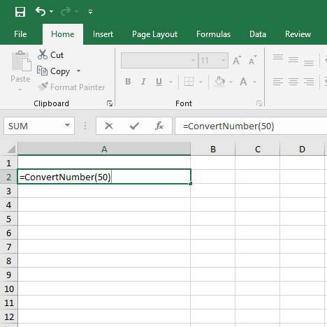
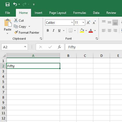
Convert a number to letters directly:
In the cell where you want to get the number converted in words, type “=ConvertNumber(50)” then hit enter.
You will get the conversion result written in words : Fifty
Note: You can also use decimals.
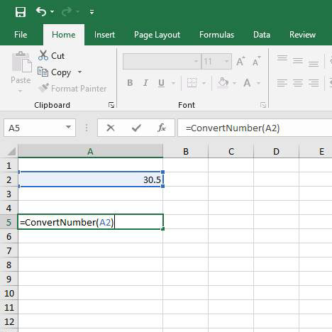
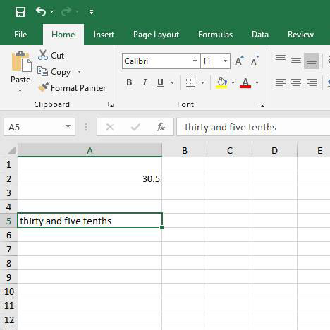
Convert a cell or a range of cells:
Type the Excel formula where you want to spell out number result, and select the cell or the range of cells that you want to convert using your mouse cursor.
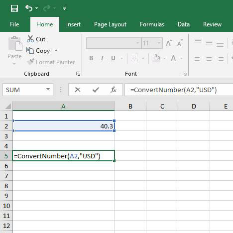
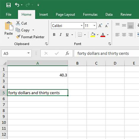
In this example we want to convert the A2 cell, so we will use this Excel formula : “=ConvertNumber(A2)”.
30.5 will be instantly converted to words : Thirty and five tenths.
Super easy, isn’t it?
Convert money amounts to text in Excel:
This is the easiest method to convert money amount in words in Excel using VBA Macros.
To do so, you will need to write this function where you want to convert number to words in Excel : “=ConvertNumber(A2,”USD”)”
As you can see, this formula has 2 parameters:
- A2, the cell you want to convert.
- And “USD”, the currency that you want to convert to it.
The result will be the full amount in USD converted into text. Of course, you can use “EUR” if you want to convert euro amounts.
Conclusion
We hope that this tutorial will help you to convert number in words in Excel easily and without mistakes. Our goal is to help you with Excel Macros and functions. So, feel free to leave your comments below if you have something to add or request. We will do our best to improve this Macro and add more functionality in the future.
[lockercat]
Click Here To Download
[/lockercat]
Excel is a great tool which can be used for data entry, as a database, and to analyze data and create dashboards and reports.
While most of the in-built features and default settings are meant to be useful and save time for the users, sometimes, you may want to change things a little.
Converting your numbers into text is one such scenario.
In this tutorial, I will show you some easy ways to quickly convert numbers to text in Excel.
Why Convert Numbers to Text in Excel?
When working with numbers in Excel, it’s best to keep these as numbers only. But in some cases, having a number could actually be a problem.
Lets look at a couple of scenarios where having numbers creates issues for the users.
Keeping Leading Zeros
For example, if you enter 001 in a cell in Excel, you will notice that Excel automatically removes the leading zeros (as it thinks these are unnecessary).
While this is not an issue in most cases (as you wouldn’t leading zeros), in case you do need these then one of the solutions is to convert these numbers to text.
This way, you get exactly what you enter.
One common scenario where you might need this is when you’re working with large numbers – such as SSN or employee ids that have leading zeros.
Entering Large Numeric Values
Do you know that you can only enter a numeric value that is 15 digits long in Excel? If you enter a 16 digit long number, it will change the 16th digit to 0.
So if you are working with SSN, account numbers, or any other type of large numbers, there is a possibility that your input data is automatically being changed by Excel.
And what’s even worse is that you don’t get any prompt or error. It just changes the digits to 0 after the 15th digit.
Again, this is something that is taken care of if you convert the number to text.
Changing Numbers to Dates
This one erk a lot of people (including myself).
Try entering 01-01 in Excel and it will automatically change it to date (01 January of the current year).
So if you enter anything that is a valid date format in Excel, it would be converted to a date.
A lot of people reach out to me for this as they want to enter scores in Excel in this format, but end up getting frustrated when they see dates instead.
Again, changing the format of the cell from number to text will help keep the scores as is.
Now, let’s go ahead and have a look at some of the methods you can use to convert numbers to text in Excel.
Convert Numbers to Text in Excel
In this section, I will cover four different ways you can use to convert numbers to text in Excel.
Not all these methods are the same and some would be more suitable than others depending on your situation.
So let’s dive in!
Adding an Apostrophe
If you manually entering data in Excel and you don’t want your numbers to change the format automatically, here is a simple trick:
Add an apostrophe (‘) before the number
So if you want to enter 001, enter ‘001 (where there is an apostrophe before the number).
And don’t worry, the apostrophe is not visible in the cell. You will only see the number.

When you add an apostrophe before a number, it will change it to text and also add a small green triangle at the top left part of the cell (as shown in th image). It’s Exel way to letting you know that the cell has a number that has been converted to text.
When you add an apostrophe before a number, it tells Excel to consider whatever follows as text.
A quick way to visually confirm whether the cells are formatted as text or not is to see whether the numbers align to the left out to the right. When numbers are formatted as text, they align to the right by default (as they alight to the left)

Even if you add an apostrophe before a number in a cell in Excel, you can still use these as numbers in calculations
Similarly, if you want to enter 01-01, adding an apostrophe would make sure that it doesn’t get changed into a date.
Although this technique works in all cases, it is only useful if you’re manually entering a few numbers in Excel. If you enter a lot of data in a specific range of rows/columns, use the next method.
Converting Cell Format to Text
Another way to make sure that any numeric entry in Excel is considered a text value is by changing the format of the cell.
This way, you don’t have to worry about entering an apostrophe every time you manually enter the data.
You can go ahead entering the data just like you usually do, and Excel would make sure that your numbers are not changed.
Here is how to do this:
- Select the range or rows/column where you would be entering the data
- Click the Home tab

- In the Number group, click on the format drop down

- Select Text from the options that show up

The above steps would change the default formatting of the cells from General to Text.
Now, if you enter any number or any text string in these cells, it would automatically be considered as a text string.
This means that Excel would not automatically change the text you enter (such as truncating the leading zeros or converting entered numbers into dates)
In this example, while I changed the cell formatting first before entering the data, you can also do this with cells that already have data in them.
But remember that if you already had entered numbers that were changed by Excel (such as removing leading zeros or changing text to dates), that won’t come back. You will have to make that data entry again.
Also, keep in mind that cell formatting can change in case you copy and paste some data to these cells. With regular copy-paste, it also copied the formatting from the copied cells. So it’s best to copy and paste values only.
Using the TEXT Function
Excel has an in-built TEXT function that is meant to convert a numeric value to a text value (where you have to specify the format of the text in which you want to get the final result).
This method is useful when you already have a set of numbers and you want to show them in a more readable format or if you want to add some text as suffix or prefix to these numbers.
Suppose you have a set of numbers as shown below, and you want to show all these numbers as five-digit values (which means to add leading zeros to numbers that are less than 5 digits).

While Excel removes any leading zeros in numbers, you can use the below formula to get this:
=TEXT(A2,"00000")

In the above formula, I have used “00000” as the second argument, which tells the formula the format of the output I desire. In this example, 00000 would mean that I need all the numbers to be at least five-digit long.
You can do a lot more with the TEXT function – such as add currency symbol, add prefix or suffix to the numbers, or change the format to have comma or decimals.
Using this method can be useful when you already have the data in Excel and you want to format it in a specific way.
This can also be helpful in saving time when doing manual data entry, where you can quickly enter the data and then use the TEXT function to get it in the desired format.
Using Text to Columns
Another quick way to convert numbers to text in Excel is by using the Text to Columns wizard.
While the purpose of Text to Columns is to split the data into multiple columns, it has a setting that also allows us to quickly select a range of cells and convert all the numbers into text with a few clicks.
Suppose you have a data set is shown below, and you want to convert all the numbers in columns A into text.
Below are the steps to do this:
- Select the numbers in Column A
- Click the Data tab

- Click on the Text to Columns icon in the ribbon. This will open the text to columns wizard this will open the text to column wizard
- In Step 1 of 3, click the Next button
- In Step 2 of 3, click the Next button
- In Step 3 of 3, under the ‘Column data format’ options, select Text

- Click on Finish
The above steps would instantly convert all these numbers in Column A into text. You notice that the numbers would now be aligned to the right (indicating that the cell content is text).

There would also be a small green triangle at the top left part of the cell, which is a way Excel informs you that there are numbers that are stored as text.
So these are four easy ways that you can use to quickly convert numbers to text in Excel.
In case you only want this for a few cells where you would be manually entering the data, I suggest you use the apostrophe method. If you need to do data entry for more than a few cells, you can try changing the format of the cells from General to Text.
And in case you already have the numbers in Excel and you want to convert them to text, you can use the TEXT formula method or the Text to Columns method I covered in this tutorial.
I hope you found this tutorial useful.
Other Excel tutorials you may also like:
- Convert Text to Numbers in Excel
- How to Convert Serial Numbers to Dates in Excel
- Convert Date to Text in Excel – Explained with Examples
- How to Convert Formulas to Values in Excel
- Convert Time to Decimal Number in Excel
- How to Convert Inches to MM, CM, or Feet in Excel?
- Convert Scientific Notation to Number or Text in Excel
- Separate Text and Numbers in Excel