Freeze the row in excel - Word и Excel - помощь в работе с программами

Freeze panes to lock rows and columns

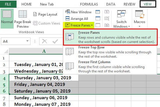
To keep an area of a worksheet visible while you scroll to another area of the worksheet, go to the View tab, where you can Freeze Panes to lock specific rows and columns in place, or you can Split panes to create separate windows of the same worksheet.

Freeze rows or columns

Freeze the first column

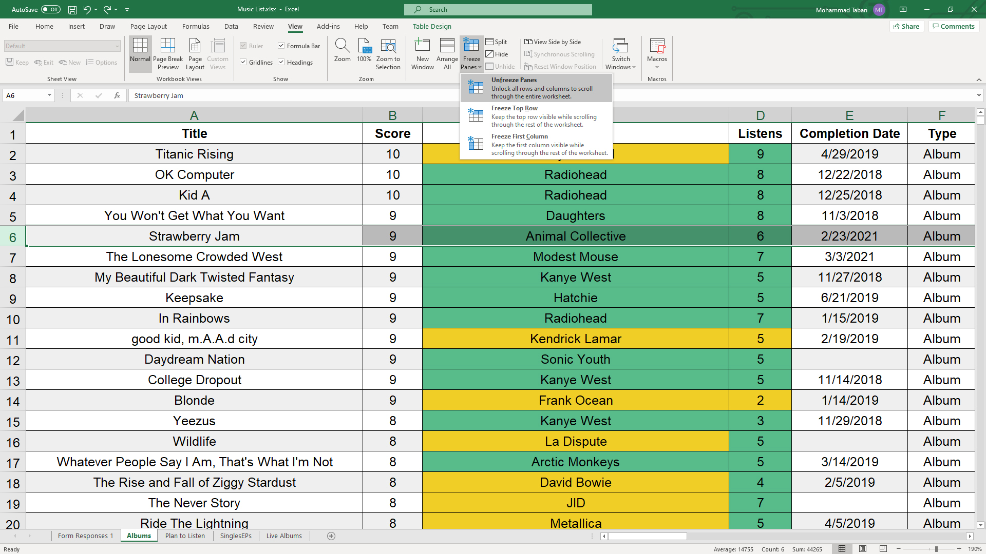
Select View > Freeze Panes > Freeze First Column.

The faint line that appears between Column A and B shows that the first column is frozen.

Freeze the first two columns

Select the third column.
Select View > Freeze Panes > Freeze Panes.

Freeze columns and rows

Select the cell below the rows and to the right of the columns you want to keep visible when you scroll.
Select View > Freeze Panes > Freeze Panes.

Unfreeze rows or columns

On the View tab > Window > Unfreeze Panes.

Note: If you don’t see the View tab, it’s likely that you are using Excel Starter. Not all features are supported in Excel Starter.

Need more help?

You can always ask an expert in the Excel Tech Community or get support in the Answers community.

Freeze First Row

This feature could be used to freeze a particular row or header that you would need to refer every time while working on excel. In this option only the top row will freeze.

Open the sheet where in you want to freeze any row / header, as an example we would like to freeze the top row highlighted in yellow

Now, navigate to the “View” tab in the Excel Ribbon as shown in above image
Click on the “Freeze Panes” button

Select “Freeze Top Row” option

If you would like to freeze any other row, then scroll down and make that row appear as first in your sheet and then repeat Step 2 to 4.

That’s it. You are all set now. As seen in above image you can now scroll to any corner of the page and you would see that the top row remains intact all the time without any change.

Please note that this option works as long as first row in excel is the one that you really want to freeze. If you have scrolled in the middle of the sheet and Row 30 is appearing as first row, then this option would freeze Row 30 and not Row 1.

Additionally, if you are geek and would like to do it directly using a keyboard shortcut, then please press “Alt + W” followed by “F” and then “R”. Please note that this is not an in-built shortcut, rather it’s the same thing from keyboard as we do from mouse.

Freeze First Column

This feature could be used to freeze a particular column that you would need to refer while working on excel. In this option only the first column will freeze.

Open the sheet where in you want to freeze the column, as an example we would like to freeze the column A – Product

Now, navigate to the “View” tab in the Excel Ribbon as shown in above image
Click on the “Freeze Panes” button

Select “Freeze First Column” option

If you would like to freeze any other column, then move right or left and make that column appear as first in your sheet and then repeat Step 2 to 4.

That’s it. You are all set now. As seen in above image you can now move to most right corner of the page and you would see that the first column sticks there. Please note that this option works as long as first column in excel is the one that you really want to freeze. If you have shifted right in the middle of the sheet and Column M is appearing as first row, then this option would freeze Column M and not Column A.

If you would like to do it directly using a keyboard shortcut, then please press “Alt + W” followed by “F” and then “C”. Please note that this is not an in-built shortcut, rather it’s the same thing from keyboard as we do from mouse.

Freeze Panes

This feature could be used to freeze multiple rows, columns or both at the same time. However, this could be done only for the consecutive rows or columns.

Freeze Panes – Multiple Rows

Open the sheet where in you want to freeze the multiple rows, keep the first row on top and click after the last row till where you want to freeze, as an example we would like to freeze from Row 1 to Row 13 so we will click on Row 14

Now, navigate to the “View” tab in the Excel Ribbon as shown in above image
Click on the “Freeze Panes” button

Select “Freeze Panes” option

That’s it. You are all set now. As seen in above image you can now scroll down and Row 1 to Row 13 will be kept intact without any changes. You can select the range of rows from middle as well like – Row 13 to Row 30, however to do so you will have to ensure that you scroll up and keep Row 13 as your first row in the sheet and repeat the steps listed above. However, be careful as doing so some of your rows (i.e. the ones before Row 13) will be hidden.

Freeze Panes – Multiple Columns

Open the sheet where in you want to freeze the multiple columns, keep the first column to the left and click next to the last column till where you want to freeze, as an example we would like to freeze from Column A to E, so we will click on Column F

Now, navigate to the “View” tab in the Excel Ribbon as shown in above image
Click on the “Freeze Panes” button

Select “Freeze Panes” option

That’s it. You are all set now. As seen in above image you can now move towards right and Column A to E will be kept intact without any changes. You can select the range of columns from middle as well like – Column F to Column L, however to do so you will have to ensure that you move to the left and keep Column F as your first column in the sheet and repeat the steps listed above. However, be careful as doing so some of your columns (i.e. the ones before Column E) will be hidden.

Freeze Panes – Multiple Rows and Columns both

If you have followed the post till now, then you would have already figured out how this has to be done. Yes, you are right we are going to club both the above listed approaches here. Follow us below:

Open the sheet where in you want to freeze the multiple rows and columns, keep the first row on top and first column to the left then click next to the cell of the last column and row till where you want to freeze, as an example we would like to freeze from Row 1 to 13 and Column A to E, so we will click on Cell F14

Now, navigate to the “View” tab in the Excel Ribbon as shown in above image
Click on the “Freeze Panes” button

Select “Freeze Panes” option

That’s it. You are all set now. As seen in above image you can now scroll down and Row 1 to 13 will remain intact and likewise you can move towards right and Column A to E will be kept intact without any changes. You can select the range of columns from middle as well like – Row 17 to 27 and Column F to L, however to do so you will have to ensure that you scroll up and keep Row 17 as your first row and keep Column F as your first column in the sheet and repeat the steps listed above. Be careful here as rows before Row 17 and columns before column F will be hidden.

Unfreeze Panes:

If you have frozen the wrong rows and columns, then you could easily undo it by using “Unfreeze Panes” option. This would remove all the frozen rows and or columns in your excel. This will also work if you have received the sheet from someone else and you are not able to see all the rows and columns despite of removing all filters and unhiding rows columns. To unfreeze panes –

Open the sheet wherein you want to unfreeze rows and or columns
Now, navigate to the “View” tab in the Excel Ribbon
Click on the “Freeze Panes” button

Select “Unfreeze Panes” option as shown above

With this all the rows and or columns would unfreeze, as shown in above image. Please note that you would not see the “Unfreeze Panes” option if there are not any frozen rows columns. This option would be available only and only when there is some row and or column frozen already.

If you would like to unfreeze panes it directly using a keyboard shortcut, then please press “Alt + W” followed by “F” and then again “F”. Please note that this is not an in-built shortcut, rather it’s the same thing from keyboard as we do from mouse.

Freeze panes versus Splitting Panes:

Excel also provides you an excellent option to Split Panes which divides the window into different panes that each pane scrolls separately. This option is present in Excel Ribbon, View tab next to Freeze Option.

So as visible in the above image after using split option the content of same sheet is visible in 4 separate panes and all panes have their different scroll options.

We personally trust and use Freeze option much than Split, as Freeze allows you to limit the data movement by freezing it rather than adding multiple views of same data wherein you easily get distracted and confused while data entry.

Is Freeze Pane option disabled?

If you have come across a case wherein the Freeze Pane option is disabled in your sheet, then it must be due to one of the following reasons:

The most common reason of Freeze Panes option disablement is that your sheet must have been opened in “Page Layout” mode (as shown in below image)

In order to correct it simply navigate to “View Tab” in the excel ribbon and select “Normal” or “Page Break” view.

The “Freeze Panes” option could also be disabled if you excel has been protected for windows. You would need to unprotect it to enable the freeze option.

So, this was all about how to freeze rows and columns in Excel. Hope you enjoyed our tutorial. Please feel free to share your feedback and queries. Keep Exceling 🙂

Источник

Without freezing rows or columns in your Excel spreadsheet, everything moves when you scroll through the page, as shown in the gif below.

This can be frustrating if you can’t always see key data markers that explain what data is what, like column headers or row titles.

As with many things on Excel, there are tricks that help you make your spreadsheets easier to read, like the freeze function. In this post, learn how to freeze rows and columns in Excel to ensure that, when you scroll around, you’ll always be able to view the key data points that matter most.

How to Freeze a Top Row in Excel

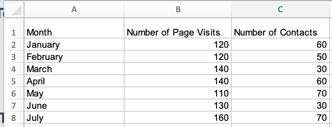
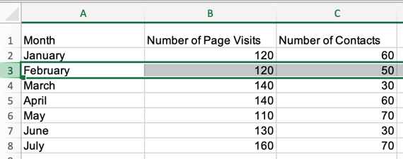
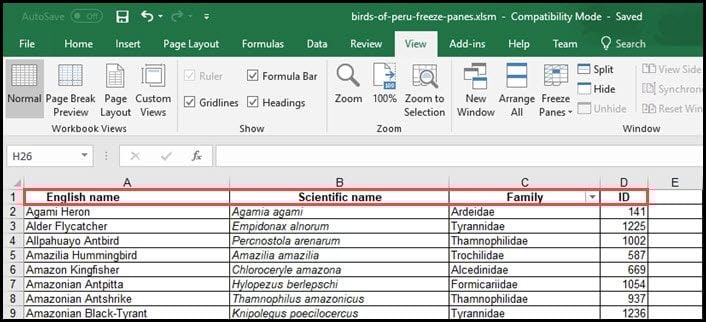
The image below is the sample data set I’ll use to run through the explanations in this piece.

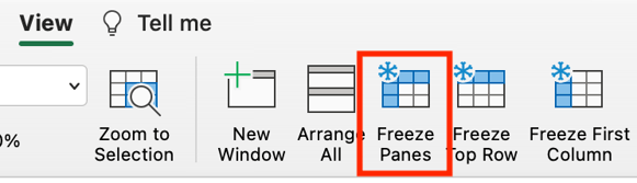
1. To freeze the top row in an Excel spreadsheet, navigate to the header toolbar and select View, as shown in the image below.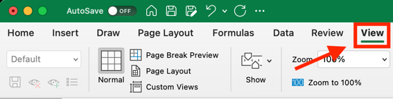

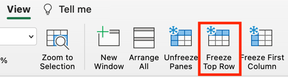
2. When the View menu options appear, Click Freeze Top Row, outlined in red in the image below.

Once selected, everything in the top row of your Excel spreadsheet (row 1) will be frozen, and you can scroll up and down in your spreadsheet, but the top rows won’t move, as shown in the gif below.

How to Freeze a Specific Row in Excel

While excel has native functions for freezing the top row of a data set and the first column of a data set, there are additional steps to take to freeze other elements of your data set that aren’t those two things.

1. To freeze a specific row in Excel, select the row number immediately underneath the one you want frozen. For this example, I’m selecting row number three to freeze row number two.

2. After selecting your row, navigate to View in the header toolbar and select Freeze Panes.

Once selected, you’ll be able to scroll up and down through your spreadsheet and always see row two.

Note that using the Freeze Panes function to freeze rows also freezes every row above the row you initially selected. For example, in the gif below, I selected row five which also freeze rows four, three, two, and one.

How to Freeze the First Column in Excel

1. To freeze the first column of your Excel spreadsheet (column A), navigate to the Excel header toolbar, select View, and click Freeze First Column.

Once selected, you’ll be able to scroll side to side within your sheet, and the first column of your data set will always be visible, as shown in the image below.

How to Freeze a Specific Column in Excel

1. If you want to freeze a specific column in excel, select the column letter that is immediately next to the column you want frozen and click Freeze Panes in the View header menu.

Once selected, you can scroll side to side through your entire data set and continue to see those columns. In the gif below, I’ve frozen columns A and B.

Using the freeze function in Excel makes your spreadsheets easier to understand, as you can ensure that critical rows and columns are always visible as you scroll through your data.

Источник

How to Freeze Cells in Excel? (with Examples)

Freezing cells in Excel means that when we move down to the data or move up the cells, it freezes the cells displayed on the window. To freeze cells in Excel, we must select those cells we want to freeze. Then, in the “View” tab in the windows section, click on “Freeze Panes” and again click on “Freeze Panes” from the drop-down list. As a result, this will freeze the selected cells. First, let us understand how to freeze rows and columns in Excel by a simple example.

You can download this Freeze Rows and Columns Excel Cell template here – Freeze Rows and Columns Excel Cell template

How to Freeze Cells in Excel? (with Examples)
- Example #1
- Example #2
- Use of Rows & Column Freezing in Excel Cell
- Things to Remember
- Recommended Articles

Example #1

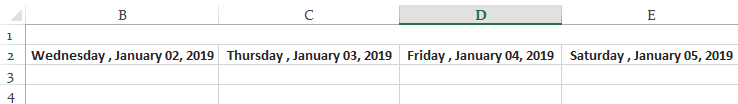
Freezing the Rows: Given below is a simple example of a calendar.

We must first select the row which we need to freeze the cell by clicking on the number of the row.
Then, click on the “View” tab on the ribbon. Next, we must select the “Freeze Panes” command on the “View” tab.
The selected rows get frozen in their position, and a grey line denotes it. We can scroll down the entire worksheet and continue viewing the frozen rows at the top. As we can see in the snapshot below, the rows above the grey line are frozen and do not move after we scroll the worksheet.
We can repeat the same process for unfreezing the cells. Once we have frozen the cells, the same command is changed in the “View” tab. The “Freeze Panes” in the Excel command is now changed to the “Unfreeze Panes” command. By clicking on it, the frozen cells are unfrozen. This command unlocks all the rows and columns to scroll through the worksheet.

The date is provided in the columns instead of the rows in this example.

Step 1: We need to select the columns, which we need to freeze Excel cells by clicking on the alphabet of the column.

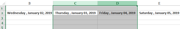
Step 2: After selecting the columns, we need to click on the “View” tab on the ribbon. Then, we need to choose the “Freeze Panes” command on the “View” tab.

Step 3: The selected columns get frozen in their position, and a grey line denotes it. We can scroll the entire worksheet and continue viewing the frozen columns. As we can see in the snapshot below, the columns beside the grey line are frozen and do not move after we scroll the worksheet.

For unfreezing the columns, we must use the same process as we did in the case of rows by using the “Unfreeze Panes” command from the “View” tab. In addition, there are two other commands in the “Freeze Panes” options: “Freeze Top Row” and “Freeze First Column.”

These commands are used only for freezing the top row and the first column, respectively. For example, the “Freeze Top Row” command freezes the row number “1,” and the “Freeze First Column” command freezes the column number A cell. It is to be noted that we can also freeze rows and columns together. In addition, It is not necessary to lock only the row or the column at a single instance.

Example #2

Let us take an example of the same.

Step 1: The sheet below shows the timesheet of a company. The columns contain the headers as “Day,” “Date,” “Regular Hours,” “Overtime Hours,” “Sick,” “Vacation,” and “Total.”

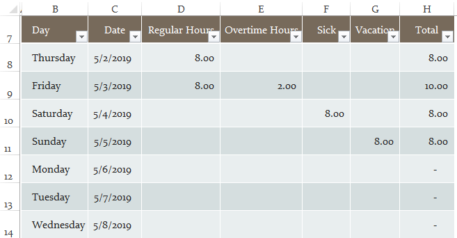
Step 2: We need to see columns “B” and row 7 throughout the worksheet. We have to select the cell above, besides which we need to freeze the columns and rows cells, respectively. In our example, we have to choose the cell number H4.

Step 3: After selecting the cell, we need to click on the “View” tab on the ribbon and select the “Freeze Panes” command on the “View” tab.

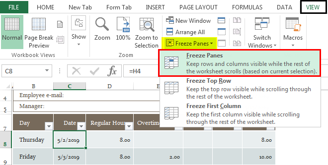
Step 4: As we can see from the snapshot below, two grey lines denote the locking of cells.

Use of Rows & Column Freezing in Excel Cell

If we use the “Freeze Panes” command to freeze the columns and rows of Excel cells, they will remain displayed on the screen regardless of the magnification settings that we select or how we scroll through the cells. Let us take a practical example of the weekly attendance report of a class.

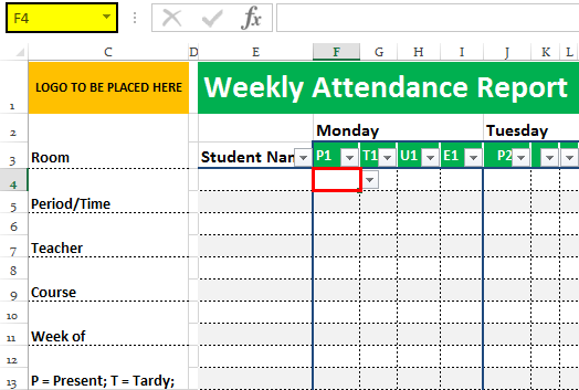
Step 1: Now, if we take a look at the snapshot below, the rows and columns display various pieces of information such as “Student name,” “Name of the days,” “Room,” etc. The topmost column shows the “logo to be placed here” and the “Weekly Attendance Report.”

In this case, it becomes necessary to freeze certain Excel columns and rows of cells to understand the attendance of the reports. Otherwise, the report becomes vague and difficult to understand.

Step 2: We must select the cell at the F4 location as we need to freeze down the rows up to the subject code P1, T1, U1, E1, and columns up to the “Student Name.”

Step 3: Once we select the cell, we must use the “Freeze Panes” command, freezing the cells at the position indicating a grey line.

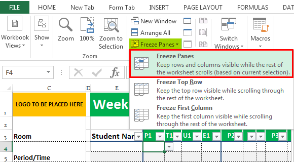
As a result, we can see that the rows and columns beside and above the selected cell have been frozen, as shown in the snapshots below.

Similarly, we can use the “Unfreeze Panes” command from the “View” tab to unlock the cells which we have frozen.

Hence, explaining the examples above, we used the freezing of rows and columns in Excel.

Things to Remember

When we press the “Ctrl+Home” Excel Shortcut keysAn Excel shortcut is a technique of performing a manual task in a quicker way.read more after giving the “Frozen Panes” command in a worksheet, instead of positioning the cell cursor in cell A1 as normal, Excel sets the cell cursor in the first unfrozen cell.
The “Freeze Panes” in the worksheet cell display consist of a feature for printing a spreadsheet known as “Print Titles.” When we use Print TitlesIn Excel, Print Titles is a feature that lets the users print specific row & column headings on every page of a multi-page report. You need to select “Print Titles” in the Page Layout Tab & enter the required details to perform the function. read more in a report, the columns and rows that we define as the titles are printed at the top and to the left of all data on each report page.
The shortcut keys that get random access to the “Freezing Panes” command are “Alt+W+F.”
In the case of freezing Excel rows and columns together, we must select the cell above, and the rows and columns need to be frozen. We do not have to select the entire row and column together for locking.

Here we have 3 easy steps that help you understand how to freeze cells in excel.

It keeps the row visible while you scroll through the rest of the sheet. It is very useful when working with a lot of data. Excel now allows more than a million rows and over 15,000 columns so, needless to say, workbooks can become extremely large and difficult to navigate.

The ability to freeze rows in excel will prevent having to scroll up and down repeatedly to view the column titles of the data or similarly to freeze columns in excel will prevent the constant sliding back and forth horizontally.

Under the VIEW tab on the top menu bar, you may select FREEZE PANES and you will see three options for freezing sections of data.

Freeze Panes excel is the first option. This allows you to keep several rows frozen while you navigate through the rest of the data. It is highly useful when there are more categories or subcategories in the header rows.

How To Freeze a Row In Excel: A Simple Example

This type of data would have “Address” in Row 1 merged across several cells and Row 2 would have “Street Address”, “City”, “State”, etc. underneath the “Address” Category. You could freeze both Row 1 and 2 to keep all headers visible.

How To Do This?

Select the Row under the rows you would like to freeze by clicking on the row number to the left of each row. For the Address example, we would click on Row 3 because we want to view Rows 1 and 2.
Under the VIEW tab select FREEZE PANES.
Select FREEZE PANES again. A grey line will appear to show what rows will be frozen in place.

The Second Option

For freezing rows of data, you have to Freeze the First Row. This will freeze only the first row of the workbook to keep it visible as you scroll through the data. It is most useful when the data has just one header in the top row. You do not need to select the first row to freeze top row excel because you simply need to follow step 2 given above and select FREEZE TOP ROW Excel.

If at any time, you wish to unfreeze the rows you return to the VIEW tab and select UNFREEZE ROWS. The grey line will disappear and frozen rows will no longer stay visible as you scroll vertically through the workbook.

How to Freeze Columns in Excel?

Columns May Also Be Frozen By Following The Same Steps

As above but choosing the column instead of the row and selecting FREEZE PANE which will allow you to scroll Horizontally through the workbook and keep the columns to the left of the grey indicator line frozen in place. The third option is to FREEZE the FIRST COLUMN, which is exactly like freezing the first row.

Be cautious when locking several rows at once as some may become hidden and you won’t be able to see those cells later as you are scrolling. To resolve this issue, make absolutely sure that any rows you are attempting to lock are visible when you select the FREEZE PANES option.

Other view options that Excel offers are opening a new window to view your workbook or splitting the workbook to view several sections at a time.

Источник

When you’re working with a lot of spreadsheet data on your laptop, keeping track of everything can be difficult. It’s one thing to compare one or two rows of information when dealing with a small subset of data, but when a dozen rows are involved, things get unwieldy. And we haven’t even started talking about columns yet. When your spreadsheets become unmanageable, there’s only one solution: freeze the rows and columns.

Freezing rows and columns in Excel makes navigating your spreadsheet much easier. When done correctly, the chosen panes are locked in place; this means those specific rows are always visible, no matter how far you scroll down. More often than not, you’ll only freeze a couple of rows or a column, but Excel doesn’t limit how many of either you can freeze, which can come in handy for larger sheets.

This how-to works with Microsoft Excel 2016 as well as later versions. However, the this method also works with Google Sheets, OpenOffice and LibreOffice. Ready to get to work? Here’s how to freeze rows and columns in Excel:

More: How to put Windows 10 into Safe Mode
Here’s how to lock cells in Excel and how to recover a deleted or unsaved file in Excel
This is how to use VLOOKUP in Excel and add additional rows above or below in Excel

How to freeze a row in Excel

1. Select the row right below the row or rows you want to freeze. If you want to freeze columns, select the cell immediately to the right of the column you want to freeze. In this example, we want to freeze rows 1 to 5, so we’ve selected row 6.

(Image credit: Future)

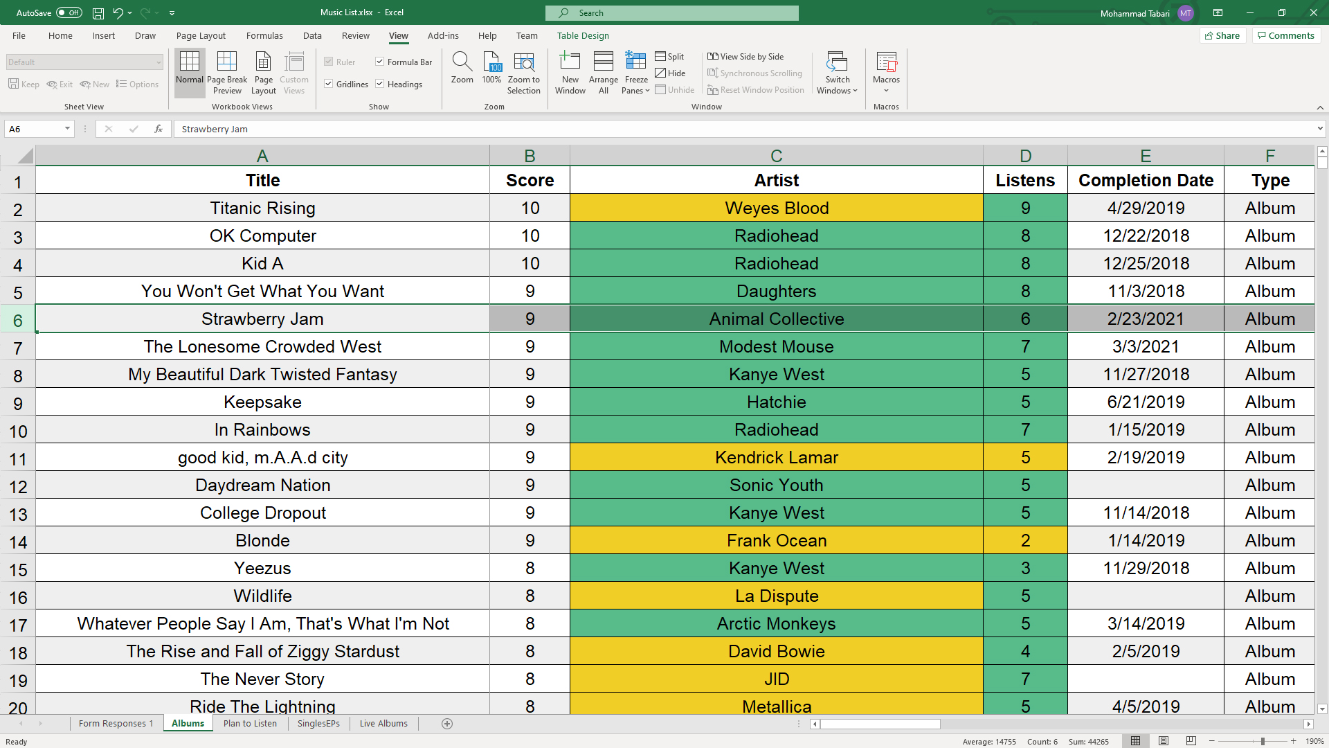
2. Go to the View tab. This is located at the very top, inbetween «Review» and «Add-ins.»

3. Select the Freeze Panes option and click «Freeze Panes.» This selection can be found in the same place where «New Window» and «Arrange All» are located.

(Image credit: Future)

That’s all there is to it. As you can see in our example, the frozen rows will stay visible when you scroll down. You can tell where the rows were frozen by the green line dividing the frozen rows and the rows below them.

(Image credit: Future)

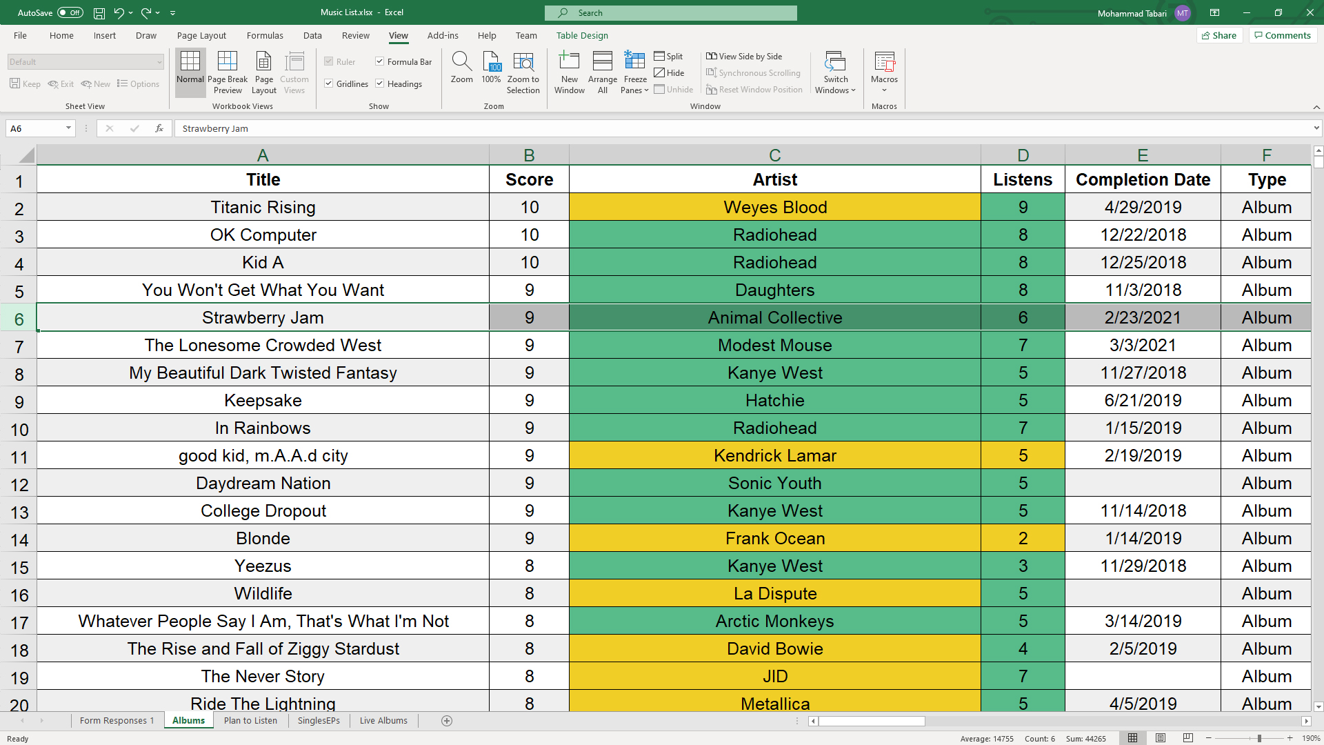
If you want to unfreeze the rows, go back to the Freeze Panes command and choose «Unfreeze Panes».

(Image credit: Future)

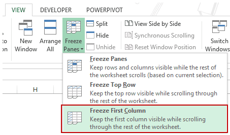
Note that under the Freeze Panes command, you can also choose «Freeze Top Row,» which will freeze the top row that’s visible (and any others above it) or «Freeze First Column,» which will keep the leftmost column visible when you scroll horizontally.

Besides allowing you to compare different rows in a long spreadsheet, the freeze panes feature lets you keep important information, such as table headings, always in view.

Need more Excel tricks? Check out our tutorials on How to Lock Cells in Excel and How to Use VLOOKUP in Excel.

Get instant access to breaking news, the hottest reviews, great deals and helpful tips.

Источник

Watch Video – Using Excel Freeze Panes

When working with large data sets, if you scroll down or to the right of the worksheet you would lose track of the row/column headings.

In such situations, you can use the Excel Freeze Panes feature to freeze the rows or columns in your dataset – so that the headers always visible no matter where you scroll in your data.

Accessing Excel Freeze Panes Options

To access Excel Freeze Panes options:

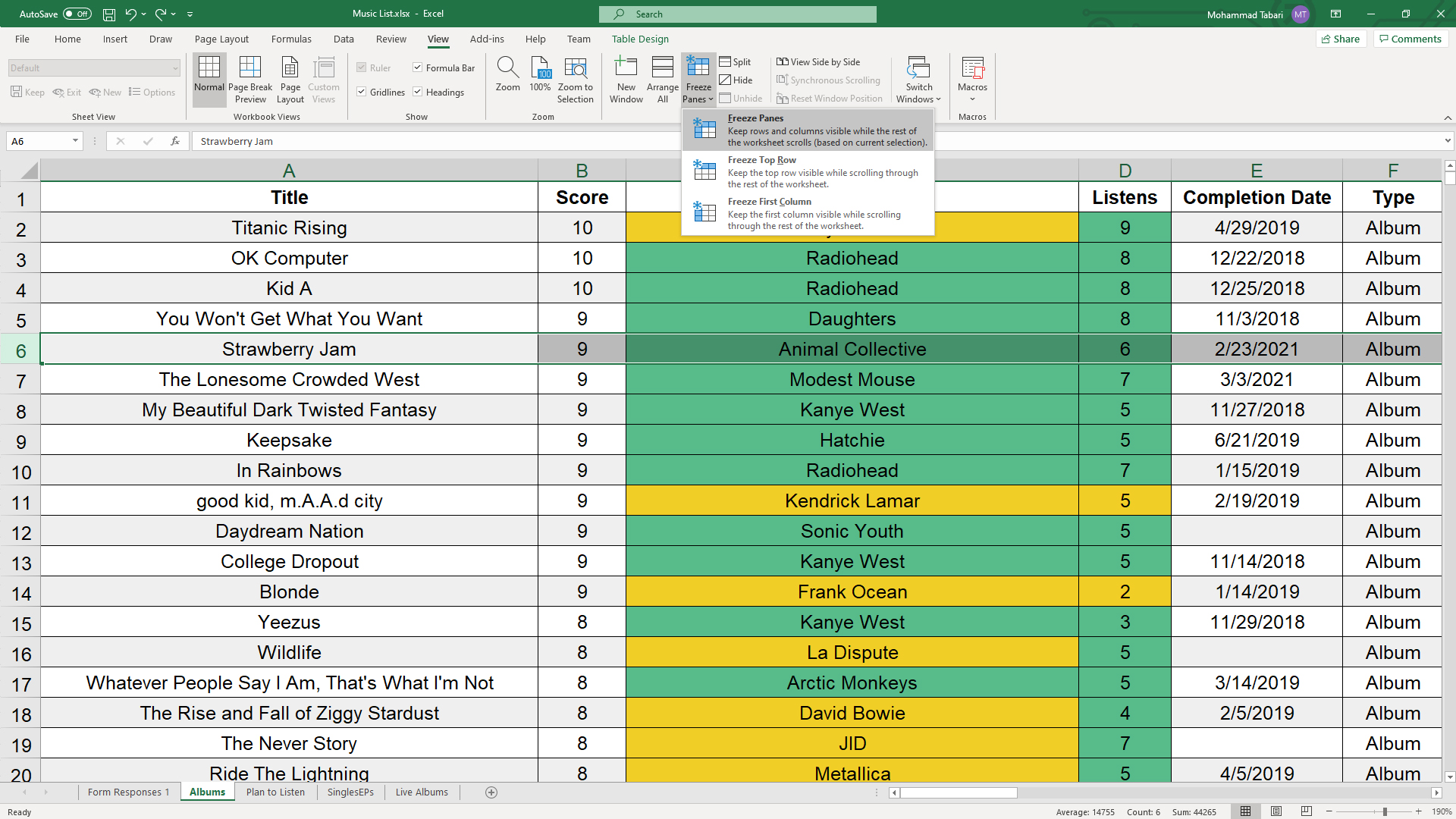
It shows three options in the Freeze Panes drop-down:

Freeze Panes: It freezes the rows as well as the columns.
Freeze Top Row: It freezes all the rows above the active cell.
Freeze First Column: It freezes all the columns to the left of the active cell.

You can use these options to lock rows or columns (or both) into panes in Excel.

Let’s see how to use these options to Freeze Panes in Excel while working with large data sets:

Freezing Row(s) in Excel

If you are working with a dataset that has headers at the top row and a dataset that spans hundreds of rows, as soon as you scroll down, the headers/labels would disappear.

Something as shown below:

In such cases, it’s a good idea to freeze the header row so that these are always visible to the user.

In this section, you’ll learn how to:

How to Freeze the top row.
How to Freeze more than one row.
How to Unfreeze rows.

Freeze the Top Row in Excel

Here are the steps to freeze the first row in your dataset:

Now when you scroll down, the row that has been frozen would always be visible. Something as shown below:

Freeze/Lock More than One Row in Excel

If you have more than one header rows in your dataset, you may want to freeze all of it.

Here is how to freeze rows in Excel:

Select the left-most cell in the row which is just below the headers row.
Click the ‘View’ tab.
In the Zoom category, click on the Freeze panes drop down

In the Freeze Panes drop-down, select Freeze Panes.
This will freeze all the rows above the selected cell. You would notice that a gray line now appears right below the rows that have been freezed.

Now when you scroll down, all the header rows would always be visible. Something as shown below:

Also read: How to Freeze Multiple Columns in Excel?

Unfreeze Rows in Excel

To unfreeze row(s):

Excel Freeze Panes Options – Freezing Column(s)

If you are working with a dataset that has headers/labels in a column and the data is spread across many columns, as soon as you scroll to the right, the header would disappear.

Something as shown below:

In such cases, it’s a good idea to freeze the left-most column so that the headers are always visible to the user.

In this section, you’ll learn how to:

How to Freeze the Left-most Column.
How to Freeze more than one Column.
How to Unfreeze Columns.

Freeze/Lock the Left-Most Column in Excel

Here is how to freeze the left-most column:

Now when you scroll down, the left-most column would always be visible. Something as shown below:

Additional Notes:

Once you freeze a column, you can not use Control + Z to unfreeze it. You need to use the unfreeze option in the Freeze Panes drop-down.
If you insert a column to the left of the column that has been frozen, even the inserted column is frozen.

Freeze/Lock More than One Column in Excel

If you have more than one column that contains headers/labels, you may want to freeze all of it.

Here is how to do this:

Select the top-most cell in the column which is right next to the columns that contain headers.
Click the ‘View’ tab.
In the Zoom category, click on the Freeze panes drop-down

In the Freeze Panes drop-down, select Freeze First Column.
This will freeze all the columns to the left of the selected cell. You would notice that a gray line appears to the right of the columns that have been frozen.

Now when you scroll to the right, all the columns with headers would always be visible. Something as shown below:

Unfreeze Columns in Excel

To unfreeze column(s):

Freezing Both Row(s) & Column(s)

In most of the cases, you would have the headers/labels in rows as well as in columns. In such cases, it makes sense to freeze both rows and columns.

Here is how you can do this:

Now when you scroll down or to the right, the frozen rows and columns would always be visible. Something as shown below:

You can unfreeze the frozen rows and columns at one go. Here are the steps:

Notes:

Apart from working with large data sets, one practical use where you may want to freeze panes in Excel is when you are creating dashboards. You can freeze rows and columns that contain the dashboard so that the user can’t scroll away and the dashboard is always visible.
A good practice while working with large data sets is to convert it into Excel Tables. By default, all the row headers in Excel Tables are always visible when you scroll within the dataset.

You May Also Like the Following Excel Tutorials:

Excel Data Entry Tips
How to Lock Cells in Excel.
How to Lock Formulas in Excel.
Compare Columns in Excel
Move Rows and Columns in Excel
Delete Blank Rows in Excel
Highlight Rows Based on a Cell Value in Excel
How to Turn OFF Scroll Lock in Excel?

Источник

I recently helped a friend with Excel, and when I asked him how the spreadsheet looked, he hesitated. Finally, he looked at me and said, “It’s overwhelming.” The data was OK, but he wanted to see the top row when he scrolled. The solution was to show him how to freeze rows and columns in Excel so that key headings or cells were always visible. I’ve outlined four scenarios and solution steps.

This was a good communication lesson for me. It reminded me that we all have different skill levels and vocabularies. For example, when you’re new, you’re probably not thinking in terms like “how to freeze panes in Excel.” You may not know what a pane is. It’s not describing your problem. My friend was thinking in terms of a “sticky header,” or “Excel floating header,” or “pinning rows.” I wasn’t thinking of any of those.

Let’s Start with Excel Panes

An Excel pane is a set of columns and rows defined by cells. You get to determine the size, shape, and location. For many people, it might be the top row. For others, it’s an inverted L-shape and contains the top row and first column. You’re the spreadsheet architect and can define your pane.

Regarding spreadsheets, you can “freeze panes” or “split panes.” Splitting panes is a bit more complex because you have separate windows of your data on the worksheet. So, for the sake of simplicity, this tutorial will cover freezing panes.

If your columns and rows aren’t in the orientation you want, you may want to learn how to transpose or switch columns and rows in Excel.

Why Lock Spreadsheet Cells?

A key benefit to locking or freezing cells is seeing the important information regardless of scrolling. The split pane data stays fixed. Your spreadsheet can contain panes with column headings, multiple rows, multiple columns, or both.

Otherwise, losing focus on a large worksheet is easy when you don’t have column headings or identifiers. I’ve had times where I’ve entered data only to see I was one cell off and produced Excel formula errors. By locking various sections, you have a consistent reference point. This also helps readability.

Typically, the cells you want to stay sticky are labels like headers. However, they could just as easily be an entire column, such as employee names.

Let’s go through four examples and keyboard shortcuts to freeze panes in Excel.

1 – How to Freeze the Top Row

This freeze row example is perhaps the most common because people like to lock the top row that contains headers, such as in the example below.

Another solution is to format the spreadsheet as an Excel table.

Locking the Top Row with Headings

Open your worksheet.
Click the View tab on the ribbon.
On the Freeze Panes button, click the small triangle ▼ (drop-down arrow) in the lower right corner. You should see a new menu with three options.

The Main Freeze Panes Options

Click the menu option Freeze Top Row.
Scroll down your sheet to ensure the first row stays locked at the top.

You should see a darker border under row 1.

Keyboard Shortcut – Lock Top Row

I like to do this shortcut slowly the first time to see the ALT key letter assignments as you type. I can see the keyboard assignments in the example below once I hit my Alt key. Some people prefer to add the Freeze Panes command to the Quick Access toolbar because they frequently use it.

Keyboard Shortcut Letters

Alt + w + f + r

2 – How to Freeze the First Column

A similar scenario is when you want to freeze the leftmost column. I guess Microsoft researched this to determine the most common sub-menu options.

I find this option helpful when I have a spreadsheet with many columns and I need to fill in data without using an Excel data form.

Freeze the first column of Excel

Open your Excel worksheet.
Click the View tab on the ribbon.
On the Freeze Panes button, click the small triangle ▼. You should see a new menu with your 3 options.
Click the option Freeze First Column.
Scroll across your sheet to make sure the left column stays fixed.

Keyboard Shortcut – Lock First Column

Alt + w + f + c

3 – How to Freeze the Top Row & First Column

Frozen pane area in red

This is my favorite option. If you look at Microsoft’s initial Freeze Panes options, there isn’t one for the top row and first column. Instead, we’ll use the generic option called Freeze Panes.

The subtext reads, “Keep rows and columns visible while the rest of the worksheet scrolls (based on current selection).” Some folks get confused as they think they have to highlight data to make a selection.

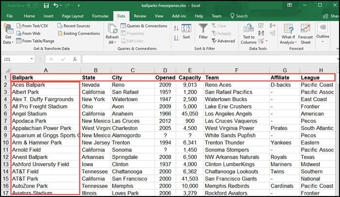
Instead, consider the selection of the first cell outside your fixed column and row. If I wanted to lock the top row and top column, that selection cell would be cell B2 or Nevada. Regardless of whether I scroll down or to the right, the first cell that disappears when I scroll is B2.

The Freeze Pane Selection Cell is in green.

Open your Excel spreadsheet.
Click cell B2. (Your set cell.)
Click the View tab on the ribbon.
On the Freeze Panes button, click the small triangle ▼ in the lower right corner. You should see a dropdown menu with your 3 options.
Click the option Freeze Panes.
Scroll down your worksheet to make sure the first row stays at the top.
Scroll across your sheet to make sure your first column stays locked on the left.

Keyboard Shortcut – Freeze Panes

Alt + w + f + f

4 – Freeze Multiple Columns or Rows

On occasion, I get some Excel worksheets where the author puts descriptive text above the data. My header isn’t in Row 1 but further down in Row 5. Or I want to lock multiple columns to the left. In the example below, I want to lock Columns A & B and Rows 1-5.

Frozen columns A&B; Frozen rows 1-5

The process is the same, I just need to click the set cell that stops the fixed area. In this case, it would be cell C6 or “Regions Field.” The content above and to the left is frozen.

Everything in the red boxes would be locked. The downside is you may give up much of the screen real estate.

Why Freeze Panes May Not Work

There are some rules surrounding this feature. If you don’t follow these, freeze panes may not work.

Quick test: If you type Ctrl + Home and your cursor moves to cell A1, you haven’t locked anything.

If you dislike your settings, use the Unfreeze Panes command.
This feature won’t work on a protected worksheet or Page Layout View.
If you’re editing a value in the Formula bar, the View menu will be disabled.

If you need to see the same header on printed pages, Microsoft has instructions.

As you’ve seen, choosing what content to freeze is easy. You can freeze the top row, first column, both, or a subset of your data, depending on what you want to do with it. The flexibility is part of what makes Microsoft Excel such an excellent program for organizing and analyzing information from any field.

Источник

Freeze rows or columns

Unfreeze rows or columns

Need more help?

See Also

Need more help?

Want more options?

Freeze First Row

Freeze First Column

Freeze Panes

Freeze Panes – Multiple Rows

Freeze Panes – Multiple Columns

Freeze Panes – Multiple Rows and Columns both

Unfreeze Panes:

Freeze panes versus Splitting Panes:

Is Freeze Pane option disabled?

How to Freeze a Top Row in Excel

How to Freeze a Specific Row in Excel

How to Freeze the First Column in Excel

How to Freeze a Specific Column in Excel

How to Freeze Cells in Excel? (with Examples)

Table of contents

Example #1

Example #2

Use of Rows & Column Freezing in Excel Cell

Things to Remember

Recommended Articles

Here we have 3 easy steps that help you understand how to freeze cells in excel.

How To Freeze a Row In Excel: A Simple Example

The Second Option

How to Freeze Columns in Excel?

Columns May Also Be Frozen By Following The Same Steps

How to freeze a row in Excel

Accessing Excel Freeze Panes Options

Freezing Row(s) in Excel

Freeze the Top Row in Excel

Freeze/Lock More than One Row in Excel

Unfreeze Rows in Excel

Excel Freeze Panes Options – Freezing Column(s)

Freeze/Lock the Left-Most Column in Excel

Freeze/Lock More than One Column in Excel

Unfreeze Columns in Excel

Freezing Both Row(s) & Column(s)

Let’s Start with Excel Panes

Why Lock Spreadsheet Cells?

1 – How to Freeze the Top Row

Keyboard Shortcut – Lock Top Row

2 – How to Freeze the First Column

Keyboard Shortcut – Lock First Column

3 – How to Freeze the Top Row & First Column

Keyboard Shortcut – Freeze Panes

4 – Freeze Multiple Columns or Rows

Why Freeze Panes May Not Work